9

The Arc and Interruption

Paul G. Slade

All the elements of earth except Hydrogen and some Helium … were made in the interiors of collapsing stars. We are made of star stuff.

Cosmos, Carl Sagan

CONTENTS

9.1      Introduction

9.2      The Fourth State of Matter

9.3      Establishing an Arc

9.3.1      Long-Gap Gas Breakdown

9.3.2      Vacuum Breakdown and Short-Gap Breakdown

9.3.3      The Volt–Current Characteristics of Separated Contacts

9.4      The Formation of the Electric Arc

9.4.1      The Formation of the Electric Arc During Contact Closing

9.4.2      The Formation of the Electric Arc During Contact Opening

9.5      The Arc in Air at Atmospheric Pressure

9.5.1      The Arc Column

9.5.2      The Cathode Region

9.5.3      The Anode Region

9.5.4      The Minimum Arc Current and the Minimum Arc Voltage

9.5.5      Arc Volt–Ampere Characteristics

9.6      The Arc in Vacuum

9.6.1      The Diffuse Vacuum Arc

9.6.2      The Columnar Vacuum Arc

9.6.3      The Vacuum Arc in the Presence of a Transverse Magnetic Field

9.6.4      The Vacuum Arc in the Presence of an Axial Magnetic Field

9.7      Arc Interruption

9.7.1      Arc Interruption in Alternating Current Circuits

9.7.1.1      Stage 1 – Instantaneous Dielectric Recovery

9.7.1.2      Stage 2 – Decay of the Arc Plasma and Dielectric Reignition

9.7.1.3      Thermal Reignition

9.7.2      Arc Interruption in Direct Current Circuits

9.7.3      Vacuum Arc Interruption in Alternating Circuits

9.7.4      Arc interruption of Alternating Circuits: Current Limiting

9.7.5      Interruption of Low Frequency and High Frequency Power Circuits

9.7.6      Interruption of Megahertz and Gigahertz Electronic Circuits

Acknowledgments

References

9.1    Introduction

The first eight chapters of this book have discussed fixed contacts. You have explored the physical effects of two metals in contact and the effect of chemical reactions at the contact interface. By using these fundamental principles, you have been shown how it is possible to design fixed contacts for a very wide range of currents: e.g., from connectors for power circuits that pass many thousands of amperes and must survive short circuit currents of over 10⁵ A to connectors for electronic equipment that can see currents as low as 10⁻⁹ A. With this chapter, you will now begin to study the equally interesting effects that occur as you separate two contacts in order to interrupt the flow of current in a circuit. For the most part, I will be concerned with currents greater than 10 mA and circuit voltages greater than a few volts. The range of currents and voltages will be discussed in detail later in this chapter. This range of course covers a vast array of switching devices from small ac and dc relays and switches to large circuit breakers that interrupt high-power circuits.

This chapter concentrates upon the electric arc, its structure, how is it formed, and how it is used to interrupt electric current. Chapter 10 will discuss the general effect of arcing upon the electric contacts and Chapter 11, Chapter 12, Chapter 13, Chapter 14 Chapter 15 will show how these effects can be used to design a wide range of switching devices. Chapter 16, Chapter 17, Chapter 18 and Chapter 19 then will discuss the range of contact materials used for switching, their manufacture, their construction and attachment, how they are tested, and the chemical effects of contaminants.

9.2    The Fourth State of Matter

The ancient Greeks thought the world was composed form four states of matter: “earth,” “water,” “vapor,” and “fire.” Three thousand years later, we now believe the universe is still composed of four states of matter, but now they are: “solids,” “liquids,” “gases,” and “plasmas.” The first three states of matter are to be found only on cold planets such as the Earth and as meteoric matter. The fourth, the plasma state, is the predominant state of matter in the universe. The stars, the nebulae, the intergalactic gas, the solar winds and the earth’s upper atmosphere are all in the plasma state. The first three states of matter, however, are common to our daily experience and will serve as a starting point to develop some basic concepts related to the ideas of “states of matter.”

A solid object such as a copper rod, for example, has a shape. It can be squeezed, hammered, bent, etc., into a shape and will retain its shape if left undisturbed. A liquid has no shape. It is characterized by volume, i.e., a liquid flows and assumes the shape of the container that holds it. A gas has no shape or volume. A gas expands to fill the container that holds it and exerts a pressure on the walls of the container. As a solid is heated it melts to form a liquid, and when the liquid is heated it eventually forms a molecular gas. We know that temperature is associated with the average kinetic energy of the molecules, and that the kinetic energy of the molecules is associated with their average velocity. The shape of the solid is defined by long-range intermolecular forces which overcome the kinetic energy of the molecules. As the kinetic energy of the molecules is increased by adding heat the intermolecular forces still hold the molecules together, but when the thermal energy is greater than the energy needed to hold collective groups of molecules in a shape, a liquid is formed. As more heat is added the average kinetic energy exceeds any intermolecular binding energy, and all molecules act independently, and the liquid becomes a molecular gas. As still more heat is added the gas molecules bounce off the walls of the container in which they are contained. They also collide with each other. It is now important to have some knowledge of the kinetic theory of gases. This is a very well-developed subject and if you are unfamiliar with this subject, I would recommend that you consult one of the many excellent books on the subject [1,2]. Here, only a very brief summary is given.

The molecules or atoms of a gas are in random motion and are colliding frequently with each other and the walls of the vessel in which they are contained. These collisions are elastic, i.e., energy and momentum are conserved and they have no preferred direction, all directions being equally probable. The collisions cause a continual interchange of energy. This energy has a steady-state distribution which can be derived using statistical techniques [2]. It can be shown that the overall kinetic energy of the gas and the average kinetic energy of each atom depend upon the absolute temperature T. The kinetic energy is divided equally between the degrees of freedom, each degree of freedom having $\left(1/2\right)kT$, where k is Boltzmann’s constant (1.38 × 10⁻²³ J K⁻¹). Thus for a monatomic gas with three degrees of freedom:

$\frac{1}{2}m\overline{c^2}=\frac{3}{2}kT$

(9.1)

where m is the mass of the gas atom, $\overline{c^2}$ is the mean square speed. Thus the total kinetic energy per cubic meter of a monatomic gas is

$\text{Total}\text{kinetic}\text{energy}=\frac{3}{2}nkT$

(9.2)

where n is the number of gas atoms per cubic meter. For a diatomic gas such as N₂, which has two more degrees of freedom, rotational and vibrational, the total kinetic energy is (5/2)nkT. It follows from Equation 9.1 that the mean square speed for a monatomic gas is given by 3kT/m. A useful parameter is the mean speed $\overline{c}$, which has a similar value to the square root of $\overline{c^2}$, but is not equal to it (since “mean” and “root mean square; RMS” are defined differently)

$\overline{c}={\left(\frac{8kT}{\text{π}m}\right)}^{1/2}$

(9.3)

By using the term mean speed $\overline{c}$ we are assuming that some atoms travel slower than $\overline{c}$ and others faster. By considering the random nature of these collision processes, Maxwell and Boltzmann showed that the number dn of atoms out of a total n that have speed between c and c + dc is given by (2):

$\frac{\text{d}n}{\text{d}c}=\frac{4n}{{\text{π}}^{1/2}}{\left(\frac{m}{2kT}\right)}^{3/2}{c}^{2}exp\left(-\frac{m{c}^2}{2kT}\right)$

(9.4)

The Maxwell–Boltzmann distribution function is shown in Figure 9.1. As can be seen, while some atoms travel very much faster and others very much slower than mean velocity $\overline{c}$, nearly 90% of them have speeds between $\left(1/2\right)\overline{c}$ and $2\overline{c}$ at any given time. The most probable speed is $c_0={\left(2kT/m\right)}^{1/2}$. The pressure p of the gas is given by

$p=\frac{nm\overline{c^2}}{3}\text{or}nkT$

(9.5)

If the gas is molecular, and still more heat is added, the average kinetic energy of the molecules will exceed the binding energy of the molecules and the molecules will dissociate into individual atoms. Upon further heating the atoms will be ionized, i.e., they will start to lose an electron. This will leave the normally neutral atoms with a positive charge; we call an atom in this state a positive ion (or, in most cases in this text, an ion for short). The mixture of ions and electrons is called the fourth state of matter or “plasma state.” A plasma can be defined as:

Any system in which there are free electrons and ions where the spatial and temporal average density of charges of each sign are approximately equal.

In the context of electric contacts, the plasma is ionized gas that ‘burns’ between parted contacts and is called an electric arc, or arc for short. The equality of the charge densities (i.e. quasineutrality) is an extremely important property and it will be used later in this chapter when discussing the current interruption process using the electric arc.

The term “arc” was first introduced by Sir Humphrey Davy [3] in the early 19th century, who, observing a discharge between two horizontal conductors, saw the hot luminous portion in the middle rise by convection while the ends remained fixed. The term plasma was introduced over 100 years later by I. Langmuir to give the matter inside the arc a name. A qualitative understanding of a plasma and of an arc in particular had to wait until the discovery of the electron by Thompson in 1897 [4] and the Bohr model of the atom in 1901 [5]. The subject finally built a solid foundation with the publication of Townsend’s seminal work, “Electricity in Gases” in 1915 [6]. Since that time, many books have been written describing arcs, e.g., References [7,8,9,10,11], and on the more practical aspects of the use of arcs to interrupt electric circuits, e.g., References [12,13,14,15,16,17]. Unfortunately, only Holm’s book [14] and Browne’s book [17] are still in print. It is, therefore, my purpose in this chapter to give you a general understanding of the arc as it applies to electric contacts without exploring the detailed physics, which can be found elsewhere. My discussion will, of course, be based upon the vast body of research that has already been done and I will provide detailed references for those of you who wish to study this subject further.

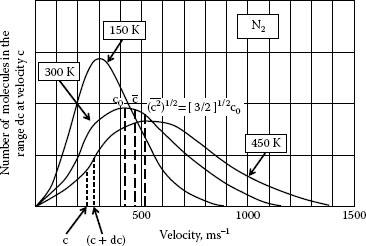
FIGURE 9.1
Example of Maxwell-Boltzmann speed distribution for nitrogen at three temperatures [17].

Without asking for the moment how we would do it, suppose we heat dry, atmospheric air to 25,000 K. With the help of Figure 9.2, we will follow what happens to the nitrogen and oxygen molecules as the temperature increases. At about 1,500 K the oxygen molecules begin to form monatomic oxygen atoms and for nitrogen molecule nitrogen molecules begin to dissociate and forms monatomic nitrogen atoms at about 2,500 K. At about 6,500 K both the oxygen and nitrogen atoms start to ionize and a plasma begins to form. By about 20,000 K there is almost no neutral gas left and the plasma is said to be fully ionized. As the temperature increases further, the oxygen and nitrogen ions gradually lose another electron and becomes doubly ionized. To strip all the electrons from these atoms, however, would require a plasma temperature of millions of degrees. For arcs that occur between electric contacts in switching devices, the temperature range is between approximately 6.0 K and approximately 20,000 K depending upon the arc current and other factors resulting from the design of the switch. At first sight, these temperatures seem very forbidding. Let us, for the moment, explore this aspect of the arc.

We know from Equation 9.1 that the kinetic energy of a gas is related to the absolute temperature T. Therefore, for a nitrogen ion (m = 2.3 × 10 ⁻²⁶ kg) at 20,000 K its root mean square velocity is

${\left(\overline{c^2}\right)}^{1/2}=4.9\times {10}^3{\text{ms}}^{-1}$

(9.6)

This seems to be a formidable velocity but it is easily achievable in the laboratory. If, for example, we take the glass tube shown in Figure 9.3, evacuate the gas from it, place a potential U across the electrodes and introduce a nitrogen ion at the positive electrode (the anode) it is possible to calculate the value of the potential drop U required to accelerate the ion to a velocity of 4.9 × 10³ ms⁻¹ by the time it reaches the negative electrode (the cathode). Kinetic energy of the ion at the negative electrode = potential energy of the ion at the positive electrode, that is,

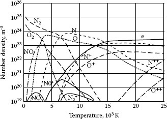
FIGURE 9.2
The number of particles per m³ for dry air at atmospheric pressure as a function of temperature.

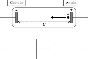
FIGURE 9.3
The acceleration of a nitrogen ion in vacuum.

$\frac{1}{2}m\overline{c^2}=\text{e}U$

(9.7)

where e is the charge which is 1.6 × 10⁻¹⁹ coulombs for an electron or for a singly ionized atom. Then for the nitrogen ion

$\frac{1}{2}\times 2.3\times {10}^{-26}\times 24.0\times {10}^6=U\times 1.6\times {10}^{-19}$

that is,

$U=1.7\text{V}$

(9.8)

So, using electrodes with a very low voltage across them, it is possible to accelerate an ion to a very high velocity, indeed a velocity that gives a very high equivalent temperature. This can only occur, however, if the tube is under high vacuum, where the nitrogen ion has a very low probability of colliding with another gas molecule. As soon as we introduce gas to the tube the elastic collisions between the ion and the gas quickly reduce the velocity of the ion to be in equilibrium with the background gas. We know from our experience with switching devices that they mostly operate in air at atmospheric pressure. How then does the gas between the contacts become ionized and an arc formed? The answer is to be found by considering the passage of the electrons through the gas.

9.3    Establishing an Arc

9.3.1    Long-Gap Gas Breakdown

Let us consider Figure 9.4, which illustrates possible interactions of an electron with gas molecules and atoms located between open contacts which have a constant voltage U impressed across them and are a distance d apart in air at atmospheric pressure. The voltage per unit distance i.e., U/d, is called the electric field E. If an electron is introduced into the gas between the contacts, being negatively charged, it drifts towards the anode and gains energy before it collides with a gas molecule or a gas atom. The energy an electron gains by travelling through a one volt drop in potential is 1 eV (1.6 × 10 ⁻¹⁹ J). The maximum energy the electron gains between collisions is:

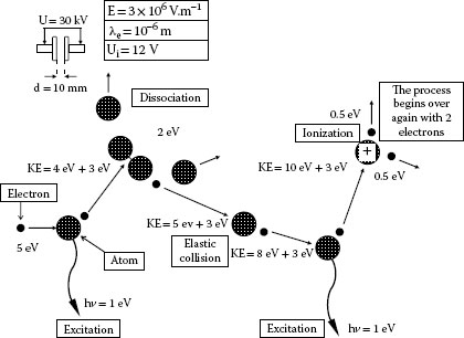
FIGURE 9.4
Possible interactions with a gas of an electron accelerated by an electric field.

$E{\text{λ}}_{\text{e}}=\frac{U{\text{λ}}_{\text{e}}}{d}$

(9.9)

where λ_e is the average distance travelled by the electrons between collisions, and is called the electron mean free path. In the simplified example shown in Figure 9.4, the average energy gained by the electron between collisions with the gas is 3 eV (i.e. 3 × 10⁶ × 10⁻⁶ eV). The electron collides with the gas in two ways. The first is called an elastic collision [1,18]. Here the electron bounces off the gas molecule in the same way a small glass marble would off a large bowling ball. The collision preserves momentum and, because the electron mass m_e is much less than the gas’s mass, the electron energy loss is close to zero. After the collision, the electron continues to pick up energy from the electric field.

The second type of collision is called an inelastic collision. Here the electron transfers some of it energy to the gas atom or molecule. It is these collision processes that eventually lead to the formation of an electric arc. There are many types of inelastic collisions [18]. I shall only briefly describe three of them.

1.  Dissociation is the process of splitting a molecule. For example, a nitrogen molecule can be dissociated into two nitrogen atoms. Dissociation is possible if the electron energy is greater than the bond strength of the molecule.

$e+N_2\to e+N+N$

(9.10)

2.  Excitation and relaxation is the process by which light is emitted from the gas. Figure–9.5 illustrates the process. The impacting electron forces an electron in the atom to a higher energy level, leaving the atom in an excited state. The excited state is usually very unstable and the excited electron returns to its original energy state in less than a nanosecond. The energy difference between the states is given off as light.

$e+N\to N^{*}+e$

(9.11)

then

$N^{*}\to N+hv$

(9.12)

where h is Planck’s constant and v is the frequency of the light.

3.  Ionization is the process that directly results in an electric arc. If the impacting electron has an energy equal to or greater than the energy to remove the most weakly bound electron from the atom, then there is a chance that the impacting electron will remove this electron from the atom, see Figure 9.6. This process results in a positive ion and in two electrons; the original impacting electron and the electron freed from the atom.

$e+N\to 2e+N^{+}$

(9.13)

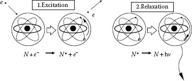
FIGURE 9.5
Excitation and relaxation produces radiation.

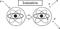
FIGURE 9.6
Ionization releases an electron from the atom leaving a positive ion.

The minimum energy to remove the weakest bound electron is called the ionization energy. Values of ionization potentials, V_i, for atoms useful for electric contacts, are given in Table 9.1. The energy an electron receives depends upon the strength of the electric field E and upon the distance it is accelerated between collisions. In Figure 9.4 there are three collisions before an atom is ionized (there may well be many more). When this occurs, two electrons are now free to interact with the gas. It only takes about 30 such doublings to produce 10⁹ electrons: this is termed a Townsend avalanche. The number of new ions produced per meter of path by the accelerated electron is inversely proportional to its mean free path λ_e. If α is the number of ionizing collisions per meter in the direction of the field, then:

TABLE 9.1
Values of Ionization Potential

Gas	Ionization Potential (V)
Air	14
A	15.7
CO2	14.4
H	13.5
N	14.5
O	13.5
Ag	7.6
Al	6.0
Cu	7.7
Ni	7.6
Mo	7.2
Sn	7.3
Pd	8.3
Pt	9.0
W	8.0

$\text{α = }\frac{f\left(E{\text{λ}}_{\text{e}}\right)}{{\text{λ}}_{\text{e}}}$

(9.14)

now f(Eλ) can be represented by

$f\left(E{\text{λ}}_{\text{e}}\right)=\exp \left(-\frac{V_i^{\prime }}{E{\text{λ}}_{\text{e}}}\right)$

(9.15)

where $V_i^{\prime }$ is an effective ionization potential

$\frac{1}{{\text{λ}}_{\text{e}}}=Ap$

(9.16)

where p is the gas pressure and A is a constant. Thus

$\text{α =}Apexp\left(-\frac{A{V}_i^{\prime }}{E/p}\right)$

(9.17)

α is called the first Townsend ionization coefficient [1,18]. Values for the mean free path of molecules (λ_g), ions (λ_i and electrons (λ_e) are given in Table 9.2.

If two contacts are separated by a distance d and if n₀ electrons per cubic meter are liberated from the cathode initially then the number n₁ of electrons per cubic meter arriving at the anode is

$n_1=n_{0}exp\left(\text{α}d\right)$

(9.18)

TABLE 9.2
Mean Free Path of Molecules, Electrons, and Ions at Atmospheric Pressure and Room Temperature

Gas	Molecular Mean Free Path, λg (nm)	Approximate Ion Free Path, ${\text{λ}}_{\text{i}}\approx \sqrt{}2{\text{λ}}_{\text{g}}$ (nm)	Approximate Electron Mean Free Path, ${\text{λ}}_{\text{e}}\approx 4\sqrt{}2{\text{λ}}_{\text{g}}$ (nm)
Air	96	135	180–545
A	99	140	295–560
CO2	61	86	185–345
H2	184	260	550–1,045
He	296	418	890–1,675
H2O	72.2	102	215–410
N2	93.2	132	280–530
Ne	193	273	580–1,095
N2O	70	99	210–395
O2	99.5	141	300–565
SO2	45.7	65	135–260

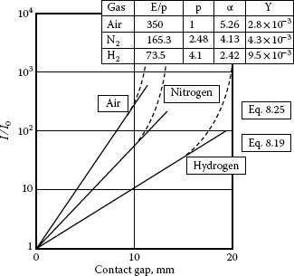
FIGURE 9.7
Typical log(I/I₀) versus contact gap curves for Townsend breakdown in air, nitrogen, and hydrogen [18].

or, converting this to current [18],

$I=I_{0}exp\left(\text{α}d\right)$

(9.19)

However as Figure 9.7 shows, if the ratio I/I₀ exceeds a given value, the increase in I exceeds the value calculated from Equation 9.19. As the current increases by the ionization process, the ions, ever increasing in number, drift toward the cathode. When these ions reach the cathode, they help liberate more electrons and thus increase I₀. The extra electrons liberated give rise to a secondary ionization process that causes the current to increase faster than in Equation 9.19. There have been other secondary processes formulated for the further liberation of electrons from the cathode such as photoelectric emission as well as enhanced ionization in the gas itself [18].

If we assume that the extra electrons are liberated by ion bombardment, then let us for a moment consider a number γ (called the second Townsend coefficient) of new electrons emitted from the cathode for each of the incoming positive ions. Again, let us also assume n₁ electrons per square meter reach the anode per second, that initially only n₀ electrons leave the cathode per square meter per second and that n_c is the total number of electrons per square meter per second that are liberated from the cathode from all the effects combined. The number of positive ions in the gas is equal to n₁ – n_c. The number of electrons leaving the cathode is

$n_c=n_0+\text{γ}\left(n_1-n_c\right)$

(9.20)

$n_c=\frac{n_0+\text{γ}{n}_1}{1+\text{γ}}$

(9.21)

Using Equation 9.18, the number of electrons reaching the anode is

$n_1=\frac{n_0+\text{γ}{n}_1}{1+\text{γ}}exp\left(\text{α}d\right)$

(9.22)

$n_1=\frac{n_{0}exp\left(\text{α}d\right)}{1-\text{γ}\left[exp\left(\text{α}d\right)-1\right]}$

(9.23)

or converting to current,

$I=\frac{I_{0}exp\left(\text{α}d\right)}{1-\text{γ}\left[exp\left(\text{α}d\right)-1\right]}$

(9.24)

Now

$exp\left(\text{α}d\right)>>1$

so:

$I=\frac{I_{0}exp\left(\text{α}d\right)}{1-\text{γ}exp\left(\text{α}d\right)}$

(9.25)

Thus as the electric field in the electrode gap increases, the current increases and there is a sudden transition from a “dark discharge” to one of a number of forms of sustained discharge. The initiation of a discharge based directly upon the mechanisms using the two Townsend coefficients is called Townsend breakdown. This transition, sometimes called a spark, consists of a sudden increase of current in the gap and is accompanied by a sudden increase in light visible between the contacts. It is this spark that initiates the arc. From Equation 9.25,

$I\to \infty as\text{γ}exp\left(\text{α}d\right)\to 1$

Let us assume the contact gap breaks down or sparks when

$In\frac{1}{\text{γ}}=\text{α}d$

(9.26)

When the gap d breaks down:

$E=\frac{V_{\text{B}}}{d}$

(9.27)

where V_B is the breakdown voltage or sparking potential. From Equation 9.17, we know that

$\text{α =}Apexp\left(-\frac{A{V}_i^{\prime }}{E/p}\right)$

(9.28)

Thus, at breakdown using, Equations 9.27 and 9.28,

$\text{α =}Apexp\left(-\frac{A{V}_i^{\prime }pd}{V_{\text{B}}}\right)$

(9.29)

Now, using Equation 9.26, and assuming breakdown occurs when I suddenly increases

$ln\frac{1}{\text{γ}}=Apdexp\left(-\frac{A{V}_i^{\prime }pd}{V_{\text{b}}}\right)$

(9.30)

$V_{\text{B}}=\frac{-A{V}_i^{\prime }pd}{ln\left(\frac{Apd}{ln\left[1/\text{γ}\right]}\right)}$

(9.31)

Thus the breakdown voltage V_B for a given gas with an effective ionization potential $V_i^{\prime }$ is a function of the gas pressure multiplied by the contact gap (pd) alone [11]. This is known as Paschen’s law, and was discovered in 1889 [19]. From Equation 9.5, $p=nkT$, so

$V_{\text{B}}=f\left(nd\right)$

(9.32)

Figure 9.8 shows a typical Paschen curves for air and SF₆ [20]. A qualitative explanation an easily be applied to it. For a given contact gap, at higher the pressures (to the right of the minimum value) the electron’s mean free path λ_e is smaller. The electrons, therefore, lose energy through more frequent collisions. In order to ensure a breakdown, the electric field must be high enough for the electrons to gain sufficient energy between collisions. As $E=V_{\text{B}}/d$ then V_B has to increase. At low values of pressure (to the left of the minimum value) the electron can now travel further before hitting an atom, but the probability of impact has decreased enough that each collision requires a higher probability for ionization. For this to occur, the electrons must gain more energy from the electric field and thus V_B has to increase again. Table 9.3 gives the minimum breakdown voltage (V_B)_min and minimum (pd)_min values for various gases. Note, that for a limited range of V_B there are two values of pd. Thus for a given V_B and gas pressure there are two possible electrode gaps at which breakdown can occur. Under some circumstances, therefore, the intuitive answer to an unwanted breakdown of increasing the contact gap and thus increasing the breakdown distance will not always apply.

In most careful experiments for measuring α and γ the initiating current I₀ is by photo emission or thermionic emission from the cathode. In most electric contact applications the initial electron current results from electrons that are liberated from the cathode by field emission (see Section 9.3.2) or by other random physical processes. There may well be a period of time when V_B across an open contact is exceeded (see Section 9.4.1), before breakdown begins, but once it is initiated, it can occur extremely quickly, see for example Figure 9.9.

FIGURE 9.8
Paschen curves for air and SF₆.

TABLE 9.3
Minimum Breakdown Voltage (V_B)_min and (pd)_min Values for Various Gases

Gas	(VB)min (V)	${\left(pd\right)}_{\text{min}}$ (10−3 torr, m)	dmin, cm (p = 1 atmosphere i.e., 760 torr)
Air	327	5.7	0.75 × 10−3
A	137	3.9	1.18 × 10−3
N2	251	6.7	0.83 × 10−3
H2	273	1.5	1.51 × 10−3
O2	450	7.0	0.92 × 10−3

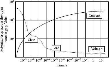
FIGURE 9.9
Time for contact gap breakdown and arc formation for a 1 mm contact gap.

9.3.2    Vacuum Breakdown and Short-Gap Breakdown

It is possible to apply a high enough voltage across open contacts in vacuum to cause breakdown. This is called vacuum breakdown. In spite of the name it is a breakdown process that occurs in metal vapor liberated from the contacts themselves. A detailed discussion of the processes that lead to vacuum breakdown can be found in References [20,21].

The process begins with electrons liberated from the cathode. Electrons can be removed from a metal by (1) providing them with sufficient kinetic energy to surmount the potential barrier of the metal or (2) by reducing the height of and/or thinning the barrier so that electrons can penetrate it and escape because of their wave characteristic. In order to understand the processes of electron liberation, it is convenient to consider a metal as a box within which the potential energy of an electron is lower than that of one outside. Figure 9.10 illustrates this, the electrons have kinetic energies which are distributed up to a maximum value ξ in accordance with Fermi–Dirac statistics. We usually refer the work function φ, i.e., the work necessary to remove an electron from the metal.

If ultraviolet light is shone on the metal surface, the light has an energy hv and if hv > φ then electrons will be liberated with an energy E′

$E^{\prime }=hv-\varphi$

(9.33)

This is called photoelectric emission. If the metal is heated to a temperature T, electrons will be emitted. Richardson and Dushman gave the equation

$J=B{T}^{2}exp\frac{\varphi }{kT}$

(9.34)

where J is the current density and B is a constant whose value is between 30 and 100 A cm⁻² K⁻² for most metals, see Table 9.4. Under a strong electric field the work function is effectively reduced to

${\varphi }^{\prime }=\varphi -{\text{e}}^{3/2}{E}^{1/2}$

(9.35)

See Figure 9.11. Experimental measurements in vacuum at room temperature, however, show that currents considerably higher than are calculated from Equations 9.34 and 9.35 could be emitted from cold cathodes with high electric fields applied. Fowler and Nordheim [22] used a wave theory to show that electrons would tunnel across the potential barrier and not have to surmount it at all, see Figure 9.11. They showed that

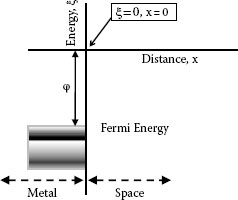
FIGURE 9.10
Potential energy versus distance for an electron near a metal surface.

TABLE 9.4
Thermionic Emission B Values for Some Metals

Contact Material	$B\left(A{\text{cm}}^{-2}{\text{K}}^{-2}\right)$
Ag	60
Au	60
C	6
Cr	50
Cu	65
Mo	85
Ni	30
Pt	32
W	65

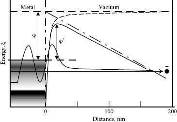
FIGURE 9.11
An illustration of the quantum-mechanical tunneling mechanism by which a field-emitted electron may escape, or tunnel, from the surface of a metal. It shows the modified high-field potential barrier outside the surface (solid line), where the contributions of the image potential and the applied field (E = 3 × 10⁹ V m⁻¹) are shown by the broken and the broken–solid lines, respectively. In addition, the wave function of a tunneling electron is depicted [21].

$J=\left(\frac{B_1{E}^2}{\varphi }\right)exp\left(-\frac{B_2{\varphi }^{3/2}}{E}\right)$

(9.36)

where B_l and B₂ are known fundamental physical constants [20,21]. It is, therefore, possible to liberate electrons from microscopic projections on the cathode. If the voltage imposed across the electrode is high enough for two contacts separated by a distance d in vacuum. It is also possible for these electrons, in turn, to heat the metal below the anode’s surface [20]. Metal vapor is liberated into the contact gap when the current density in a cathode projection causes it to evaporate and/or when the anode’s subsurface reaches it boiling point [20]. The ionization of this metal vapor then results in a breakdown of the contact gap. It is now recognized that the breakdown voltage is very dependent upon the microscopic surface conditions of the cathode. It is thought that for a given metal there is given critical breakdown field given by E_c but the breakdown voltage V_B is given by

$V_{\text{B}}=\frac{E_{\text{c}}d}{\text{β}}$

(9.37)

where β is an enhancement factor which depends upon the geometry of the contacts and the microscopic variations of the cathode surface [20]. Table 9.5 gives values of E_c for a number of metals. Equation 9.37 is only valid for contact gaps less than about 0.3 mm [20]. At longer gaps $V_{\text{B}}\approx K{d}^{1/2}$, where K is a constant [20]. Vacuum breakdown has also been observed between contacts in atmospheric air at room temperature if the distance between the contacts is less than 5–10 electron mean free paths, i.e. d ≤ 10⁻⁵ m. At these small contact gaps Paschen’s law no longer applies. Figure 9.12 shows the dependence V_B of as a function of contact spacing for clean contacts in air [23]. Here $V_{\text{B}}\approx 100d$ (when d is in μm). This relationship is also valid for V_B in vacuum between contacts with a gap of less than about 0.3 mm. The inference is, therefore, that the breakdown process between closely spaced contacts in air at atmospheric pressure is similar to the process that results in the breakdown between contacts in vacuum [23]. It has been shown experimentally for closely spaced, palladium contacts in air [13] that an arc will be initiated if

TABLE 9.5
Critical Vacuum Breakdown Field for Various Metals

Metal	Ec (× 108 Vm−1)	φ (eV)
Cr	53	4.6
Mo	54	4.4
Stainless steel	59	4.4
Au	64	4.8
W	65	4.5
Cu	69	4.5
Ni	104.	4.6

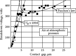
FIGURE 9.12
Breakdown voltage as a function of contact gap in the range 0.2–40 μm [23].

E > 30 × 10⁸ V m ⁻¹ stringently clean contacts

E > 30 × 10⁸ V m ⁻¹ stringently clean contacts

E > 0.5 × 10⁸ V m⁻¹ organically contaminated or activated contacts

Thus, from Figure 9.12 if the circuit voltage is 40 V for clean contacts the arc will be initiated in air at atmospheric pressure with a contact spacing of approximately 4 × 10⁻⁷ m. Once the arc is initiated the pressure from the arc on the contacts may prolong the closing time (e.g., see Figure 13.40). Figure 9.13 puts together the gas breakdown and the small gap breakdown data.

9.3.3    The Volt–Current Characteristics of Separated Contacts

Take the circuit shown in Figure 9.14, where it is hypothetically possible to gradually increase the circuit voltage from zero. When the various states of the breakdown process occur the series resistor permits fine control of the current. The progression of the curve is summarized below [13].

A.  In this region, electrons emitted at the cathode are collected at the anode.

B.  At a certain voltage level all the electrons emitted at the cathode are collected and current saturation is reached. Beyond this point further current increase requires either interaction of the electrons and the gas, or much stronger fields; e.g., fields at the cathode surface that are found for vacuum breakdown.

C.  Electron collisions with the gas between the contacts create additional electron–ion pairs, which increase the current, and this marks the beginning of the breakdown.

D.  When the electron multiplication reaches a critical stage a Townsend avalanche begins.

E.  After breakdown, the current is sustained by the same avalanche mechanism, except that a smaller voltage is required to maintain the necessary ionization. This steady discharge is characterized by a relatively constant voltage drop over about two decades of low current (<10⁻¹ A), a cold cathode and a number of luminous zones. Hence it is called a glow discharge. For any particular gas there is a characteristic sustaining voltage. The voltage also depends upon the cathode material. The principal voltage drop occurs in the space between the cathode and start of the luminous region, called the cathode fall. This voltage is required to produce the discharge sustaining electrons from the cathode by field emission enhanced by secondary emission processes. The glowing region is also characterized by a fairly constant current density, i.e., as the current increases, the cross-sectional area of the glow increases.

F.  When the current increases to the point where the electron emission comes from the entire cathode area, further increase in current leads to higher current density. This leads to joule-heating of the cathode with further increase in electron emission. This region is called the abnormal glow.

G.  Intense cathode heating and the consequent increase in electron emission finally permits the discharge to be sustained at lower voltages. The interaction of the increased number of electrons with the gas forms another avalanche breakdown to form the arc.

H.  The arcing region is one characterized by low voltage and a current only limited by the circuit’s impedance, together with a highly luminous discharge.

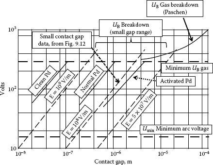
FIGURE 9.13
Combined voltage and contact gap values for long contact gap and short contact gap breakdown [13].

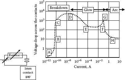
FIGURE 9.14
Voltage–current characteristics for gas breakdown and arc formation between open contacts [13].

9.4    The Formation of the Electric Arc

9.4.1    The Formation of the Electric Arc During Contact Closing

The time required for the establishment of an electrical discharge, after the application of a sufficiently high voltage across open contacts, has been the subject of considerable scientific interest. It is also of great practical importance in contact applications: especially when they are closing.

Once a voltage is impressed across an open contact gap, there are two important time periods. The first is the statistical time lag, t_st. Here the first electron becomes available to begin the breakdown process. The second is the formative time lag t_f. This is the time required for the discharge to become established. The t_f depends upon the over-voltage, the gas, the contact geometry, and the number of initiating electrons [24].

If the threshold voltage for breakdown is V_B and a voltage U > V_B is impressed across the contact gap, then it has shown that

$t_{\text{f}}\propto {\text{θ}}^{-1}$

(9.38)

where $\text{θ}=\left(U-V_{\text{B}}\right)/V_{\text{B}}$. Figure 9.15 shows the compilation of experimental data [24]. From this figure, it can be seen that t_f can range from about 40 ns when $U=2V_{\text{B}}$, 400 ns when U = 1.1 V_B, 4 μs when U = 1.01 V_B and 40 μs when U = 1.001 V_B. Therefore, once the voltage is impressed across the contacts and the first electron is initiated, all the processes discussed in Figure 9.14 can occur very quickly: see for example Figure 9.9. For example, if a contact is closing at 1 ms⁻¹ it only travels 1 μm in 1 μs, so even if the contacts are 10⁻⁴ m apart an arc established between them will burn for 100 μs before they actually touch.

9.4.2    The Formation of the Electric Arc During Contact Opening

If the circuit current is greater than a minimum value and the voltage that appears across the opening contacts is also greater than a minimum value (see Section 9.5.4), an arc will always form between them. The arc formation depends entirely upon the properties of the contact material and the arc always initiates in metal vapor from the contacts themselves. From Chapter 1 (Equation 1.11) the contact resistance R_c is given by

$R_{\text{c}}=\frac{\text{ρ}}{2a}=\frac{\text{ρ}}{2}\sqrt{\frac{\text{π}H}{F}}$

(9.39)

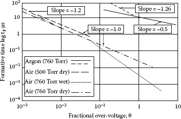
FIGURE 9.15
Plots of formative time lag, t_f, versus fractional over voltage using data supplied by a number of researchers [24].

where ‘a’ is the radius of the real area of contact, H is material hardness, ρ is resistivity and F the holding force. As the contact begin to open F → 0 and so a → 0 and so R_c will increase. As R_c increases, U_c, the voltage drop across the contacts, given by

$U_{\text{c}}=IR$

(9.40)

also increases. Chapter 1 (Equation 1.40) also showed that the temperature of the contact spot T_c will increase because

$T_{\text{c}}^2=T_0^2+U_{\text{c}}^2\times {10}^{7}K$

(9.41)

where T₀ is the ambient temperature. A stage will be reached when the temperature of the contact spot equals the melting point, T_m, of the metal [25]. Figure 9.16 compares calculated values of U_c at T_m with measured values for a wide range of metals used as electric contacts. Table 9.6 gives values taken from Holm [14]. Once the contact spot has melted and the contacts continue to part, they draw a molten metal bridge between them. This molten metal bridge always forms between the contacts even at low currents [26,27,28,29], even when the contacts open with a very slowly [28] or with high acceleration [26,30,31], and even when they open in vacuum [32,33]. For example, Figure 9.17 shows three voltage traces of molten metal bridges forming between Au contacts in a 10 mA, 4 V circuit [29] and Figure 9.18 [27] shows the length of the molten metal bridge over the current range 1 to 79 mA. The molten metal continues to bridge the opening contacts until it becomes unstable and ruptures. After the rupture of the molten metal bridge an arc forms in its vicinity. A typical change in the initial voltage drop across the contacts is shown in Figure 9.19. Figure 9.20a–c shows examples of the measured voltage as the contacts open and form the molten metal bridge, as the bridge ruptures and the arc is initiated between three different contact materials and for a wide range of currents: 20–1,000 A and three different contact metals [30,34,35].

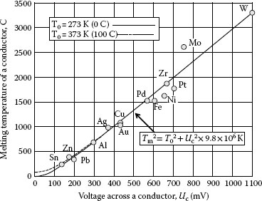
FIGURE 9.16
Relationship between the measured voltage drop across a conductor and its calculated and measured melting temperature.

TABLE 9.6
Melting Voltages for Various Metals

Metal	Melting Temperature (K)	Measured Melting, Um (V)
W	3,683	1.1
Mo	2,883	0.75
Ni	1,726	0.54
Cu	1,356	0.43
Au	1,336	0.43
Ag	1,234	0.37
Al	933	0.3
Pt	2,042	0.71

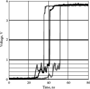
FIGURE 9.17
The voltage characteristics of molten metal bridges from three openings of Au contacts in a 10 mA, 4 V circuit[29].

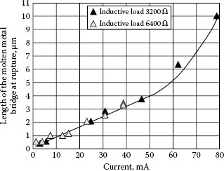
FIGURE 9.18
The length if the molten metal bridge for currents in the range 1–79 mA [27].

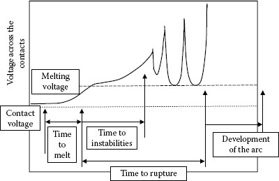
FIGURE 9.19
The initial voltage drop across a pair of closed electrical contacts as they begin to open.

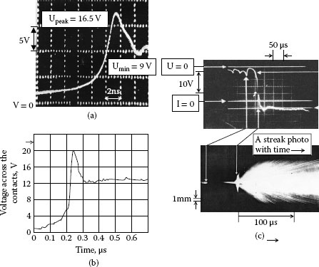
FIGURE 9.20
Actual initial voltages across contacts opening over three different contact materials and a wide range of currents; (a) Au contacts, 20 A[dc], 6 V [35], (b) Cu contacts, 50 A[dc], 100 V [34] and (c) Ni contacts, 1,000 A[ac], 440 V [30].

These voltage characteristics can be described using the four stages shown in Figure 9.21 [36,37]:

Stage (a): Once the molten metal bridge has formed its rate of change of voltage is about 2 × 10³ V s⁻¹. As the contacts continue to open and the bridge is drawn further it becomes unstable. There are a number of physical reasons for this instability, including surface tension effects, boiling of the highest temperature region, convective flows of molten metal resulting from the temperature variation between the bridge roots and the high-temperature region. Figure 9.20c shows this instability for Ni contacts opening a current of 1,000 A. The streak photograph of this opening shows that the unstable bridge is incandescent (i.e. >2,900°C). In this case the high temperature results in more metal entering the bridge and it cools. The bridge will eventually rupture, releasing metal vapor into the contact gap when the voltage across it, U_b, is close to the calculated boiling voltage U_b1 of the contact materials, i.e.:

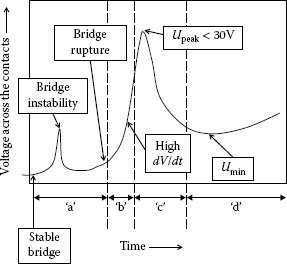
FIGURE 9.21
The four stages of molten metal bridge rupture and metal phase arc formation.

TABLE 9.7
Comparison of the Boiling Voltage (U_bl) with the Break Voltage (U_b) for Various Metals

Metal	Breaking Voltage (Ub)	Calculated Boiling Voltage (Ubl)	Boiling Temperature Tbl(K)
Ag	0.75	0.77	2,485
Cu	0.8	0.89	2,870
W	1.7	1.82	5,800
Au	0.9	0.97	3,090
Ni	1.2	0.97	3,140
Sn	0.7	0.87	2,780

$U_{\text{b}}=\sqrt{L\left(T_{\text{bl}}^2+T_0^2\right)}$

(9.42)

where L is the Lorenz constant and T_bl K is the boiling temperature see Table 9.7.

Stage (b): Once the bridge ruptures the voltage across the contacts rises very rapidly without a discontinuity from about 10³ V s⁻¹ to about 10⁹ V s⁻¹: at 10 mA for Au contacts $\text{d}V/\text{d}t\approx 0.5\times {10}^9\text{V}{\text{s}}^{-1}$ [29], at 150 A for Cu contacts $\text{d}V/\text{d}t\approx 5\times {10}^9\text{V}{\text{s}}^{-1}$ [34], at 1 kA for Cu contacts $\text{d}V/\text{d}t\approx {10}^9\text{V}{\text{s}}^{-1}$ [31] and for Ni contacts $\text{d}V/\text{d}t\approx 2\times {10}^9\text{V}{\text{s}}^{-1}$ [31]. This rate of rise of the voltage will depend upon the dimensions of the molten metal bridge just before its rupture. After the bridge rupture a very high pressure, perhaps as high as 100 atmospheres [36,37], very low electrical conductivity, metal vapor exists between the contacts. This region can then be considered to be a capacitor with a very small capacitance. Because the circuit’s inductance prevents a rapid change in current (see Figure 9.20c), charge flows from the circuit inductance into this small capacitor causing the very high dV/dt. The metal vapor volume expands rapidly into the surrounding lower pressure ambient and as it does its pressure also decreases rapidly. When the pressure of the metal vapor decreases to 3–6 atmospheres conduction is initiated with a voltage across the contacts of a few 10’s of volts, see Figure 9.20. At these pressures the discharge that forms is the “pseudo arc” [38,39] where the current is conducted by ions. During this stage the electrons required for charge neutrality will be introduced into the discharge from secondary emission resulting from ion impact at the cathode. As the original molten metal bridge will have material from both the cathode and the anode, net transfer of material from the anode to the cathode is expected and is indeed observed [36,37]: see Section 10.3.5. At this stage radiation from neutral Cu (CuI radiation) is observed during the initial rapid rise of the voltage, but ionized Cu radiation (CuII radiation) is not observed, see Figure 9.22a and b [34]. Once the pseudo arc forms there is a large increase of the CuI radiation and a slowly rising increase of the CuII, see again Figure 9.22 a and b.

Stage (c): As the pressure of the metal vapor continues to decrease to about 1–2 atmospheres, the pseudo arc transitions into the usual arc discharge with an arc voltage impressed across the contacts whose value is about that of the minimum arc voltage expected for an arc operating in the contacts’ metal vapor (i.e., U_min ≈ 10–20 V, see Section 9.5.4). Here again net material transfer will be from anode to cathode (see Section 10.3.5). Thus all arcs formed between opening contacts in all ambient will operate in metal vapor and only transition to one operating mainly in the ambient gas as the contacts continue to open (see Section 10.3.5). It is only in a vacuum ambient that the arc continues to operate in metal vapor evaporated from the contacts themselves [20,32,33]. In order to sustain this arc a minimum arc current is also required (see Section 9.5.4).

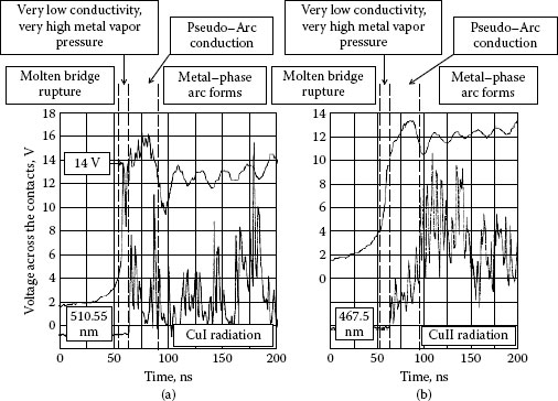
FIGURE 9.22
The transition from molten metal bridge to the metal phase arc [34]: (a) Voltage, neutral copper radiation (Cu I), Cu contacts, 50 A, 100 V and (b) voltage, ionized copper radiation (Cu II), Cu contacts, 50 A, 100 V.

Stage (d): At this stage as the contacts continue to open the arc between them gradually transitions from the metallic phase arc to the ambient, gaseous phase arc with most of the current now carried by electrons. Once the metallic phase arc forms there is a large increase in the CuII radiation, see Figure 9.22b. The whole sequence is illustrated in Figure 9.23. As the contacts continue to open this metallic phase arc transitions into an arc operating in the ambient atmosphere (see Section 10.3.5). The parameters required to form and sustain an arc are summarized in Table 9.8.

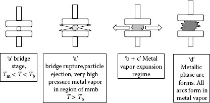
FIGURE 9.23
The opening sequence of an electric contact; formation of the molten metal bridge, its rupture and arc formation.

TABLE 9.8
Parameters Required to Form and to Sustain an Arc

Condition	Voltage Across Contacts	Circuit Current
To Initiate Breakdown
Gas breakdown: No conduction to glow	${\text{V}}_{\text{B}}\left(gas\right)\approx >329+3\times {10}^6\times d$ for air (d in m.)	$I\approx >10<600\text{mA}$
No conduction to stable or unstable arc	For air at atmospheric pressure	I ≈ > 20 mA
Small gap or vacuum breakdown for U ≤ UB(gas)	VB (vacuum) > Ecd: i.e., ≈ > 108 d $E_{\text{c}}\approx 0.5\times {10}^8{\text{Vm}}^{-1}$ “activated” contacts $E_{\text{c}}\approx 2.0\times {10}^8{\text{Vm}}^{-1}$ “normal” contacts $E_{\text{c}}\approx 30\times {10}^8{\text{Vm}}^{-1}$ “clean” contacts	A critical pre-breakdown emission current: I ≈ > 50 mA to 1.0 A I ≈ > 1 A in vacuum
Conduction to arc stable or unstable		I ≈ > 50 mA in Air
To Sustain Breakdown
Glow (gas dependant)	$V_{\text{G}}\left(\text{gas}\right)=280+{10}^6\times d$ for Air (d in m.)	$I_{\text{G}\left(\min \right)}\approx >10\text{mA}$
Arc (contact material dependant)	$V_{\text{A}}=V_{\text{m}}+P\times {10}^{3}d$ where P ranges from 1 to 10 and is $f\left(I\right)V_{\text{m}}$ ranges from 10 to 20 V is f (metal and I)	$I_{\min }=0.5\text{A}\text{to}\text{1}\text{.0A}$ (metal surface condition)
To Initiate and Sustain Arc During Contact Opening
Contact opening	$V_{\text{A}}\ge V_{\text{m}}$	$I_{\min }=0.5\text{A}\text{to}\text{1}\text{.0A}$ (metal surface condition)

9.5    The Arc in Air at Atmospheric Pressure

This section will concentrate upon the arc in air at atmospheric pressure, because this is the arc that the vast majority of switching contacts experience. It occurs during the closing and opening of most relays, contactors, switches, and circuit breakers that operate in air. There are some high-voltage circuit breakers and contactors that use the gas such as H₂ and SF₆ [17] or operate under oil (i.e., high-pressure H₂). The general description of the arc in air also applies to the arc in any high-pressure gas including SF₆ and H₂. The other form of arc is the so-called vacuum arc, which occurs in a special class of interrupters where contacts operate in a high-vacuum environment [20]. The vacuum arc does exhibit special characteristics different from the arc in air and will be described briefly in Section 9.6.

A generic arc is shown in Figure 9.24 together with its voltage characteristic. There is a voltage drop at the cathode (U_c between 8 and 20 V) and almost always another voltage drop at the anode (U_a between 1 and 12 V). These regions are known as the cathode fall and the anode fall respectively. They occur over very short distances from the open contact surfaces, so that the electric fields in these regions are very high. In between them is the arc column.

9.5.1    The Arc Column

The arc column has the characteristics of the plasma discussed in Section 9.2. The density of the electrons, n_e, equals the density of the ions, n_i. At atmospheric pressure, there is local thermodynamic equilibrium, i.e.,

$T_{\text{e}}\left(\text{electron}\text{temperature}\right)=T_{\text{i}}\left(\text{ion}\text{temperature}\right)=T_{\text{g}}\left(\text{gas temperature}\right)$

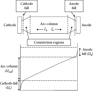
FIGURE 9.24
Schematic of an arc with the column constricted at the contacts with the corresponding voltage distribution (note: the length of the cathode and anode sheath regions are not to scale).

For the low-current, free-burning arcs (approximately 5 A), T_g is between 6,000 and 7,000 K and the temperature for high-current, free-burning arcs (approximately 1,000 A) is about 20,000 K. It is unusual in free-burning arcs to obtain a temperature much higher than this value, thus the average energy of the ions and gas atoms in arcs has a range from about 0.85 eV for low-current arcs to about 2.5 eV for high-current ones. The arc temperature can be determined spectroscopically [40]. Figure 9.25 shows the temperature profile of a 1,000 A, free-burning arc between Cu contacts [41]. The current density in the arc core is

$J=\left(n_{\text{e}}e{M}_{\text{e}}+n_{\text{i}}e{M}_{\text{i}}\right)E$

(9.43)

where M_e and M_i are the electron and ion mobilities and E is the column’s electric field strength. Since, $M_{\text{e}}\gg M_{\text{i}}$, greater than 99% of the current in the arc column is carried by electrons. The ion concentration in the ac column at atmospheric pressure can be calculated using a simplified form of Saha’s equation [9,42,43]:

${\log }_{10}\frac{n_i^2}{n}=-5400\frac{V_i}{T}+\frac{3}{2}{\log }_{10}T+15.385$

(9.44)

where V_i is ionization potential of the gas, $n=n_{\text{n}}+n_1$ (n_n density of the neutral atoms). In most arcs between metal contacts that are far enough apart, there is a mixture of the atmospheric gases and metal vapor from the contacts. The gas having the lowest ionization potential in the mixture is the most readily ionized. As most metal vapors have much lower ionization potentials than nitrogen or oxygen, any metal vapor in the air will be preferentially ionized. The metal vapor concentration can also be calculated using the Saha equation together with a spectroscopic analysis of the arc [41]. In recent years the arc column has been modeled very successfully using the calculating power of computers [44]. The use of suitable software to design and analyze switching devices will be discussed in Chapter 14. A simple, steady state, arc model given by Elenbaas [45] and Heller [46] has found wide use to explain arcing phenomena. This model is illustrated in Figure 9.26. Here the energy input is given by the current flowing in the column times the voltage drop (i.e., Joule heating), is only balanced by the radial thermal losses and radiation, i.e.:

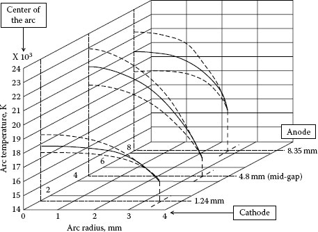
FIGURE 9.25
Temperature profile for a 1,000 A free-burning arc in air between copper contacts [41].

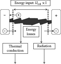
FIGURE 9.26
The Elenbaas–Heller arc model.

$\text{σ}{E}_{\text{col}}^2=\frac{1}{r}\frac{d}{dr}\left(r\text{κ}\frac{\text{d}T}{\text{d}r}\right)+P_{\text{r}}$

(9.45)

where r is the arc radius, κ thermal conductivity, P_r the radiation loss, σ the electrical conductivity and E_col is the column’s electric field. Using this equation it is possible to determine at least qualitatively how an equilibrium arc will behave.

Example 1: The low current arc (1–30 A): here, using Lowke’s analysis [47], it is possible to determine how the arc radius and the arc voltage vary as a function of current. In this current range, the controlling physical process is natural convection. For a vertical arc, the electrical energy going into the arc plasma is carried upwards by natural convection. The integrated flow of enthalpy across any arc cross section can be considered equal to the total electrical energy upstream of the axial position being considered. Thus, the arc radius will increase as a function of the distance from the lower contact.

If we assume the arc temperature as a function of arc radius is parabolic, i.e.

$T\left(r\right)=T_{\text{mx}}-D{r}^2$

(9.46a)

where T_mx is the maximum arc temperature at r = 0 and D is a constant. Substituting in Equation 9.45

$T\left(r\right)=T_{\text{mx}}-\frac{\text{σ}{\left(E_{\text{col}}\right)}^2{r}^2}{4\text{κ}}$

(9.46b)

Then neglecting the temperature at the arc boundary and if the arc temperature is assumed to be determined primarily by the energy balance at the arc center then:

$\frac{I^2}{\text{σ}{A}^2}=\frac{4\text{πκ}{T}_{\text{mx}}}{A}+P_{\text{r}}$

(9.46c)

where $\text{σ}{\left({\text{E}}_{\text{col}}\right)}^2$ is expressed in terms of the current using Ohm’s law $I=\text{σ}{\text{E}}_{\text{col}}A$ and A is the arc area. Lowke [46] showed that if the radiation losses were negligible, then the arc radius r and the arc voltage U at a height z above the lower contact are given by:

$r=\frac{0.56}{{\left(\text{δ}\hslash \text{σ}\right)}^{1/4}}\left(\frac{\text{σ}z}{{\text{δ}}_{\text{b}}g}\right)I^{1/2}$

(9.46d)

$U={\displaystyle \int E\text{dz}}=1.37{\left(\frac{\text{δ}\hslash }{\text{σ}}\right)}^{1/2}\left(\frac{{\text{δ}}_{\text{b}}g}{\text{δ}}\right)z^{3/4}$

(9.46e)

where δ is the average arc plasma density, δ_b, is the density of the gas at the arc boundary, and ℏ is the enthalpy. Calculating the value of U as a function of I over this current range gives the familiar negative volt–ampere characteristic that will be discussed in Section 9.5.5. It is interesting to note that, as the arc radius (and hence the arc area) increases as the current increases, then at least qualitatively, one would have expected from Ohm’s law that the arc voltage would decrease.

Example 2: Assume the cooling rate at the arc boundary is increased while the current is kept constant. This is commonly done in practical circuit breakers and dc contactors (see Chapter 14). The arc will respond by reducing its diameter, because the conducting radius of the gas will have decreased. Because the arc current remains constant, the current density will increase, i.e., J = σE will increase and the power density σE² will also increase. The increase in the power density will increase the temperature of the arc. Thus, in order to satisfy the Elenbaas–Heller equation, the temperature gradient at the arc boundary will increase at a faster rate than the decrease in arc diameter. As soon as an equilibrium state is reached, the consequence of cooling the outer edges of the arc will be at a higher temperature than at the arc’s center.

Example 3: A higher thermal conductivity will also tend to increase the radial heat loss from the arc, and the arc will again respond with a smaller diameter and higher peak temperatures. This effect of gas with different thermal conductivities on arc diameter is well illustrated in Figure 9.27 [48].

Example 4: The high current arc (>100 A): here the arc properties are also largely determined by convection, but at these currents the convection is driven by the self magnetic field generated by the current flowing in the arc. Other physical processes also become more dominant as the arc current increases: radial pressure gradients become significant; radiation losses dominate at the arc center; viscous and turbulent forces can result in further energy losses. Lowke [48] analyzed of these effects and developed the positive volt-ampere characteristic observed for high current arcs, see Section 9.5.5. The self-magnetic also causes a drastic reduction in arc radius as the current increases from ~50 A to ~1,000 A, see Figure 9.28.

9.5.2    The Cathode Region

The cathode contact provides the electrons, the fuel that allows the arc to continue burning between the contacts. If the source of electrons from the cathode is terminated, then the arc will extinguish. The cathode region illustrated in Figure 9.29 is usually characterized by having high electric fields of 10⁸–10⁹ V m⁻¹, high thermal gradients (e.g., see Figure 9.25), contraction, i.e., the current density is higher than that of the arc column (maybe as much as 100 times greater) and at high currents, plasma jets [9] can form in this region. Two separate descriptions of electron emission have been observed, the first on refractory metals with high melting points such as tungsten. These readily emit electrons when heated to a temperature less than the melting point of the metal. The current density is given by the Richardson–Dushman equation, see Section 9.3.2, Equation 9.34. Most practical contact systems, however, use metals that boil at temperatures well below the temperature required to produce enough electrons to sustain the arc. Many researchers have studied the possible mechanisms to product the electrons from so called “cold cathodes.” An excellent review is presented by Guile [50]. A interesting description and model of the cathode fall for tungsten contacts (i.e. thermally emitting contacts) is given by Zhou et al. [51]. However, as Kesaev [52] remarked …

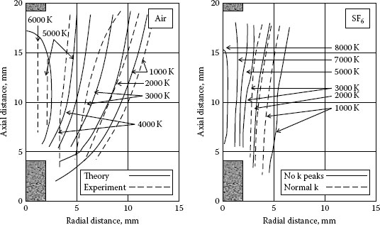
FIGURE 9.27
Temperature profiles for free burning 10 A arcs in air and SF₆ [47].

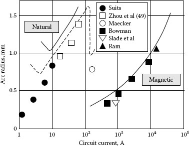
FIGURE 9.28
The radius of a free-burning arc column as a function of current [48].

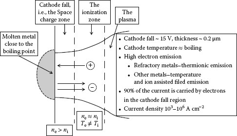
FIGURE 9.29
The cathode region of the arc.

this branch of physics is a collection of a large number of isolated pieces of work conducted under conditions difficult to compare and, as a rule, giving equivocal results.

In general, there is a consensus that the electron emission from “cold cathodes” involves a combination of thermally enhanced field emission (called T–F emission) and the effects of ion bombardment [12,53,54]. In the cathode fall region only about 90% of the current is carried by electrons, so 10% is carried by the ions.

There must be an energy balance at the cathode. Among the components that supply energy are:

1.  Thermal energy from ions and neutral atom bombardment

2.  Kinetic energy from ions dropping through the cathode fall

3.  Condensation of ions and neutral atoms on the cathode

4.  Radiation from the arc plasma

5.  Chemical reactions in the cathode surface

6.  Joule-heating of the cathode

Among the components that cause energy loss are:

1.  Energy for electron emission which is approximately $eU\phi$ for each thermionically emitted electron but is zero for each electron emitted by pure field emission. For cold cathodes the energy loss is somewhere in between.

2.  Evaporation of cathode material.

3.  Ejection of metal globules and particles.

4.  Radiation from cathode surface.

5.  Dissociation of molecules at the cathode surface.

6.  Heat conduction by the bulk metal of the cathode contact.

7.  Heat conducted or convected away by the surrounding gas.

In Figure 9.30, Cobine illustrated typical energies involved in some of these mechanisms [55].

9.5.3    The Anode Region

The anode region shown in Figure 9.31 can be either active or passive. In the passive mode, it serves only to collect the electrons carrying the current from the arc column. A space charge in front of the anode accelerates electrons from the column (i.e. n_e ≠ n_i). If, however, the thermal boundary layer between the arc column and the anode surface is small enough and the electron density gradients are high enough so that a substantial electron diffusion flow exists, then a space charge region is unnecessary. The anode fall voltages can thus range from close to zero to as high as 15–20 V. In most of the arcs which exist for times >1 ms between opening contacts with currents higher than a few amperes, an anode fall will exist with fields between 10⁸ and 10⁷ V m⁻¹ and the anode fall thickness will be 10⁻⁴ to 10⁻⁶ m. An excellent review of the anode fall region is presented by Heberlein et al. [56]. Although much of their analysis is for arcs in an argon ambient, the general principles they present are relevant for arcs in air and other gases. The components that supply energy at the anode are:

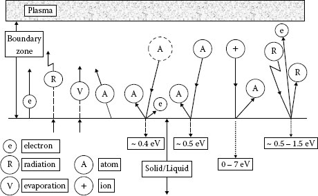
FIGURE 9.30
Possible mechanism of energy transfer at the cathode and/or anode [55].

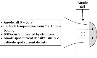
FIGURE 9.31
The anode region of the arc.

1.  Thermal energy from neutral atom bombardment

2.  Kinetic energy from the electrons dropping through the anode fall

3.  Condensation of neutral atoms on the surface

4.  Radiation from the arc plasma

5.  Chemical reactions on the anode surface

6.  Joule-heating of the anode

7.  The energy gained by entering electrons from the work function, which is approximately $eU\text{φ}$

These are balanced by:

1.  Evaporation of anode material

2.  Ejection of globules and particles

3.  Radiation from the anode surface

4.  Dissociation of molecules at the anode surface

5.  Heat conduction into the bulk of the contact

6.  Heat conducted or converted away by the surrounding gas

9.5.4    The Minimum Arc Current and the Minimum Arc Voltage

Once an arc has been established between opening contacts, it requires a continuous supply of electrons from the cathode to sustain it. These electrons will only be liberated in sufficient quantity if the cathode temperature remains high enough to liberate thermionic electrons for refractory contacts, or to liberate electrons by T–F emission for low melting point contacts. These electrons will ionize the metal vapor that the arc initially forms in. Intuitively it is reasonable to assume that if the arc current drops below a minimum value, i.e.,

$I_{\text{A}}\le I_{\min }$

(9.47)

the energy losses discussed in Section 9.5.2 will exceed the energy input to the cathode and electron production will cease, causing the arc to be extinguished or if the current is low enough the arc may not form at all after the rupture of the molten metal bridge. Detailed experiments on opening contacts for currents less than 1 A using oscilloscopes with a high frequency resolution by Ben Jemma et al. [57,58,59,60] and extended by Hasagawa et al. [61,62,63] have shown that the definition of I_min needs to be revised. Figure 9.32 shows that an arc discharge can occur between Ag contacts at currents well below the former I_min of 0.4 A given in Table 9.9. This figure shows that the actual arc duration at any given current has considerable variation. While the average variation with current is generally linear, there is a transition close to 0.5 A where the slope increases. Figure 9.33 gives the average arc times for five different contact materials. Examples of the measured voltage wave forms across Ag contacts show three separate regimes, Figure 9.34. (A) Where no arc occurs and a voltage transient determined by the inductance and capacitance in the circuit. (B and C) Here a short duration arc is seen with a voltage close to the expected minimum value, U_min. This discharge is unstable and ‘chops’ out without reaching a value close to the circuit’s emf (see the requirements for interrupting a dc circuit in Section 9.7.2). Because the current chops to zero in this way, there is still current trapped in the circuit’s inductance. Thus the voltage wave form after the arc has extinguished is similar to that shown in (A) and depends upon the residual current and the circuit’s inductance and capacitance. This unstable condition is seen more clearly at higher currents for an arc between contacts opening in vacuum and is there termed “The chop current” [20]. (D to F) At these currents a stable arc forms in the metal vapor from the ruptured molten metal bridge. It operates until the arc voltage has driven the circuit current down to a value where the arc can no longer exist. The resulting voltage wave form after the arc has extinguished still shows the oscillations that you see in (A) and (B and C). As the circuit current is reduced arcing only occurs 100% of the time for currents greater than a given value which is strongly dependent upon the contact material, see Figure 9.35. Ben Jemma used this result to define as I_min the current above which an arc occurs 100% of the time. The values of this I_min are compared to the traditional values in Table 9.9. The lowest current that arcing can occur I_lim will be much lower than this I_min. For switch designers it is important to note that contact erosion and a change in the contact surface resulting from the electric arc will occur at currents well below the I_min value. The duration and stability of these short duration arcs show a strong dependence upon the contacts’ opening speed, the circuit’s inductance and the circuit’s dc emf [58,59,60,61,62,63]. Note that this discussion of I_min is only valid for the initial contact opening. After the molten metal bridge has ruptured the arc forms in metal vapor between very closely spaced contacts. The energy loss in this arc is mostly through thermal conduction, with a very small percentage lost through radiation. When opening higher currents, when the arc column is longer, the arc can become unstable at currents higher than the I_min discussed here. This will be discussed in Section 9.7.2

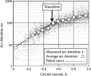
FIGURE 9.32
The arc duration for Ag contacts opening a 14 V dc circuit as a function of current, showing the wide statistical distribution of the measured values [57,58,59].

TABLE 9.9
The Minimum arc Voltage (U_min) and Minimum Arc Current (I_min) and Limiting Arc Current (I_lim) for Various Contacts and Comparison of U_min with Sum of the Ionization Potential V_i and the Work Function Potential $U\text{φ}\left(\text{i}\text{.e}\text{.}{V}_{\text{i}}+U\text{φ}\right)$

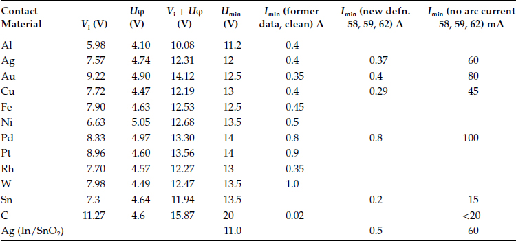
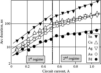
FIGURE 9.33
The average arc duration as a function of current for five different contact materials opening a 14 V dc circuit [57,58,59].

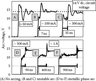
FIGURE 9.34
Measured voltages across opening Ag contacts as a function of current a 14 V dc circuit: (A) no arcing, (B) and (C) a low voltage unstable arc and D–F, the formation of the metallic phase arc [57,58,59].

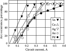
FIGURE 9.35
The probability of arc formation for currents less than 0.6 A for five different contact materials a 14 V dc circuit [57,58,59].

Also it is reasonable to assume that a minimum voltage is required across the open contacts to sustain the arc. The arc would require at least a voltage, U_min, that corresponds to the work function voltage,Uφ, of the cathode contact and the ionization potential of the gas, V_i. Thus,

$U_{\min }\approx V_{\text{i}}+U_{\text{φ}}$

(9.48)

Table 9.9 compares measured U_min with $V_{\text{i}}+U_{\text{φ}}$ for low current arcs between contacts made from a number of different metals. This table also presents values for I_min. If a contact becomes contaminated with carbon deposits (this is called “activation”, Section 9.2.3) then the I_min could decrease to a value you would associate with carbon contacts. Figure 9.36 [64] and Table 9.8 [13] summarize the parameters required to form and sustain an arc.

9.5.5    Arc Volt–Ampere Characteristics

A great deal of data has been developed to show how the arc voltage varies with arc current for a given contact gap. For low dc currents the arc voltage has the negative characteristic shown in Figure 9.37. It tends to go asymptotic at I_min and U_min [14,65,66,67]. Actual data for Cu and AgCdO contacts are shown in Figures 9.38 and 9.39. These curves show us negative volt–ampere characteristic, i.e., as the current in the arc increases, so the voltage drop across the arc decreases. The total arc voltage U_A is given by (see Figure 9.24)

$U_{\text{A}}=U_{\text{c}}+U_{\text{col}}+U_{\text{a}}$

(9.49)

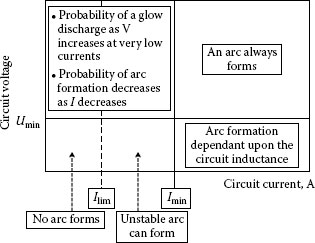
FIGURE 9.36
Voltage and current ranges required to sustain an arc.

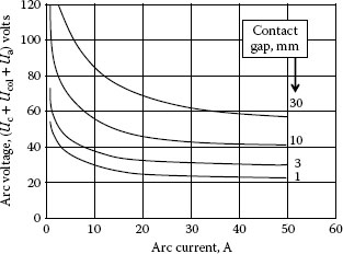
FIGURE 9.37
Voltage-current characteristics for a free-burning, low current dc arc between copper contacts, showing the effect of contact gap.

The form of U_col is complicated by the fact that the arc column usually tends to constrict as it gets closer to the cathode and anode. Figure 9.40 shows the measured total arc voltage U_A as a function of contact gap [68].

Here

$U_{\text{A}}=\text{Δ}+\left(\text{τ}+d\right)E\left(I\right)$

(9.50)

where d is the arc length and I the arc current.

$E\left(I\right)=b{\left(\frac{\ln I}{q}\right)}^{-3}$

(9.51)

and Δ = 26 V, τ = 1.1 cm (for silver contacts), 1.3 cm (for copper contacts) and 1.6 cm (for tungsten contacts), b = 5,400 V cm ⁻¹ q = 7.4 × 10⁻³ A.

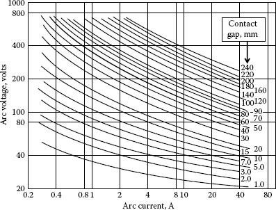
FIGURE 9.38
Voltage–current characteristics for a free-burning, low current dc arc between copper contacts as a function of the contact gap [65].

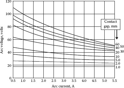
FIGURE 9.39
Voltage–current characteristics for a free-burning, low-current dc arc between AgCdO contacts, as a function of contact gap [66].

At higher currents the arc voltage levels out and then increases as a function of current. Figure 9.41 shows the how arc’s gross electric field (i.e. V/d) varies over 8 decades of current [69]. Lowke modeled the arc voltage 1 cm above the cathode and compared it to experimental data; this is shown in Figure 9.42 [48] (see also Examples 1 and 4 in Section 9.5.1). The important aspect of these data is to note that the arc voltage is not a function of the system or circuit voltage, but instead is determined by the power input required to sustain the arc.

Because the energy stored in the arc is associated with its conductance and with finite rates of energy flow, the arc conductance cannot respond instantaneously to current changes. The conductance and arc voltage tends to lag behind changes in current [70,71]. The degree of lag depends upon the rate of change in arc current and the electrical inertia of the arc, called the arc’s time constant. In Figure 9.43, the effect of different ac frequencies is illustrated. The frequency f₁ is low enough that the static arc voltage–current characteristic is followed; f₄ on the other hand is so fast that the arc conductance cannot follow the current at all and it shows a resistive characteristic. Frequencies f₂ and f₃ have intermediate values [72]. In the case of alternating power frequency arcs (50 or 60 Hz), in the range of ~10 A to a few hundred amps, the arc voltage tends to remain constant during each current half cycle, because the arc in a regime where the arc voltage does not appreciably vary with current (see Figure 9.41). It is only near current zero where an increase in voltage may be observed.

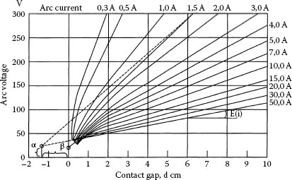
FIGURE 9.40
Arc voltage as a function of contact gap (or arc length) for a free-burning arc in air [68].

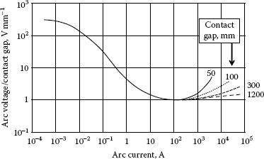
FIGURE 9.41
Voltage–current characteristics as a function of contact gap in air for currents in the range 10⁻⁴–10⁴ A [69]).

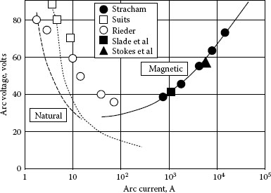
FIGURE 9.42
Voltage–current characteristic for a free-burning arc in air [48].

FIGURE 9.43
f₁ is the static dc arc characteristic and f₄ is the characteristic for a resistance obeying Ohm’s law; the dynamic arc characteristics change from f₁ to f₄ as the frequency of the current increases. Here $f_1<f_2<f_3<f_4$ [71].

9.6    The Arc in Vacuum

A complete description of the vacuum arc, the name given to the arc which is formed between contacts that operate in a vacuum, is given in Reference [20]. The vacuum arc is an arc that forms in metal vapor evaporated from the contacts themselves. It can be formed either from vacuum breakdown of an open contact gap (see Section 9.3.2) or during contact parting by the rupture of the molten metal bridge (see Section 9.4.2). After the rupture of the molten metal bridge, a high-pressure column arc is formed called the bridge column [20,72,73] which can persist for times greater than half a millisecond, see Figure 9.44.

9.6.1    The Diffuse Vacuum Arc

After the bridge column stage the vacuum arc exists in essentially two forms: (1) diffuse and (2) columnar. For currents up to approximately 5 kA, the vacuum arc is diffuse [73,74] and can be characterized by a multiplicity of rapidly moving cathode spots (the number of spots being approximately proportional to the current and dependent on the contact material), a diffuse inter-contact plasma, and a diffuse collection of current at the anode (see Figure 9.45). These cathode spots are essential to the maintenance of the discharge. Most of the arc voltage drop occurs across a space-charge sheath at the cathode. The maximum current conducted by each of the multiple cathode spots varies with the contact material, and is related [20,75,76] to the thermal parameter T_bκ^1/2 of the cathode, where T_b is the normal boiling-point temperature of the contact material, and κ is its low-temperature thermal conductivity. The current density at the cathode surface of an individual cathode spot is extremely high, and this region is therefore one of high power density. For arcs on copper contacts, the cathode fall is approximately 18 V, the maximum current per cathode spot is approximately 100 A, and the cathode spot current density at the surface, based on crater sizes, is 10⁸ A cm⁻² [77,78].

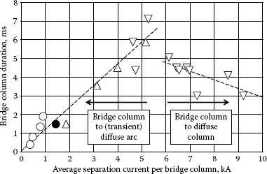
FIGURE 9.44
Duration of the bridge column formed after the rupture of the molten metal bridge for Cu–Cr contacts opening in vacuum [20, 73].

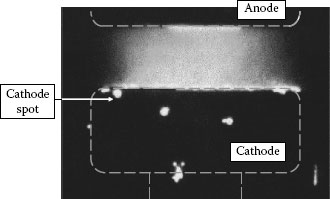
FIGURE 9.45
The diffuse vacuum arc.

All the material required to maintain the arc comes from the cathode spots. Of particular importance is the fact that the cathode spots are regions of intense ionization [20,52,75,79]. It is in this region that both ions and electrons are produced, both of which move away from the cathode spot with high energy. For current levels of several hundred amperes, the ion flux leaves the cathode spots with a spatial distribution approximating a cosine law [80,81,82,83]. For higher current levels, the ion flux more closely approximates an isotropic distribution [84]. Metal particles also stream away from the cathode spot regions, primarily in a direction parallel to the cathode surface [81]. For copper arcs, the erosion rate is about 10⁻⁴ g C⁻¹ and, in common with most materials, the magnitude of the ion current leaving the cathode spot region is about 10% of the arc current [20,78,84]. The ions possess an energy (in electron volts) which exceeds the arc voltage [85,86]. Energies of 50–100 eV have been measured for the metals commonly used in vacuum interrupter contact materials. Initially it was proposed that the ions migrated away from a localized potential maximum [85,86,87,88] within the cathode spot. It now seems probable that this ion acceleration results from a force on the ions from the very high pressure gradients within the cathode spot coupled to some extent with an electron-ion friction effect [20,79,89]. The ions are multiply charged [86,87,89,90] and possess a mean energy approximately 20–40 eV (with velocities about 10⁶ cm s⁻¹), whereas the mean energy of the neutral metal vapor is less than 1 eV. Figure 9.46 illustrates the complex cathode spot of the diffuse vacuum arc [20].

The primary cathode spot parameters that influence successful interruption at current zero are (1) the high velocity of the ionized metal vapor away from the cathode surface, which leads to a rapid decrease in the inter-contact plasma density, and (2) the absence of a cathode spot at the new cathode (see Section 9.7.3).

For certain arcing conditions, there may be significant evaporation from the anode due to the formation of a single, grossly evaporating anode spot [91]. This anode spot operates near the normal boiling temperature of the anode material, and can significantly increase the inter-contact plasma density. Furthermore, since the erosion is not distributed, anode spot formation can cause gross melting of the contact. Finally, a plasma jet from the anode spot can cause the cathode spots to bunch together [92], with resulting gross erosion on the cathode.

Anode spots can form from an initially diffuse vacuum arc. The probability of anode spot formation [92,93] increases with increasing contact separation, with increasing circuit current and arc duration, and with decreasing anode area. Furthermore, the probability of spot formation increases with a decrease in the anode thermal parameter $T_{\text{m}}{\left(\text{κδ}{C}_0\right)}^{1/2}$, where T_m is the melting temperature of the anode material and κ, δ, and C₀ are the thermal conductivity, density, and specific heat respectively. For small anode areas and long contact spacing, when most of the ions in the plasma stream from the cathode spots are no longer incident on the anode, the arc voltage increases as a result of the formation of an anode sheath and the heating of the anode surface.

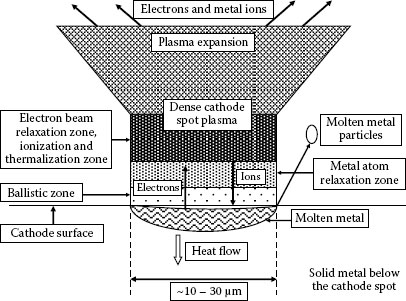
FIGURE 9.46
A model of the cathode spot showing its complexity (not to scale) [20].

9.6.2    The Columnar Vacuum Arc

If the current at the instant of contact separation approaches approximately 15 kA, the bridge rupture leads to formation of a single, high-vapor-pressure arc column. This arc is a high pressure arc and is similar to the arc described in Section 9.5 (see Figure 9.47). The appearance of the high-current vacuum arc has been extensively studied [72,93,95,96]. It has been shown that, depending on the current level and contact spacing, the diffuse arc can also form an anode spot and a columnar arc before going diffuse again close to current zero. It is possible, however, to form a columnar arc (Figure 9.48) from the initial bridge arc which will stay columnar until just before current zero. At the highest currents, the electrode regions of this columnar column exhibit intense activity, with jets of material being ejected from the contact faces [72,95]. In spite of this severe contact activity, even this arc mode can sometimes return to the diffuse mode just before current zero. Figure 9.49 shows an example of an arc appearance diagram developed by Heberlein and Gorman for a vacuum arc between butt contacts [72].

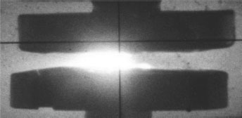
FIGURE 9.47
Photograph of a high-current vacuum arc.

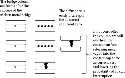
FIGURE 9.48
Possible modes of the vacuum arc appearance for high current vacuum arcs formed between opening contacts.

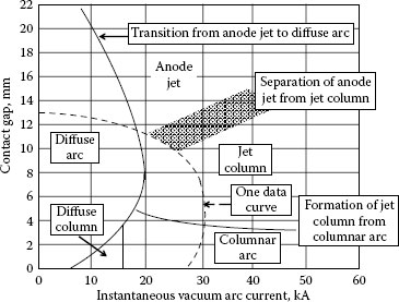
FIGURE 9.49
Vacuum arc appearance diagram for high-current vacuum arcs between butt contacts [72].

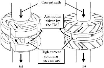
FIGURE 9.50
The motion of the high current columnar vacuum arc on transverse magnetic field contact structures, (a) spiral shaped contacts and (b) contrate cup-shaped contacts [20,94].

9.6.3    The Vacuum Arc in the Presence of a Transverse Magnetic Field

It is possible to prevent severe heating of the vacuum interrupter’s contact surfaces by subjecting the columnar arc to a transverse magnetic field and, thus, force the arc to rapidly travel around the perimeter of the contact. Figure 9.50 illustrates spiral and cup shaped contacts that have been successfully used to achieve this motion [20,94]. Schulman [95,96] has developed the appearance diagrams for high current arc motion between these spiral contacts.

9.6.4    The Vacuum Arc in the Presence of an Axial Magnetic Field

One method of creating a diffuse arc at high currents is to design a contact structure that applies an axial magnetic field [20,99], see for example Figure 9.51. For a sufficiently high axial field, the vacuum arc can be maintained in the diffuse mode to very high currents [97,98,99]. After the rupture of the molten metal bridge, a bridge column forms, and this arc slowly expands into a diffuse arc [99]. Once the arc has gone diffuse, the axial magnetic field forces the arc to remain diffuse. The electrons are confined by the magnetic field lines in the inter-contact region and, because of the associated creation of radial electric fields, the ions are also confined to the inter-contact region [20]. An example of a 10 kA diffuse arc is shown in Figure 9.52. During this high-current arcing the diffuse arc distributes the arc energy over the whole contact surface and thus prevents gross erosion of the contacts.

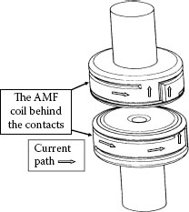
FIGURE 9.51
One contact design to force a high current vacuum arc into the diffuse mode as a result of an axial magnetic field structure behind the contact faces [20,94].

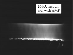
FIGURE 9.52
Photograph of a high-current (10 kA), diffuse vacuum arc formed with an axial magnetic field across the open contacts.

9.7    Arc Interruption

9.7.1    Arc Interruption in Alternating Current Circuits

A single phase ac circuit is shown in Figure 9.53. Here the ac power supply is connected to an inductive load by a cable and current is permitted to flow by closing the switch, S. Also shown is the circuit’s resistance and the inductor’s stray capacitance to ground. The analysis of the currents and voltages that occur when such a circuit is switched is beyond the scope of this book: it is the subject that requires a volume of its own [17,100]. It is enough for this section to use the example shown in Figure 9.54. Here the circuit has a large inductive component, i.e., the circuit current lags the system voltage. When the contacts in the switch open an arc is formed and burns to the first current zero. After the arc extinguishes at the natural ac current zero, the voltage across the contacts rises to about 1.7 times the circuit’s peak voltage in a few tens of microseconds to the line voltage and then exceeds it [17,20]. The voltage that appears across the contacts is called transient recovery voltage (TRV). Both the TRV and its rate of rise depend upon the circuit inductance and the stray capacitance in the circuit [20,100]. The process of arc interruption at current zero is of critical importance. The ac circuit reverses 2f/s where f is the power frequency. So in a 60 Hz circuit the current passes through a current zero 120 times each second (at 50 Hz it is 100 times each second). When the contacts part, the arc which forms allows the circuit current to flow to a natural current zero. As the current goes to zero, the energy input to the arc also goes to zero. For a brief time at current zero (I = 0) the energy lost by the arc and by the cathode and anode regions exceeds the energy input. This gives the gap between the contacts the opportunity to change from a reasonable electrical conductor to an insulator and thus prevent the continued flow of the current. If this occurs, the circuit is interrupted. All ac switches depend upon the arc to extinguish for the interruption of the current flowing in the circuit. It is important for the designers of these switches to understand the phenomena that occur at the contacts that cause the arc to extinguish.

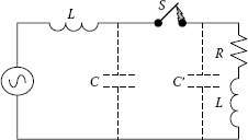
FIGURE 9.53
The alternating current ac circuit.

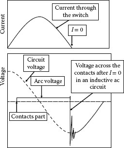
FIGURE 9.54
Interruption of an inductive ac circuit at current zero, showing the change in voltage across the open contacts.

Slepian [101] first described the arc extinction process in his “‘race theory,” where the recovery of the gap between the contacts depends upon two competing voltage values: (1) the TRV of the circuit, which is impressed across the contacts at current zero and is only dependent upon the circuit inductance, resistance, and capacitance, and (2) the increase in the dielectric strength of the residual arc channel. This is characterized by the voltage required to reignite the arc, called the reignition voltage. The reignition voltage increases with time. It is only dependent upon the contact gap parameters, such as the arc current before current zero, the gap length, contact material, arc chamber design, and the ambient gas, but it is independent of the circuit parameters. No dielectric breakdown and reignition of the arc can occur if the TRV across the contacts is below the reignition curve of the contact gap. Two empirical reignition curves are shown in Figure 9.55 [102,103]. The full reignition curve has the four distinct stages illustrated in Figure 9.56 [104].

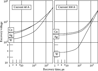
FIGURE 9.55
Recovery of Cu, Ag, and W contacts, with a 2 mm contact gap, after one ac half-cycle of arcing at 40 A and 300 A [102,103].

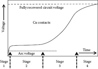
FIGURE 9.56
The four stages of recovery, an illustration of the free recovery/reignition characteristic.

1.  instantaneous recovery that occurs in <1 μs;

2.  a slight increase in the dielectric strength followed by a plateau;

3.  a steady increase in recovery that lasts between a few tens or a few hundred microseconds;

4.  the full dielectric strength of the “cold” contact gap.

This recovery process takes place in three stages.

•  Stage 1. The rapid adjustment of the plasma at I = 0 and the cessation of electron emission from the cathode.

•  Stage 2. The cooling of the arc column and the recombination of the ionized gas.

•  Stage 3. The long-term cooling of the whole arc chamber.

9.7.1.1    Stage 1 – Instantaneous Dielectric Recovery

Stage 1 is illustrated in Figure 9.57a and b. When the current reaches zero and the reverse voltage begins to appear across the contacts, the production of electrons at the old cathode stops. If no electrons emission is initiated at the new cathode, there will be a redistribution of the arc plasma close to the contact surfaces. First of all, during the initial recovery stage, the slow moving ions can be considered stationary, Figure 9.57a. As the TRV is applied across the open contacts (now with the reverse polarity) the electrons will be repelled instantaneously from the new cathode leaving a space charge sheath, Figure 9.57b. The cathode sheath is formed very close to the cathode approximately 10⁻⁷ m. The former arc column is a plasma, the 4th state of matter and thus must retain its charge neutrality, i.e., n_e = n_i. The electrons therefore must stay with stationary the ions. It has been shown experimentally that the space charge sheath reaches an instantaneous recovery voltage of about 300 V for a cold cathode. It is at this voltage the electric field at the cathode is high enough for electron emission to be initiated from the cold cathode: i.e., approximately 3 × 10⁹ V m⁻¹. If less than this instantaneous recovery voltage is impressed across the contact gap, all the voltage appears across the cathode sheath and none across the plasma column. If the voltage U_R appearing across the contact gap is greater than this instantaneous recovery voltage, then the voltage distribution shown in Figure 9.58 would occur. That is for a cold cathode, 300 V would appear across the cathode sheath and the voltage U_R – 300 V would be impressed on the plasma column. The value of the instantaneous recovery voltage does depend upon the condition of the new cathode’s surface as the recovery voltage is impressed across the open contacts. As Figure 9.55 shows this critical voltage is dependent upon the contact material and the level of current interrupted. The non thermionic emitting materials Cu and Ag have an instantaneous recovery voltage of about 300 V after interrupting currents of 40 and 300 A. In contrast, W, which is a thermionic emitter, has a much lower instantaneous recovery voltage after interrupting the 300 A arc. This can be expected, because the temperature of the new cathode would remain at a higher temperature after interrupting 300 A and the development of the cathode sheath. The new cathode would then be able to emit electrons thermionically with a much lower field. Thus, the voltage across the cathode sheath can be much lower. Figure 14.10 illustrates this how the value of the instantaneous recovery voltage changes for a number of contact materials as the circuit current interrupted increases from 25 to 1,300 A. The interesting aspect of these data is that instantaneous recovery voltage for the contact materials Ag-CdO (10 and 15 wt%), Ag-SnO₂(12 wt%) and Ag-Ni(10 wt%) is not greatly reduced for currents up to 1,300 A.

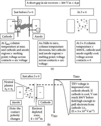
FIGURE 9.57
Stage 1: The initial rapid adjustment of the inter-contact plasma immediately after current zero in an ac circuit showing the development of the cathode sheath (not to scale) in front of the new cathode.

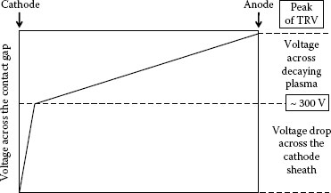
FIGURE 9.58
The voltage distribution across the contact gap (note the width of the cathode sheath is exaggerated).

Stage 1 is independent of contact gap as long as the gap is greater than that required for “vacuum breakdown.” It is, however, very dependent upon the properties of the contacts, e.g., melting and boiling point, thermal diffusivity, density, work function, ionization potential, and the dI/dt before I = 0. All effects that lower the probability of electron emission will increase the probability of arc extinction. If two sets of contacts are connected in series (e.g., a bridging contact structure) then instantaneous recovery voltage would be expected to double. Figure 14.11 shows that apart from Ag contacts value of the instantaneous recovery voltage is a little less than double for Ag–CdO (10 wt%), Ag–SnO₂ (12 wt%) and Ag–Ni (10 wt%) contacts.

9.7.1.2    Stage 2 – Decay of the Arc Plasma and Dielectric Reignition

Immediately after Stage 1 there is a comparatively slow increase in the dielectric strength of the contact gap. This is usually explained by axial heat conduction to the comparatively cool contact surfaces. Thus the gas temperature in these regions slowly decreases, the neutral gas density will increase and the ion density will decrease. The thickness of the cathode sheath during this stage also increases and thus reduces the electric field at the cathode and the probability of electron emission.

After this short time period of gas cooling near the contact surfaces and the extension of the cathode sheath, there is a gradual decay of the plasma conductance. Figure 9.59 gives an example of this for a 5 A and a 30 A arc [105]. As this figure shows even the middle of the plasma column is cooled down to a critical temperature where the thermal ionization according to Saha’s equation becomes negligible. In air at atmospheric pressure this critical temperature is on the range approximately 2,000–3,000 K [106]. At gas temperatures below this value the TRV will stress the whole gap between the contacts, i.e., the voltage is homogeneously distributed along the total contact gap and the breakdown voltage depends upon the gap length and the gas pressure or gas number density, n, which is proportional to (T⁻¹) as discussed in Section 9.3.

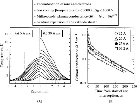
FIGURE 9.59
Stage 2: (A) Measured transient temperature profiles during free recovery for arcs in air of (a) 5 A: top curve shows the steady-state profile and the other curves show those after 20, 30, 50, 80, 105, 155, 200, 300, 500, 750, and 1,000 μs; (b) 30 A: top curve shows the steady-state profile and the other curves show those after 20, 50, 75, 100, 150, 200, 300, 500, 700, 750, and 1,000 μs. The upper steady-state curve in (a) corresponds closely with the profile at 100 us in (b) [74]. (B) Free conductance decay for arcs in air stabilized in a 0.5-cm-diameter tube for initial currents ranging from 12 to 36 A. For conductances of less than 0.2 Ω⁻¹ cm, the rate of decay for a given conductance is insensitive to the initial conditions [105,106].

The time it takes for the plasma column to cool depends strongly upon the design of the arc chamber. For example, it depends upon the contact gap; the shorter the contact gap the more effectively is the gas in the gap cooled by axial heat flow towards the “cool’ contact surfaces which act as heat sinks. Experimentally it has been shown that an optimum gap for the low current arcs (~<30 A) appears to be approximately 0.5 mm. It also depends upon the ionization potential of the ambient gas and is affected by impurities such as residual metal vapor. Some arc chambers have a magnetic drive to lengthen the column and perhaps to drive the arc into metal plates such as deion plates [107], which enhance the recovery effect (see Chapter 14 Sections 14.1.1 and 14.1.2). In high-voltage circuit breakers the cooling of the arc column is of paramount importance because in these devices the TRV exceeds the 300 V in a few microseconds after I = 0 [17]. A breakdown of the contact gap after a current pause at current zero and the appearance of the TRV across the contact gap is called a dielectric reignition.

9.7.1.3    Thermal Reignition

The voltage drop across the space charge sheath of approximately 300 V that forms in front of the cathode produces a field in front of the cathode that permits the field emission of electrons. If the TRV has a voltage greater than 300 V then the excess voltage appears across the decaying plasma, see Figure 9.58. Under the correct conditions, the electrons liberated from the new cathode by field emission can be accelerated by the voltage drop across the plasma and may cause the arc column to heat up again. This phenomenon is called thermionic reignition. If this happens a post-arc current can be sustained which might be able to heat up the arc column again. Thermal reignition is not decided by a race between two independent voltage curves as it is for dielectric reignition, but by a race between the electrical power input into the cooling arc column and the rate of energy loss by the arc column. The electrical power input is controlled by the supply voltage, the circuit impedance and the continuous change in the arc conductance (see Figure 9.59). The rate of energy loss by the arc column depends upon the ambient gas, the contact gap and the whole design of the arc chamber.

A more extreme case of reignition occurs if the new cathode is able to emit electrons right after I = 0 and the instantaneous formation of the insulating positive space charge layer in front of the cathode is limited or is prevented. This is called thermal reignition. Electron emission will occur most easily if the old anode (or new cathode) is very hot just before I = 0 and electrons are thermionically emitted, e.g., a recovering arc between refractory contacts (C, W, Mo) or the contacts are covered by a refractory surface layer, e.g., oxides of Mg, Al, Mn, Mo. Compare the recovery curves at 40 and 300 A for tungsten contacts in Figure 9.55. An excellent example of an arc chamber specifically designed for reignition of the electric arc at current zero is a high-pressure sodium street lamp [108]. Here the electrodes are made from tungsten coils in which is deposited a Thoria paste to ensure the emission of copious electrons at each I = 0. In this case the thermionic electron emission certainly prevents the initial recovery process (Stage 1). Thermionic reignition will occur, however, even with non-refractory contact materials if the arc root has caused gross melting at the anode and the voltage across the cathode sheath is enough to initiate T–F electron production (see Section 9.5.2). Thermal reignition and thermionic reignition can occur between non-refractory contacts that try to interrupt currents greater than a few hundred amperes in medium voltage circuits unless measures are taken to rapidly cool the arc column.

Simplified power balance equations were formulated by Cassie [109] and Mayr [110] and later improved by Frost and Browne [111]. Much of the design of high current switching devices used in circuits where the voltage is greater than 300 V is dependent upon optimizing the rate of decay of the residual arc plasma after I = 0 [17] (see also Chapter 14).

9.7.2    Arc Interruption in Direct Current Circuits

The arc interruption process follows the same physical principles as has already been discussed for ac circuits (see Section 9.7.1). The major difference is that a dc switch has to develop its own current zero before electron emission at the cathode ceases and the space charge sheath can develop. If we take a typical dc circuit (Figure 9.60),

$U_{\text{C}}=L\frac{\text{d}I}{\text{d}t}+RI+U_{\text{A}}$

(9.52)

where U_C is the voltage of the dc power supply, L is the circuit inductance, R is the circuit resistance, I is the current and U_A is the arc voltage across the opening contacts. Rearranging Equation 9.52,

$\frac{\text{d}I}{\text{d}t}=\frac{1}{L}\left(\left[U_{\text{C}}-RI\right]-U_{\text{A}}\right)$

(9.53)

Before the contacts begin to open U_C = RI and U_A equals zero, so dI/dt = 0. As soon as the arc is initiated at t = 0, dI/dt must have a negative value equal to −U_A/L, i.e., the current initially decreases. If the term (U_C − RI) at some point equals U_A, then di/dt again will equal zero and the current will cease decreasing. This is a stable point and in the circuit shown in Figure 9.61, a stable arc will exist. The basic criterion for arc interruption, therefore, is that U_A must at least equal (U_C – RI). Figure 9.61 shows two examples of voltage–current arc characteristics: (see Section 9.5.5) (1) U_ARC1 intersects U_C – RI and the arc in this condition is stable at the lower value where the curves intersect; (2) A characteristic like U_ARC2 would always ensure arc interruption.

For dc interruption not only must you establish the arc once the contacts part, but you must also ensure that the arc voltage is forced to reach the system voltage. This will ensure that the current flowing in the circuit is forced to zero and the contact gap recovery processes can be established. The arc voltage can be increased by lengthening the arc, or by cooling it is a number of ways, see Chapters 13 and 14. The recovery process follows the same stages as have been discussed for ac current interruption. Figure 9.63 is an example of AgCdO contacts interrupting an 8 A, 63 V dc circuit [112]. Using this figure and Figure 9.62 the interruption of this circuit can easily be explained. It can be seen in Figure 9.62 that once the arc forms after the rupture of the molten metal bridge the minimum arc voltage of ~12.9 V appears across the opening contacts. This results in a sudden drop in the circuit current to ~6.36 A. A momentary stable point on the voltage/current characteristic, U_ARC1, in Figure 9.63 is established As the contacts continue to open the arc lengthens, the arc voltage U_ARC increases as a result of the arc column lengthening and the transition from a metal phase arc to an arc in the ambient gas, air (see Section 10.3.5). After 2 ms the contacts in Figure 9.62 have opened to 1 mm and U_ARC2 ≈ 24.7 V. Now the current has decreased to ~ 4.86 A. A new momentary stable point is now established in Figure 9.63 on the voltage/current characteristic that reflects the higher contact gap and the decrease in current. Incidentally this is what you might have expected from Figure 9.39. At 4 ms the contacts have opened to 2 mm and the arc voltage U_ARC3 ≈ 42 V and the current has now decreased to ~ 2.7 A. Thus, another new momentary stable point is established in Figure 9.63 that results from the increased arc length and the lower current. I might be expected that this process would continue until U_ARC4 + RI ≈ U_C as shown in Figure 9.63. However, as can be seen in Figure 9.62, at a contact spacing of 2.2 mm when the current has decreased to ~ 2.2 A the current begins to decrease rapidly. Here the energy supplied to the arc (U_A × I_C) can no longer make up for the energy lost by the arc. The −dI/dt increase rapidly with rapid increase with dU_ARC/dt and the circuit is interrupted. The small current trapped in the circuit inductance results in a small spike in the voltage across the contacts before the open circuit voltage of ~63 V appears across them. It is important to note that when observing this opening process in dc circuits that the I_min is quite different from that discussed in Section 9.5.4. It has a much higher value. The reason for this is (1) the arc shown in Figure 9.62 is operating in air and not in metal vapor and (2) as the arc becomes longer the energy to sustain it must be at least equal to the energy losses from the increased arc length and may also include energy loss by radiation. Thus, I would expect that when interrupting higher voltage circuits where longer arc lengths would be required, the I_min would be even higher than in 2.7 A shown in Figure 9.62.

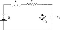
FIGURE 9.60
The direct current dc circuit.

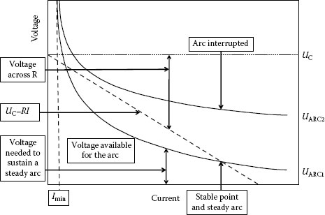
FIGURE 9.61
The conditions for a stable arc and for interruption of a dc circuit (arbitrary scales for voltage and current).

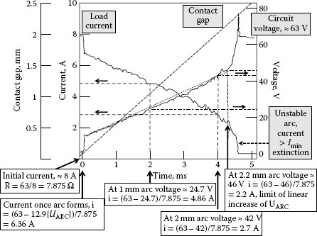
FIGURE 9.62
The voltage and current for AgCdO contacts opening at 0.5 m.s⁻¹ and interrupting a 8 A, 60 V dc mostly resistive circuit [112].

Once the current zero has been established, the interruption process is shown in Figure 9.64a and b. The sequence is similar to that discussed for ac interruption. The major difference being the cathode remains the cathode and the anode remains the anode. Stage 1 is illustrated in Figure 9.64a and b. Stages 2–4 are similar to those discussed for ac current interruption.

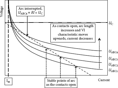
FIGURE 9.63
Illustration of dc circuit interruption for use with Figure 9.62 (arbitrary scales for voltage and current).

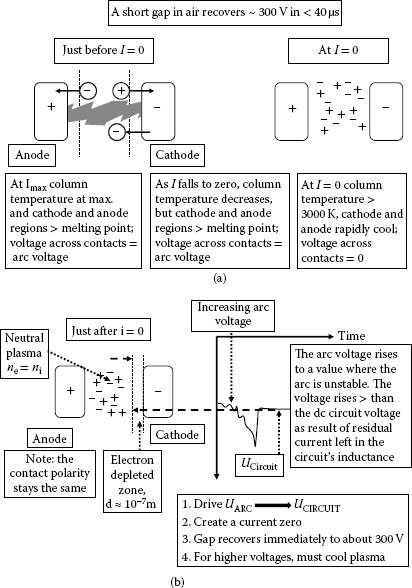
FIGURE 9.64
Stage 1: The initial rapid adjustment of the inter-contact plasma immediately after the forced current zero in a dc circuit showing the development of the cathode sheath (not to scale) in front of the cathode.

9.7.3    Vacuum Arc Interruption in Alternating Circuits

All successful vacuum interrupter designs have contacts that force the vacuum arc to go diffuse before the current reaches zero [20,94]. At current zero, the vapor-producing cathode spots extinguish. The residual vapor and plasma within the inter-contact region rapidly condense and recombine on both the shield and contact surfaces, and the original vacuum condition is rapidly approached. Analysis of the recovery processes directly following current zero is complicated by the non-uniform distribution of the reapplied voltage in the recovering arc gap. In the presence of residual plasma, the circuit voltage is impressed across a narrow space-charge sheath at the new cathode [20,113,114]. The ac circuit is successfully interrupted if the instantaneous dielectric strength of the recovering inter-contact gap always exceeds the circuit reapplied voltage. Full recovery can be attained within microseconds of current zero. This ultimate breakdown voltage depends on both the spacing and geometry of the internal shields, and also on the electric field stress on the external envelope of the interrupter. Further, the ultimate breakdown voltage is critically dependent on the spacing of the contacts, the condition of the arced contact surfaces, and the magnitude and duration of the recovery voltage [20].

The presence of stationary anode spots during the arcing half cycle can adversely affect dielectric recovery due to (1) associated increases in the inter-contact plasma and vapor densities, (2) continued evaporation from the localized hot spot following current zero, and (3) for the case of refractory materials such as carbon and tungsten, continued thermionic emission of electrons following contact polarity reversal [20].

9.7.4    Arc interruption of Alternating Circuits: Current Limiting

The technique used for dc circuit interruption can also be employed in ac circuits to limit the magnitude and the duration of the current that occurs when a circuit breaker is operating to interrupt a short circuit fault current. Molded case circuit breakers that are used to protect a wide range of circuits, from household circuits (110 to 240 V rms) to industrial distribution circuits (up to 600 V rms), are increasingly using a current limiting technique [115,116]: see also Chapter 14. As soon as a fault current is initiated, the circuit breaker’s contacts open very quickly and an arc is formed. The arc voltage is then driven to a high value, greater than the ac circuit voltage, by stretching it and forcing it into metal plates: see Chapter 14. Figure 9.65 illustrates the effect for a symmetrical resistive ac circuit and for an asymmetrical inductive ac circuit. Once the arc voltage is greater than the circuit’s system voltage the current is limited and rapidly goes to zero, where the arc extinguished and the circuit is interrupted. How quickly the arc voltage rises depends upon the sensing of the fault current, the contact opening speed and the design of the arc chamber. Even gassing from the arc chamber walls can greatly influence the voltage rise [117]. Any gap in the arc runners can also affect the speed of the arc’s motion [118]. Many circuit breaker designs now use the principle of dc interruption (i.e., of driving the arc voltage above the circuit voltage) in ac circuits to create a new current zero. In doing so the fault current is greatly reduced both in magnitude and duration.

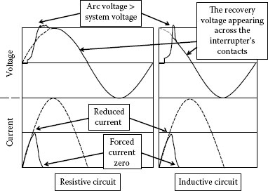
FIGURE 9.65
Illustration of current limiting in resistive and inductive ac circuits.

9.7.5    Interruption of Low Frequency and High Frequency Power Circuits

Most electrical ac power generation systems have a frequency of 50 or 60 Hz. This depends upon a country’s historical development of its electrical grid. There are some systems, however, that use lower frequencies. Some electric locomotive systems use 16 2/3 Hz and others 25 Hz. Higher frequencies up to 400 Hz are used for electric ship development. When such circuits install a circuit breaker designed to protect 50/60 Hz circuits, the question arises, “How well will they perform?” There is a dearth of published literature on this subject. One study [119] is shown in Figure 9.66. Here the fault current interrupting ability of a vacuum interrupter has been evaluated for frequencies from 16 2/3 to 800 Hz. It shows that the maximum performance is close to its design value at 80 Hz and that its performance drops as the frequency drops or increases. Thus a circuit breaker designed to protect a circuit at 50/60 Hz should be de-rated for use in circuits with lower or higher ac frequencies.

9.7.6    interruption of Megahertz and Gigahertz Electronic Circuits

The use of mechanical switches to control very high frequency circuits at first sight seems unusual. Solid state devices such as MOSFETS [120] have been successfully employed and have performed well for many decades. The main task of any switching device is to conduct the high frequency current when closed with a low insertion loss and, when open, to provide complete isolation. Table 9.10 [121] compares the MOSFET with three mechanical switches: (a) MEMS [122] (see Chapter 12), (b) a reed relay (see Chapter 11) and (c) an electro-mechanical relay. As the comparison shows the electro-magnetic relay has the lowest insertion loss (i.e. contact resistance) and the highest potential for circuit isolation (i.e. breakdown voltage). Johler [123] has shown indirect evidence of the switching ability of the electro-magnetic relay for frequencies over range from 0.8 to 3 GHz and power ranges from 1 to 37 W. Table 9.11 shows the time of a half cycle for ac frequencies from 50 Hz to 10 GHz.

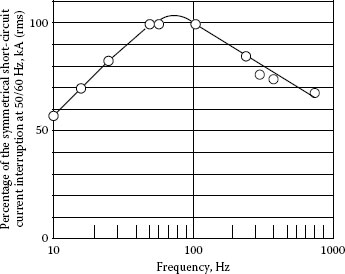
FIGURE 9.66
The interruption ability of a vacuum interrupter as a function of the electrical system’s frequency [117].

TABLE 9.10
Comparison of the Characteristics of Solid State and Mechanical Switches for Controlling High Frequency Circuits

TABLE 9.11
The Durations of One Half Cycle of Current for Frequencies from 50 Hz to 10 GHz

Frequency	Time 1/2-Cycle	Frequency	Time 1/2-Cycle
50/60 Hz	10/8.3 ms	500 kHz	1 μs
500 Hz	1 ms or 1,000 μs	1 GHz	0.5 μs or 500 ns
100 kHz	5 μs	10 GHz	50 ns

On closing an electro-magnetic relay would generally have some contact bouncing and may take up to 40 μs to finally close [123]. Thus for a 1 GHz current up to 40 cycles would pass through the switch from the initial contact touch until the contacts would be completely closed. Miki et al. [124,125] have shown that the interruption of high frequency currents in up to 800 MHz does rely upon the existence of their current zero occurring every half cycle. Figure 9.67 shows a typical opening at about 0.5 ms⁻¹ for a 500 Hz current in a mostly resistive 2 A circuit with a circuit voltage of 40 V (peak). Once the contacts part and the metallic arc is established it operates with a U_min between 10 and 15 V. The arc remains stable until the current drops below I_min (between 0.3 and 0.5 A) when in becomes unstable and chops out. A recovery voltage which is characteristic of the stray inductance and capacitance of the circuit reaches a peak value of about 60 V. In this example the arc is stable for about 0.5 μs so the contact gap when the arc is interrupted is about 0.25 μm. In this case the gap is sufficient to hold off the recovery voltage. Miki et al. show that interruption of circuits with frequencies less than or equal to 500 kHz always interrupt at the first current zero if the arcing time is greater than 1/4 cycle. Above 500 kHz the arc is not interrupted at the first current zero. Figure 9.68 illustrates this for a 1 MHz circuit. The contact gap at the first current zero after 0.28 μs of arcing is about 0.14 μm, which is insufficient to hold off the recovery voltage. The researchers show that for frequencies above 500 kHz in their circuit about 2 μs of arcing is needed or a contact gap of about 1 μm is required before the circuits are completely interrupted. Johler [121] also finds that making or breaking higher frequency RF loads (up to 3 GHz) requires the arc to operate over several periods of the current before interruption is achieved. Again the contact gap must achieve a minimum value before the recovery voltage can be withstood. These data show that interruption of very high frequency currents is possible using electrical contacts. Thus the advantage of the low insertion impedance and the high isolation is attainable as long as the longer interruption and the longer switch-on times are acceptable.

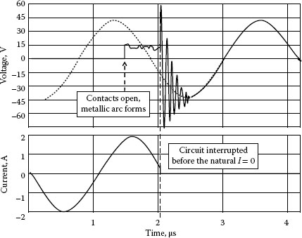
FIGURE 9.67
Arc behavior and interruption of a 2 A, 40 V (peak), 500 kHz circuit [124,125].

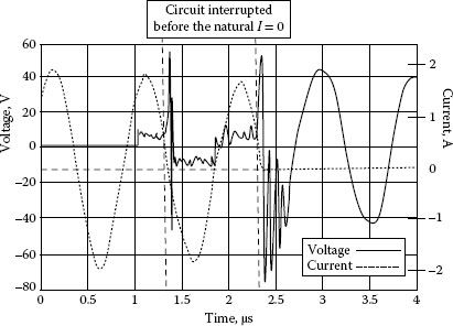
FIGURE 9.68
Arc behavior, reignition and interruption of a 2 A, 40 V (peak), 1 MHz circuit [124,125].

Acknowledgments

I am extremely grateful to the late Professor Werner Rieder for his critical review of the initial version of this chapter, his attention to scientific detail, his many suggestions for changes, and his encouragement. All of which have improved the substance and breadth of the chapter. I also appreciate the use of the photographs taken by Erik Taylor (Figures 9.45, 9.47, and 9.52).

REFERENCES

1.  JM Meek, JD Craggs. Electrical Breakdown of Gases. Oxford: Clarendon Press, 1953.

2.  For the reader who wishes to pursue further the kinetic theory of gases, a good place to begin is a good University level Physics text such as: G Joos and I Freeman. Theoretical Physics. 3rd edition. London: Blackie, Part VI, pp 563–598, 1960.

3.  H Davy. Elements of Chemical Philosophy, Vol. 1. London: Smith and Elder, 1812, p. 152.

4.  JJ Thompson. On the cathode rays. Proc. Cambridge Phil. Soc 10: 74, 1899.

5.  N Bohr. The Theory of Spectra and Atomic Constitution. Cambridge: Cambridge University Press, 1922.

6.  JS Townsend. Electricity in Gases. Oxford: Clarendon Press, 1915.

7.  A von Engel. Ionized Gases. Oxford: Clarendon Press, 1955.

8.  W Elenbaas. The High Pressure Mercury Vapor Discharge. Amsterdam: North-Holland, 1951.

9.  W Finkelnburg, H Maecker. Elektrische Bogen und thermische Plasmen. In: S Fluegge, ed. Handbuch der Physik, Vol. 22. Berlin: Springer-Verlag, 1956.

10.  JM Sommerville. The Electric Arc. London: Methuen, 1959.

11.  JD Cobine. Gaseous Conductors. New York: Dover, 1958.

12.  TH Lee. Physics and Engineering of High Power Switching Devices. Cambridge, MA: MIT Press, 1975.

13.  HN Wagar. Contact and connection technology. In: D Baker, D Koehler, W Fleckenstein, C Roden and R Sabia, eds. Integrated Device and Connection Technology, Vol. III. Englewood Cliffs, NJ: Prentice Hall, 1971.

14.  R Holm, E Holm. Electric Contacts: Theory and Application. New York: Springer-Verlag. 3rd Printing, 2000.

15.  JM Lafferty, ed. Vacuum Arcs, Theory and Applications. New York: Wiley-Interscience, 1980.

16.  MF Hoyaux. Arc Physics. New York: Springer-Verlag, 1968.

17.  TE Browne. Circuit Interruption, Theory and Techniques. New York and Basel: Marcel Dekker, 1984.

18.  F Llewellyn-Jones. Ionization and Breakdown in Gases, London: Methuen/New York: Wiley, 1957.

19.  F Paschen. Über die zum Funkenübergang in Luft, Wasserstoff, und Kohlensäuer bei verschiedenen Drucken erforderliche Potentialdifferenz. Wied Ann 37(3): 69–96, 1889.

20.  PG Slade. The Vacuum Interrupter, Theory, Design and Application, Boca Raton, FL: CRC Press, 2008.

21.  RV Latham. High Voltage Vacuum Insulation. London: Academic Press, 1995.

22.   RR Fowler, LW Nordheim. Electron emission in intense electric fields. Proc. R. Soc. A119: 173–181, 1928.

23.  PG Slade, ED Taylor. Electrical breakdown in atmospheric air between closely spaced (0.2 μm–40 μm) electrical contacts, IEEE Trans. Compon. Pack. Tech. 25: 390–396, 2002.

24.  WB Maier, A Kadish, CJ Buchenauer, RT Robiscoe. Electrical discharge initiation and a microscopic model for formative time lags. IEEE Trans. Plasma Sci. 21(6): 676–683, 1993.

25.  N Wakatsuki, H Homma. Melting phenomena and arc ignition of breaking relay contacts, Proceedings of the 54th IEEE Holm Conference on Electrical Contacts: 15–20, 2008.

26.  T Utsumi. Theoretical and experimental investigations of the dynamic molten bridge. IEEE Trans. Parts Mater. Pack. PMP 5(1): 62–68, 1969.

27.  K Miyajima, S Nitta, A Mutoh. A proposal on contact surface model of electro-magnetic relays—based on the change of showering arc wave formations with the number of contact operations. IEICE Trans. Electron. E81-C(3): 399–407, 1998.

28.  H Ishida, Y Watanabe, M Taniguchi, H Inoue, T Takago. Observation of contact bridge phenomena at transient and steady state. Proceedings of the 50th IEEE Holm Conference on Electrical Contacts: 519–522, 2004.

29.  JW McBride, L Jiang, C Chianrabutra. Fine transfer in electrical switching contacts using gold coated carbon nano-tubes. Proceedings of the 26th International Conference on Electrical Contact Phenomena: 353–358, 2012.

30.  PG Slade, MD Nahemow. Initial separation of electrical contacts carrying high currents. J. Appl. Phys. 42(9): 3290–3297, 1971.

31.  PP Koren, MD Nahemow, PG Slade. The molten metal bridge state of opening electric contacts. IEEE Trans. Parts Hyb. Pack. PHP–11(1): 4–10, 1975.

32.  PG Slade, MF Hoyaux. The effect of electrode material on the initial expansion of an arc in vacuum. IEEE Trans. Parts Hyb. Pack. PHP–8: 35–47, 1972.

33.  PG Slade. The transition from the molten metal bridge to the metallic phase bridge column arc between electrical contacts opening in vacuum, Proceedings of the 23rd International Symposium on Discharges and Electrical Insulation in Vacuum, 198–201, 2008.

34.  R Haug, T Kouakou, J Dorémieux. Phenomena proceeding arc ignition between opening contacts: experimental study and theoretical approach. Proceedings of the 36th IEEE Holm Conference on Electrical Contacts: 543–549, 1990.

35.  M. Hopkins, R. Jones, J. Evans. Short time transients in electrical contacts. Proceedings of the 8th International Conference on Electrical Contacts: 270–272, 1976.

36.  PG Slade. Opening contacts: the transition from the molten metal bridge to the electric arc, IEICE Trans. Electron. E93-C(6): 1380–1386, 2010.

37.  PG Slade, The transition to the metal phase arc after the rupture of the molten metal bridge for contacts opening in air and vacuum. Proceedings of the 54th IEEE Holm Conference on Electrical Contacts: 1–8, 2008.

38.  V Puchkarev, M. Bochkarev. High current density spotless vacuum arc as a glow discharge. IEEE Trans. Plasma Sci. 25(4): 593–597, 1997.

39.  W. Ebling, A. Foster, R. Radtke, Physics of Non-Idealized Plasmas. Stuttgart: Teubner Verlagsgesell-schaft, 1991.

40.  L Holtgreven. Plasma Diagnostics. New York: Wiley Interscience, 1968.

41.  PG Slade, E Schulz-Gulde. Spectroscopic analysis of high-current, free-burning ac arcs between copper contacts in argon and air. J. Appl. Phys. 44(1): 157–162, 1973.

42.  MN Saha. Ionization in solar chromosphere. Philos. Mag. 40: 472, 1920.

43.  CG Suits. The temperature of the copper arc. Proc. NAS, Phys. 21(1): 48–50, 1935.

44.  JVR Heberlein, CW Kimblin, A Lee. Nature of the electric arc. In: TE Browne, ed. Circuit Interruption, Theory and Technique, New York: Marcel Dekker, 1984, pp. 135–157.

45.  W. Elenbaas. Ähnlichkeitsgesetze der Hochdruckentladung.: Physica 2, p. 169, 1935.

46.  G Heller. Dynamic similarity laws of the mercury high pressure discharge. Physics. 6: 389, 1935.

47.  JJ Lowke. Calculated properties of vertical arcs stabilized by natural convection. J. Appl. Phys. 50(1): 147–157, 1979.

48.   JJ Lowke. Simple theory of free burning arcs. J. Phys. D Appl. Phys. 12: 1873–1885, 1979.

49.  X Zhou, L Qi, B Liu, G Zhai. Study on static arc behavior in a relay considering influence of the silver alloy. Proceedings of the 26th International Conference on Electrical Contact Phenomena: 353–358, 2012.

50.  AE Guile. Arc-Electrode phenomena. Proc. IEEE (Lond.) IEEE Rev. 118(9R): 1131–1154, 1971.

51.  X Zhou, J Heberlein, E Pfender. Theoretical study of factors influencing arc erosion of cathode. Proceedings of the 38th IEEE Holm Conference on Electrical Contacts: 71–78, 1992.

52.  IG Kesaev. Cathode Processes in the Mercury Arc. Moscow: State Power Engineering Press, 1961 (translated and published in English by Consultants Bureau, New York, 1964).

53.  TH Lee, A Greenwood. Theory for the cathode mechanism in metal vapor arcs. J. Appl. Phys. 32: 916–923, 1961.

54.  C Spatami, D Teillet-Billy, JP Gauyacq, Ph Teste, JP Chabrier. Ion assist emission from a cathode in an electric arc, J. Phys. D Appl. Phys. 30: 1135–1145, 1997.

55.  JD Cobine. Introduction to vacuum arcs. In: JM Lafferty, ed. Vacuum Arcs Theory and Application. New York: Wiley-Interscience, 1980, pp. 8–12.

56.  J Heberlein, J Mentel, E Pfender. The anode region of electric arcs: a survey. J. Phys. D Appl. Phys. 43: 1–31, 2010.

57.  N Ben Jemaa, JL Queffelec, D Travers. Theoretical multisite arc model applied to statistical arc duration measurement on low break at low electrical level. Proceedings of the 30th Holm Conference on Electrical Contacts: 573–579, 1984.

58.  N Ben Jemaa, L Lehfaoui, L Nedelec. Short arc duration at low current (<1 A) and voltage (14–42 Vdc), Proceedings of the International. Conference on Electrical Contacts: 379–384, 2000.

59.  N Ben Jemaa. Short arc duration laws and distributions at low current (<1 A) and voltage (14–42 Vdc). IEEE Trans. Compon. Packaging Technol. 24(3): 358–363, 2001.

60.  N Ben Jemaa. Contacts conduction and switching in dc levels, Proceedings of the 48th IEEE Holm Conference on Electrical Contacts: 1–15, 2002.

61.  M Hasegawa, Y Kamada. An experimental study on re-interpretation of minimum arc current of electrical contacts. IEICE Trans. Electron. E88–C(8): 1616–1619, 2005.

62.  M Hasegawa, Y Tamaki, Y Kamada. An experimental study of minimum arc current of relay contacts and possible re-interpretation of the meaning thereof. Proceedings of the 52nd IEEE Holm Conference on Electrical Contacts: 153–158, 2006.

63.  M Hasegawa. An experimental study of minimum arc current of Ag contacts with different opening speeds. Proceedings of the. 53rd IEEE Holm Conference on Electrical Contacts: 294–299, 2007.

64.  K Suhara. Arc extinction and reignition at a fixed short gap—a research on arc V-I characteristics. IEICE Trans. Electron. E87–C(8): 1348–1355, 2004.

65.  W Reider, H Schneider. Ein Beitrag zur Physik des Gleichstromlichtbogens. Elin-Z 5: 174–187, 1953.

66.  JW McBride, SM Sharkh. The influence of contact opening velocity on arc characteristics. Proceedings of the 16th International Conference on Electrical Contacts: 395–400, September 1992.

67.  J Sekikawa, T Kubono. An experimental equation of V-I characteristics of breaking arc for Ag, Au, Cu and Ni electrical contacts. IEICE Trans. Electron. E86-C(6): 926–931, 2003.

68.  W Reider. Leistungsbilanz der Electroden und Charakteristiken frei brennender Bogen. Z Physik. 146: 629–643, 1956.

69.  LA King. The voltage gradient of the free burning arc in air or nitrogen. Proceedings of the 5th International Conference on Ion Phenomena in Gases: 871, 1961.

70.  GR Jones, GH Freeman, H Edels. Transient temperature distributions in cylindrical arc columns following abrupt current changes. J. Phys. D Appl. Phys. 4: 236–245, 1971.

71.  RG Colclaser. Electrical and system aspects. In: TE Browne, ed. Circuit Interruption: Theory and Techniques. New York: Marcel Dekker, 1984, pp. 11–38.

72.  JVR Heberlein, JG Gorman. The high current metal vapor arc column between separating electrodes. IEEE Trans. Plasma Sci. PS–8, 283–289, 1980.

73.   MB Schulman, PG Slade. Sequential modes of drawn vacuum arcs between butt contacts for currents in the range 1 kA to 16 kA. IEEE Trans. Compon. Packaging Manuf. Tech. 18(1): 417–422, 1995.

74.  BE Djakov, R Holmes. Cathode spot division in vacuum arcs with solid metal cathodes. J. Phys. D Appl. Phys. 4: 504–509, 1971.

75.  LP Harris. Arc cathode phenomena. In: JM Lafferty, ed. Vacuum Arcs: Theory and Application. New York: Wiley, 1980, pp. 120–168.

76.  B Juttner. Formation time and heating mechanism of arc cathode craters in vacuum. J. Phys. D Appl. Phys. 14: 1265–1275, 1981.

77.  JE Daalder. Cathode-Erosion of Metal Vapor Arcs in Vacuum. Thesis, University of Eindhoven, The Netherlands, 1978.

78.  CW Kimblin. Erosion and ionization in the cathode spot regions of vacuum arcs. J. Appl. Phys. 44: 3074–3081, 1973.

79.  E Hantzsche. Theories of cathode spots. In: RL Boxman, PJ Martin and DM Sanders, eds. Handbook of Vacuum Arc Science and Technology. New Jersey: Noyes, 1995, pp. 151–208.

80.  I. Beilis. Theoretical Modeling of Cathode Spot Phenomena. In: RL Boxman, PJ Martin and DM Sanders, eds. Handbook of Vacuum Arc Science and Technology. New Jersey: Noyes, 1995, pp. 151–256.

81.  JE Daalder. Erosion and the origin of charged and neutral species in vacuum arcs. J. Phys. D Appl. Phys. 8: 1647–1659, 1975.

82.  DT Tuma, CL Chen, DK Davies. Erosion products from the cathode spot region of a copper vacuum arc. J. Appl. Phys. 49: 3821–3821, 1978.

83.  Z Zalucki, J Kutzner. Ion currents in the Vacuum arc. Proceedings of the 8th International Symposium Discharges Electrical Insulation Vacuum, August 1976, pp. 297–302.

84.  JVR Heberlein, DR Porto. The interaction of vacuum arc ion currents with axial magnetic fields. IEEE Trans Plasma Sci. PS–11: 152–159, 1983.

85.  CW Kimblin. Vacuum arc ion currents and electrode phenomena. Proc. IEEE. 59: 546–555, 1971.

86.  WD Davies, HC Miller. Analysis of the electrode products emitted by dc arcs in a vacuum ambient. J. Appl. Phys. 40: 2212–2221, 1969.

87.  AA Plyutto, VN Ryzhkov, AT Kapin. High speed plasma streams in vacuum arcs. Sov. Phys. JETP (New York) 20: 328–337, 1965.

88.  LP Harris. A mathematical model for cathode spot operation. Proceedings of the 8th International Symposium Discharges Electrical Insulation in Vacuum, 1978, pp. F1–F18.

89.  G Yushkov, A Bugaev, I Krinberg, E Oks, On a mechanism of ion acceleration in vacuum arc-discharge plasma. Doklady Phys. 46(5): 307–309, 2001.

90.  E Byon, A Anders, Ion energy distribution functions of vacuum arc plasmas. J. Appl. Phys. 93(4): 1899–1906, 2003.

91.  HC Miller. A review of anode phenomena in vacuum arcs. Contrib. Plasma Phys. 29(3): 223–249, 1989.

92.  CW Kimblin. Anode voltage drop and anode spot formation in vacuum arcs. J. Appl. Phys. 40: 1744–1752, 1969.

93.  GR Mitchell. High current vacuum arcs: Part I and II. Proc. IEEE (London). 177: 2315–2332, 1970.

94.  PG Slade. The vacuum interrupter contact. IEEE Trans. Compon. Packaging Manuf. Tech. 7(1): 25–32, 1984.

95.  MB Schulman. Separation of spiral contacts and the motion of vacuum arcs at high AC currents. IEEE Trans. Plasma Sci. 21(5): 484–488, 1993.

96.  MB Schulman. The behaviour of vacuum arcs between spiral contacts with small gaps. IEEE Trans. Plasma Sci. 23(6): 915–918, 1995.

97.  CW Kimblin, RE Voshall. Interruption ability of vacuum interrupters subjected to axial magnetic fields. Proc. IEEE (London). 119: 1754–1758, 1972.

98.  S Yanabu, S Souma, T Tamagawa, S Tamashita, T Tsutsumi. Vacuum arc under an axial magnetic field and its interrupting ability. Proc. IEEE (London). 126(4): 313–320, 1979.

99.   MB Schulman, PG Slade, JVR Heberlein. Effect of an axial magnetic field upon the development of the vacuum arc between opening electric contacts. IEEE Trans. Compon. Hyb. Manuf. Tech. 16(1): 180–189, 1993.

100.  A Greenwood. Electrical Transients in Power Systems, 2nd edition. New York: Wiley, 1991.

101.  J Slepian. Extinction of an a-c Arc. AIEE Trans. 47: 1398–1408, 1928.

102.  HA Bentounes. Influence de la nature des electrodes sur la vitesse de retablissement de la rigidite dielectrique d’un milieu post-arc. Thesis Universite de Paris-Sud Centre d’Orsay, No 651, 1984.

103.  HA Bentounes, J Muniesa. Electrode materials and recovery of the post-arc dielectric strength. Proceedings of the 13th International Conference on Electrical Contacts: 176–180, September 1986.

104.  H Edels and FW Crawford. Arc interruption. J. IEE. 2: 712–716, 1956; 3: 88–93, 1957.

105.  CW Kimblin, JJ Lowke. Decay and thermal reignition of low-current cylindrical arcs. J. Appl. Phys. 44(10): 4545–4547, 1973.

106.  FW Crawford, H Edels. The reignition voltage characteristics of freely recovering arc. Proc. IEEE. 107A: 202–212, 1960.

107.  A Lee, PG Slade. Molded-case, low-voltage circuit breakers. In TE Browne, ed. Circuit Interruption, Theory and Techniques, New York: Marcel Dekker, 1984, pp. 527–565.

108.  JF Waymouth. Electric Discharge Lamps. Cambridge, MA: MIT Press, 1971.

109.  AM Cassie. Arc Rupture and Circuit Severity: A New Theory. CIGRE. Report 102, Paris, 1939.

110.  O Mayr. Beitrage zur Theorie des statischen und des dynamischen Lichtbogens, Arc Elektrotech. 37: 588–608, 1943.

111.  LS Frost, TE Browne. Calculation of arc-circuit interaction. In TE Browne, ed. Circuit Interruption, Theory and Techniques, New York: Marcel Dekker, 1984, pp 187–240.

112.  SMS Sharkh, J McBride. Voltage steps in atmospheric low current arcs between opening silver metal oxide contacts. Proceedings of the 43rd IEEE Holm Conference on Electrical Contacts: pp. 233–237, 1997.

113.  M Glinkowski and A Greenwood. A computer simulation of post-arc plasma behaviour at short contact separation in vacuum. IEEE Trans. Plasma Sci. 17: 45–50, 1989.

114.  B Fenski, M Lindmayer. Post arc currents of vacuum interrupters with radial and axial magnetic field contacts – measurements and simulations. Proceedings of the 19th International Conference on Electrical Contact Phenomena, pub. VDE: 259–267, 1998.

115.  A. Lee, PG Slade. Molded-case, low-voltage circuit breakers. In TE Browne, ed. Circuit Interruption, Theory and Techniques. New York and Basel: Marcel Dekker, Chapter 14, 1984, pp. 155–561.

116.  D Chen, H Liu, H Sun, Q Liu, J Zhang. Effect of magnetic field of arc chamber and operating mechanism on current limiting. IEICE Trans. Electron. E86-C, 6: 915–920, 2003.

117.  C Rümpler, H Stammberger, A Zacharias. Low-voltage arc simulation with out-gassing polymers. Proceedings of the 57th IEEE Holm Conference on Electrical Contacts: 1–8, 2011.

118.  R Guan, H Liu, Y He, D Chen. Influence on the current limiting resistance on the arc commutation process across the gap of a separated runner. IEICE Trans. Electron. E94-C, 9: 1416–1421, 2011.

119.  PG Slade. The Vacuum Interrupter, Theory, Design and Application, Boca Raton, FL: CRC Press, 466–469, 2008.

120.  http://en.wikipedia.org/wiki/power_MOSFET.

121.  W Johler. RF performance of ultra-miniature high frequency relays. Proceedings of the 49th IEEE Holm Conference on Electrical Contacts: 179–189, 2003.

122.  http://en.wikipedia.org/wiki/microelectromechanical_systems.

123.  W Johler. Basic investigations for switching of RF signals. Proceedings of the 53rd IEEE Holm Conference on Electrical Contacts: 229–238, 2007.

124.  N Miki, K Sawa. Breaking arc characteristics in various power frequencies. Proceedings of the. 49th IEEE Holm Conference on Electrical Contacts: 284–288, 2007.

125.  N Miki, K Sawa. Arc extinction characteristics in power supply frequencies from 50 Hz to 1 MHz. Proceedings of the 24th International Conference on Electrical Contact Phenomena: 13–18, 2008.