Chapter 9. Digital Signals
Digital signal definition. Binary scale and denary scale. Converting between binary and denary. Use of switching circuits for binary signals. Recording digitally. CD and DVD. Bits, bytes and words. Saturation recording on magnetic media. Digital broadcasting. Signal bursts rather than real-time. Reducing redundancy in an analog signal. Digital compression. Converting between analog and digital signals. Sample and hold. Quantizing a waveform. Levels of quantization. Sampling rates. Bit depth. Digital coding. Parallel and serial connections. Shannon’s Law. Analog to digital. Digital to analog. Serial transmission. Asynchronous system using start and stop bits. Long runs of 0 or 1 bits. Use of parity. ETF code conversion.
Voltage Levels
Definition
A digital signal is one in which a change in voltage, and the time at which it occurs, are of very much more importance than the precise
size of the change or the exact
shape of the waveform.
All of the waveforms used in digital circuits are steep-sided pulses or square waves and it is the
change in voltage that is significant, not the
values of voltage. For that reason, the voltages of digital signals are not referred to directly, only as 1 and 0. The important feature of a digital signal is that each change is between just two voltage levels, typically 0
V and +5
V, and that these levels need not be precise. In this example, the 1 level can be anything from 2.4
V to 5.2
V, and the 0 level anything from 0
V to +0.8
V. We could equally well define 1 as +15
V and 0 as −15
V. By using 0 and 1 in place of the actual voltages, we make it clear that digital electronics is about levels (representing numbers), not waveforms.
The importance of using just two digits, 0 and 1, is that this is ideally suited to using all electronic devices. A transistor, whether a bipolar or field-effect transistor (FET) type, can be switched either fully on or fully off, and these two states can be ensured easily, much more easily than any other states that depend on a precise bias. By using just these two states, then, we can avoid the kind of errors that would arise if we tried to make a transistor operate with, say, ten levels of voltage between two voltage extremes. By using only two levels, the possibility of mistakes is made very much less. The only snag is that any counting that we do has to be in terms of only two digits, 0 and 1, and counting is the action that is most needed in digital circuitry.
Counting with only two digits requires using a scale of two called the
binary scale, in place of our usual scale of ten (a denary scale). There is nothing particularly difficult about this, because numbers in the conventional binary scale are written in the same way as ordinary (denary) numbers. As with denary numbers, the position of a digit in a number is important. For example, the denary number 362 means three hundreds, six tens, and two units. The position of a digit in this scale represents a power of 10, with the right-hand position (or
least significant position) for units, the next for tens, the next for hundreds (ten squared), then thousands (ten cubed), and so on.
For a scale of two, the same scheme is followed. In this case, however, the positions are for powers of two, as units, twos, fours (two squared), eights (two cubed), and so on. Table 9.1 shows powers of two as place numbers and their denary equivalents, and the text shows how a binary number can be converted to denary form and a denary number to binary form.
Note
Note
In a binary number such as 1100, the last zero is the
least significant bit, and the first 1 is the
most significant bit. Arithmetic actions start with the least significant bit and work towards the most significant bit, shifting left through the digits.
Digital circuits are switching circuits, and the important feature is fast switching between the two possible voltage levels. Most digital circuits would require a huge number of transistors to construct in discrete form, so that digital circuits make use of integrated circuits (ICs), mostly of the MOSFET type, exclusively. The use of integrated construction brings two particular advantages to digital circuits. One is that circuits can be very much more reliable than when separate components are used (in what are called discrete circuits). The other advantage is that very much more complex circuits, with a large number of components, can be made as easily in integrated form as simple circuits once the master templates have been made. The double advantage of reliability and cost is what has driven the digital revolution.
Because digital systems are based on counting with a scale of two, their first obvious applications were to calculators and computers, topics we shall deal with in Chapter 13. What is much less obvious is that digital signals can be used to replace the analog type of signals that we have become accustomed to. This is the point we shall pay particular attention to in this chapter, because some of the most startling achievements of digital circuits are where digital methods have completely replaced analog methods, such as the audio compact disc (CD) and the digital versatile disc (DVD), and in the digital television and radio systems that have replaced or are about to replace the analog systems that we have grown up with.
As it happens, the development of digital ICs has had a longer history than that of analog IC devices. When ICs could first be produced, the manufacturing of analog devices was extremely difficult because of the difficulty of ensuring correct bias and the problems of power dissipation. Digital IC circuits, using transistors that were either fully off or fully on, presented no bias problems and had much lower dissipation levels. In addition, circuits were soon developed that reduced the dissipation still further by eliminating the need for resistors on the chip. Digital ICs therefore had a head start as far as design and production were concerned, and because they were immediately put into use, the development of new versions of digital ICs was well under way before analog ICs made any sort of impact on the market.
Summary
Summary
Digital signals consist of rapid transitions between two voltage levels that are labeled 0 and 1 – the actual values are not important. This form of signal is well suited to active components, because the 0 and 1 voltages can correspond to full-on and cut-off conditions, respectively, each of which causes very little dissipation. ICs are ideally suited to digital signal use because complex circuits can be manufactured in one set of processes, dissipation is low, reliability is very high, and costs can be low.
Recording Digitally
Given, then, the advantages of digital signals as far as the use of transistors and ICs is concerned, what are the advantages for the processing of signals? The most obvious advantage relates to tape or any other magnetic recording. Instead of expecting the magnetization of the tape to reproduce the varying voltage of an analog signal, the tape magnetization will be either maximum in one direction or maximum in the other. This is a technique called
saturation recording for which the characteristics of most magnetic recording materials are ideally suited. The precise amount of magnetization is no longer important, only its direction. This, incidentally, makes it possible to design recording and replay heads rather differently so that a greater number of signals can be packed into a given length of track on the tape. Since the precise amount of magnetization is not important, linearity problems disappear.
Note
Note
This does not mean that
all problems disappear. Recording systems cannot cope well with a stream of identical digits, such as 11111111111 or 0000000000, and coding circuits are needed to make sure that all the numbers that are recorded contain both 1s and 0s, with no long sequences of just one digit. This complication can be taken care of using a specialized IC.
Noise problems are also greatly reduced. Tape noise consists of signals that are, compared to the digital signals, far too small to register, so that they have no effect at all on the digitally recorded signals. This also makes digital tapes easier to copy, because there is no degradation of the signals caused by copying noise, as there always is when conventional analog recorded tapes are copied. Since linearity and noise are the two main problems of any tape (or other magnetic) recording system it is hardly surprising that recording studios have rushed to change over to digital tape mastering.
The surprising thing is that it has been so late in arriving on the domestic scene, because the technology has been around for long enough, certainly as long as that of videotape recording. A few (mainly Betamax) video recorders provided for making good-quality audio recordings of up to eight hours on videotape, but this excellent facility was not taken up by many manufacturers, and died out when VHS started to dominate the video market in the UK.
The advantages that apply to digital recording with tape apply even more forcefully to discs. The accepted standard (CD) method of placing a digital signal on to a flat plastic disc is to record each binary digit (bit) 1 as a tiny pit or bump on the otherwise flat surface of the disc, and interpret, on replay, a change of reflection of a laser beam as the digital 1. Once again, the exact size or shape of the pit/bump is unimportant as long as it can be read by the beam, and only the number of pits/bumps is used to carry signals. We shall see later that the process is by no means so simple as this would indicate, and the CD is a more complicated and elaborate system than the tape system (DAT) that briefly became available, though at prohibitive prices, in the UK. DAT is now just a dim memory for domestic recorders.
The basic CD principles, however, are simple enough, and they make the system immune from the problems of the long-playing (LP) disc. There is no mechanical cutter, because the pits have been produced by a laser beam that has no mass to shift and is simply switched on and off by the digital signals. At the replay end of the process, another (lower power) laser beam will read the pattern of pits or bumps and once again this is a process that does not require any mechanical movement of a stylus or any pickup mechanism, and no contact with the disc itself. Chapter 12 is devoted to the CD system and later developments in digital processing.
Note
Note
DVD uses the same principles as CD, but crams more information on to the disc by using a shorter wavelength of laser light, two layers of recorded information, and in some cases both sides of the disc. We will look at the Blu-ray development of DVD later.
As with magnetic systems, there is no problem of linearity, because it is only the number of pits or bumps rather than their shape and size that counts. Noise exists only in the form of a miscount of the pits/bumps or as confusion over the least significant bit of a number, and as we shall see there are methods that can reduce this to a negligible amount. Copying of a CD is not quite so easy as the molding process for LPs, but it costs much less than copying a tape, because a tape copy requires winding all of the tape past a recording head, which takes much longer than a stamping action. CDs are therefore more profitable to manufacture than tapes.
A CD copy is much less easily damaged than its LP counterpart, and even discs that look as if they had been used to patch a motorway will usually play with no noticeable effects on the quality of the sound, though such a disc will sometimes skip a track. CD recording machines, mainly intended for computer CD-ROM, are now no more expensive than a tape-recording system. DVD recorders have now been available for some time, and can be used to replace the current generation of DVD players that have no recording facility.
Summary
Summary
Outside computing, digital systems are best known for the CD, DVD, Blu-ray, and to a lesser extent in magnetic recording. Virtually every recording now made uses digital tape systems for mastering, however, so that digital methods are likely to be used at each stage in the production of a CD (this is marked by a
DDD symbol on a CD). Magnetic recording uses a saturation system, using one peak of magnetization to represent 1 and the opposite to represent 0. Disc recording uses tiny pits/bumps on a flat surface to represent a 1 and the flat surface to represent 0.
Digital Broadcasting
Digital broadcasting means transmitting a signal, usually sound or video, in digital form over an existing system such as cable, satellite, or the
terrestrial (earth-bound) transmitters. We will look in more detail at digital broadcasting in Chapter 16, but for the moment, it is useful to consider some of the advantages.
First of all, digital broadcasting does not tie you to
real time. When you broadcast in an analog system, the sound that you hear is what is being transmitted at that instant, allowing for the small delay caused by the speed of electromagnetic waves. Using digital transmission, you can transmit a burst of digital signals at a very fast rate, pause, transmit another burst, pause, and so on. At the receiver the incoming signals are stored and then released at the correct steady rate. This has several advantages:
Note
• You can
multiplex transmissions, sending a burst of one program, a burst of the next, and so on, and separate these at the receiver. We will see later that six television transmissions can be sent on one carrier frequency (using the normal 8
MHz bandwidth) in this way.
• You can send signals alternately instead of together. For example, the left and right stereo sound signals can be sent alternately as a stream of L, R, L, R … codes.
• You need not send the digital codes in the correct order, provided that you can reassemble them at the receiver. This reduces interference problems because a burst of interference will not affect all the codes of a sequence if they are sent at different times.
Note
One odd effect is that if you watch an analog television and a digital television together, the sound and picture on the digital receiver lag behind the sound and picture on the analog receiver. This is because of the storage time in the digital receiver when the signals are being combined.
The most compelling advantage is that you can manipulate digital signals in ways that would be quite impossible with analog signals. This is why digital methods were being used in studio work well before any attempt was made to use them for broadcasting. Providing that a manipulation of digital signals can be reversed at the receiver, it has no effect on the final signal. By contrast, passing an analog signal through one filter and then through one with the opposite effect would affect the end result seriously.
Finally, converting a signal to digital form can allow you to reduce redundancy. An analog television picture of a still scene uses the transmitter to send the same set of signals 25 times each second. A digital version would send one set of signals and hold it in memory until the picture changed. In addition, digital manipulation of analog signals often results in other redundant pieces of code that can be eliminated.
There is one important disadvantage that made digital broadcasting seem an impossible dream until recently. Digitizing any waveform results in a set of digits that are pulses, repeating at a high speed and requiring a wide bandwidth for transmission. The CD system deals with this wide bandwidth, but it is not so simple for broadcasting because frequency allocations cannot easily be changed. The way round this is
digital compression, removing redundancy in the data until the rate of sending bits can be reduced so far that a transmission will fit easily into the available bandwidth. As we have seen above, this can be done to such an extent that several digital television transmissions can be fitted into the bandwidth of a single analog signal.
Note
Note
We shall look at compression methods later, but it is important to note here that the methods used for digital television and radio depend as much on knowledge of how the eye, ear, and brain interact as on the electronics systems. In other words, these methods depend to a considerable extent on knowing just how much information can be omitted without the viewer/listener noticing.
By using compression systems, digital sound and vision signals can be sent over normal radio/television systems. Digital signals can be manipulated to a much greater extent than analog signals without loss of signal content.
Conversions
No advantages are ever obtained without paying some sort of price, and the price to be paid for the advantages of digital recording, processing, and reproduction of signals consists of the problems of converting between analog and digital signal systems, and the increased rate of processing of data. For example, a sound wave is not a digital signal, so that its electrical counterpart must be converted into digital form. This must be done at some stage where the electrical signal is of reasonable amplitude, several volts, so that any noise that is caused will be negligible in comparison to the signal amplitude. That in itself is no great problem, but the nature of the conversion is.
What we have to do is to represent each part of the wave by a number whose value is proportional to the voltage of the waveform at that point. This involves us right away in the two main problems of digital systems: resolution and response time. Since the conversion to and from sound waves is the most difficult challenge for digital systems, we shall concentrate on it here. By comparison, radar, and even television, are systems that were almost digital in form even from the start. For example, the television line waveform consists of the electrical voltage generated from a set of samples of brightness of a line of a scanned image, and it is as easy to make a digital number to represent each voltage level as it is to work with the levels as a waveform.
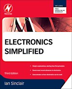
To see just how much of a problem the conversion of sound waves is, imagine a system that used only the numbers −2 to +2, on a signal of 4
V total peak-to-peak amplitude. If this were used to code a waveform (shown as a triangular wave for simplicity) as in Figure 9.1 (a) then since no half-digits can exist, any level between −0.5
V and +0.5
V would be coded as 0, any signal between +0.5
V and +1.5
V as 1 and so on, using ordinary denary numbers rather than binary numbers here to make the principle clearer. In other words, each part of the wave is represented by an integer (whole) number between −2 and +2, and if we plotted these numbers on the same graph scale then the result would look as in Figure 9.1 (b). This is a ‘block’ shape of wave, but recognizably a wave which if heavily smoothed would be something like the original one.
 |
| Figure 9.1 Quantizing a waveform. Each new level of voltage is represented by the number for that level, so that the waveform is coded as a stream of numbers. Reversing the process produces a shape that when smoothed (averaged) provides a recognizable copy of the input even for this very crude five-level system |
We could say that this is a five-level quantization of the wave, meaning that the infinite number of voltage levels of the original wave has been reduced to just five separate levels. This is a very crude quantization, and the shape of a wave that has been quantized to a larger number of levels is a much better approximation to the original. The larger the number of levels, the closer the wave comes to its original pattern, though we are cheating in a sense by using a sinewave as an illustration, since this is the simplest type of wave to convert in each direction; we need know only one number, the peak amplitude, to specify a sinewave. Nevertheless, it is clear that the greater the number of levels that can be expressed as different numbers then the better is the fidelity of the sample.
Definition
Definition
Quantization means the sampling of a waveform so that the amplitude of each sample can be represented by a number. It is the essential first step in converting from analog form to digital form.
In case you feel that all this is a gross distortion of a wave, consider what happens when an audio wave of 10
kHz is transmitted by medium-wave radio, using a carrier wave of 500
kHz. One audio wave will occupy the time of 50 radio waves, which means in effect that the shape of the audio wave is represented by the amplitudes of the peaks of 50 radio waves, a 50-level quantization. You might also like to consider what sort of quantization is involved when an analog tape system uses a bias frequency of only 110
kHz, as many do. Compare this with the 65,536 levels used for a CD.
The idea of carrying an audio wave by making use of samples is not in any way new, and is inherent in amplitude modulation (AM) radio systems which were considered reasonably good for many years. It is equally inherent in frequency modulation (FM), and it is only the use of a fairly large amount of frequency change (the peak deviation) that avoids this type of quantization becoming too crude. Of all the quantized ways of carrying an audio signal, in fact, FM is probably the most satisfactory, and FM methods are often adopted for digital recording, using one frequency to represent a 0 and another to represent a 1. Another option that we shall look at later is changing the phase and amplitude of a wave, with each different phase and amplitude representing a different set of digital bits.
Summary
Summary
The conversion of a waveform into a set of digital signals starts with quantization of the wave to produce a set of numbers. The greater the number of quantization levels, the more precise the digital representation, but excessive quantization is wasteful in terms of the time required.
This brings us to the second problem, however. Because the conversion of an audio wave into a set of digits involves sampling the voltage of the wave at a large number of intervals, the digital signal consists of a large set of numbers. Suppose that the highest frequency of audio signal is sampled four times per cycle. This would mean that the highest audio frequency of 20
kHz would require a sampling rate of 80
kHz. This is not exactly an easy frequency to record even if it were in the form of a sinewave, and the whole point of digital waveforms is that they are not sinewaves but steep-sided pulses which are considerably more difficult to record. From this alone, it is not difficult to see that digital recording of sound must involve rather more than analog recording.
The next point is the form of the numbers. We have seen already that numbers are used in binary form in order to allow for the use of only the two values of 0 and 1. The binary code that has been illustrated in this chapter is called 8-4-2-1 binary, because the position of a digit represents the powers of two that follow this type of sequence. There are, however, other ways of representing numbers in terms of 0 and 1, and the main advantage of the 8-4-2-1 system is that both coding and decoding are relatively simple. Whatever method is used, however, we cannot get away from the size that the binary number must have. It is generally agreed that modern digital audio for music should use a 16-bit number to represent each wave amplitude, so that the wave amplitude can be any of up to 65,536 values. For each sample that we take of a wave, then, we have to record 16 digital signals, each 0 or 1, and all 16
bits will be needed in order to reconstitute the original wave. We refer to this as a
bit-depth of 16. Bit-depths higher than this are used for professional equipment; a bit-depth of 24 is typical.
Definition
Definition
A bit is short for a binary digit, a 0 or 1 signal. By convention, bits are usually gathered into a set of eight, called a
byte. A pair of bytes, 16 bits, is called a
word. Unfortunately, the same term is also used for higher number groupings such as 32, 64, 128, etc.
Digital Coding
The number of digital signals per sample is the point on which so many attempts to achieve digital coding of audio have foundered in the past. As so often happens, the problems could be more easily solved using tape methods, because it would be quite feasible to make a 16-track tape recorder using wide tape and to use each channel for one particular bit in a number. This is, in fact, the method that can be used for digital mastering where tape size is not a problem, but the disadvantage here is that for original recordings some 16–32 separate music tracks will be needed. If each of these were to consist of 16 digital tracks the recorder would, to put it mildly, be rather overloaded. Since there is no possibility of creating or using a 16-track disc, the attractively simple idea of using one track per digital bit has to be put aside. The alternative is
serial transmission and recording.
Definition
Definition
Serial means one after another. For 16 bits of a binary number, serial transmission means that the bits are transmitted in a stream of 16 separate signals of 0 or 1, rather in the form of separate signals on 16 channels at once. The rate of transmission of a digital serial signal is stated in kb/s (kilobits per second) or Mb/s (megabits per second).
Now if the signals are samples that have been taken at the rate of 40
kHz, and each signal requires 16 bits to be sent out, then the rate of sending digital signals is 16
×
40 kb/s, which if we coded it as one wave per bit would be equivalent to a frequency of 640
kHz, well beyond the rates for which ordinary tape or disc systems can cope. As it happens, we can get away with much more efficient coding and with slower sampling rates, as we shall see, but this does not offer much relief because there are further problems.
Note
Note
A well-known rule (Shannon’s law, which was worked out long before digital recording was established) states that the sampling rate must be at least twice the highest component of the analog signal, so that a 40
kHz sampling rate is adequate for a signal whose highest frequency is 20
kHz. Remember that the components of an audio signal that are at this highest frequency will be present only in very small amplitudes.
When a parallel system is used, with one channel for each bit, there is no problem of identifying a number, because the bits are present at the same time on the 16 different channels, with each bit in its place; the most significant bit will be on the MSB line, the least significant on the LSB line, and so on. When bits are sent one at a time, though, how do you know which bits belong to which number? Can you be sure that a bit is the last bit of one number or is it the first bit of the next number? The point is very important because when the 8-4-2-1 system is used, a 1 as the most important bit means a value of 32,768, but a 1 as the least important bit means just 1. The difference in terms of signal amplitudes is enormous, which is why binary codes other than the 8-4-2-1 type are used industrially. The 8-4-2-1 code is used mainly in computing because of the ease with which arithmetical operations can be carried out on numbers that use this code.
Even if we assume that the groups of 16 bits can be counted out perfectly, what happens if one bit is missed or mistaken? At a frequency of 1
MHz or more it would be hopelessly optimistic to assume that a bit might not be lost or changed. There are tape dropouts and dropins to consider, and discs cannot have perfect surfaces. At such a density of data, faults are inevitable, and some methods must be used to ensure that the groups of 16 bits (
words) remain correctly gathered together. Whatever method is used must not compromise the rate at which the numbers are transmitted, however, because this is the sampling rate and it must remain fixed. Fortunately, the problems are not new nor unique to audio; they have existed for a long time and been tackled by the designers of computer systems. A look at how these problems are tackled in simple computer systems gives a few clues as to how the designers of audio digital systems went about their task.
Summary
Summary
The problem of conversion from analog to digital signals for sound waves is the rate of conversion that is needed. The accepted number of digits per sample is 16, and Shannon’s law states that the sampling rate must be at least twice the highest component of the analog signal. For a maximum of 20
kHz, this means a sampling rate of 40
kHz, and for 16-bit signals, this requires a rate of 16
×
20 thousand bits per second, which is 320,000 bits per second. These bit signals have to be recorded and transmitted in serial form, meaning one after another.
Analog to Digital
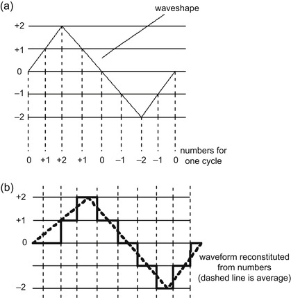
Converting from an analog into a digital signal involves the quantization steps that have been explained above, but the mechanism needs some explanation in the form of block diagrams. All analog to digital (A/D) conversions start with a sample and hold circuit, illustrated in block form in Figure 9.2.
 |
| Figure 9.2 An elementary sample and hold circuit, using a switch to represent the switching actions that would be carried out using metal-oxide-semiconductor field-effect transistors (MOSFETs). When the switch opens, the voltage on the capacitor is a sampled waveform voltage for that instant, and the conversion to digital form of this voltage at the output of the sample and hold circuit must take place before the next sample is taken |
The input to this circuit is the waveform that is to be converted to digital form, and this is taken through a buffer stage to a switch and a capacitor. While the switch is closed, the voltage across the capacitor will be the waveform voltage; the buffer ensures that the capacitor can be charged and discharged without taking power from the signal source. At the instant when the switch opens, the voltage across the capacitor is the sampled waveform voltage, and this will remain stored until the capacitor discharges. Since the next stage is another buffer, it is easy to ensure that the amount of discharge is negligible. While the switch is open and the voltage is stored, the conversion of this voltage into digital form (quantization) can take place, and this action must be completed before the switch closes again at the end of the sampling period.
In this diagram, a simple mechanical switch has been indicated but in practice this switch action would be carried out using MOSFETs which are part of the conversion IC. To put some figures on the process, at the sampling rate of 44.1
kHz that is used for CDs, the hold period cannot be longer than 22
ms, which looks long enough for conversion – but read on!
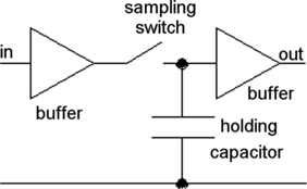
The conversion can use a circuit such as is outlined in Figure 9.3 and which very closely resembles the diagram of a digital voltmeter illustrated in Chapter 11. The clock pulses are at a frequency that is much higher than the sampling pulses, and while a voltage is being held at the input, the clock pulses pass through the gate and are counted. The clock pulses are also the input to the integrator, whose output is a rising voltage. When the output voltage from the integrator reaches the same level (or slightly above the level) as the input voltage, the gate shuts off, and the counted number at this point is used as the digital signal. The reset pulse (from the sample and hold switch circuit) then resets the counter and the integrator so that a new count can start for the next sampled voltage.
 |
| Figure 9.3 A typical analog to digital (A/D) converter. The gate passes clock pulses that are integrated until the output of the integrator equals the comparator input voltage. The pulse count is the output of the counter, the digital signal. The circuit then resets for the next count |
The clock pulse must be at a rate that will permit a full set of pulses to be counted in a sampling interval. For example, if the counter uses 8-bit output, corresponding to a count of 65,538 (which is 2
8), and the sampling time is 20
ms, then it must be possible to count 65,536 clock pulses in 20
ms, giving a clock rate of 3.27
GHz. This is not a rate that would be easy to supply or to work with (though rates of this magnitude are now commonplace in computers), so that the conversion process is not quite as simple as has been suggested here. For CD recording, more advanced A/D conversion methods are used, such as the successive approximation method (in which the input voltage is first compared to the voltage corresponding to the most significant digit, then successively to all the others, so that only eight comparisons are needed for an 8-bit output rather than 65,536). If you are curious about these methods, see the book
Introducing Digital Audio from PC Publishing.
Note
Note
The sampling rate for many analog signals can be much lower than the 44.1
kHz that is used for CD recording, and most industrial processes can use much lower rates. ICs for these A/D conversions are therefore mostly of the simpler type, taking a few milliseconds for each conversion. Very high-speed (
flash) converters are also obtainable that can work at sampling rates of many megahertz.
Digital to Analog
Converting digital to analog is easy enough if a small number of bits are being used and if the rate of conversion is low. Figure 9.4 shows a simple method that uses an operational amplifier for a 4-bit digital signal. If we imagine that the switches represent a set of digital inputs (closed
=
1, open
=
0) then the digital signals will close or open feedback paths for the operational amplifier, so that the output voltage will be some multiple of the input (reference) voltage) that is set by the total resistance in the feedback path. In practice, of course, the switches are MOSFETs which are switched on or off by the digital inputs on four lines in this example.
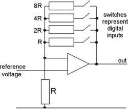 |
| Figure 9.4 A simple voltage-adding digital to analog (D/A) converter |
Though this system is adequate for 4-bit conversions, it presents impossible problems when you try to use it for 8 or more bits. The snag is that the resistor values become difficult to achieve, and the tolerance of resistance is so tight that manufacturing is expensive. Other methods have therefore been devised, such as current addition and bitstream converters, both beyond the scope of this book. Converters for 16 bits are now readily available at reasonable prices. Flash conversion is dealt with in Chapter 12.
Summary
Summary
Conversion between analog and digital signals is straightforward if sampling rates are low and the number of bits is small. More elaborate methods are needed for fast conversion and for 16-bit operation, but the problems have been solved by the IC manufacturers and a large range of conversion ICs can be bought off the shelf.
Serial Transmission
To start with, when computers transmit data serially, the word that is transmitted is not just the group of digits that is used for coding a number. For historic reasons, computers transmit in units of 8-bit bytes, rather than in 16-bit words, but the principles are equally valid. When a byte is transmitted over a serial link, using what is called
asynchronous methods, it is preceded by one
start bit and followed by one or two (according to the system that is used)
stop bits.
Since the use of two stop bits is very common, we will stick to the example of one start bit, eight number bits and two stop bits. The start bit is a 0 and the stop bits are 1s, so that each group of 11 bits that are sent will start with a 0 and end with two 1s. The receiving circuits will place each group of 11 bits into a temporary store and check for these start and stop bits being correct. If they are not, then the digits as they come in are shifted along until the pattern becomes correct. This means that an incorrect bit will cause loss of data, because it may need several attempts to find that the pattern fits again, but it will not result in every byte that follows being incorrect, as would happen if the start and stop bits were not used.
The use of start and stop bits is one very simple method of checking the accuracy of digital transmissions, and it is remarkably successful, but it is just one of a number of methods. In conjunction with the use of start and stop bits, many computer systems also use what is known as
parity, an old-established method of detecting one-bit errors in text data. In a group of eight bits, only seven are normally used to carry text data (in ASCII code) and the eighth is spare. This redundant bit is made to carry a checking signal, which is of a very simple type.
We can illustrate how it works with an example of what is termed
even parity. Even parity means that the number of 1s in a group of eight shall always be even. If the number is odd, then there has been an error in transmission and a computer system may be able to make the transmitting equipment try again. When each byte is sent the number of 1s is counted. If this number is even, then the redundant bit is left as a 0, but if the number is odd, then the redundant bit is made a 1, so that the group of eight now contains an even number of 1s. At the receiver, all that is normally done is to check for the number of 1s being even, and no attempt is made to find which bit is at fault if an error is detected. The redundant bit is not used for any purpose other than making the total number even. The process is illustrated in Table 9.2.
Parity, used in this way, is a very simple system indeed, and if two bits in a byte are in error it is possible that the parity could be correct though the transmitted data was not. In addition, the parity bit itself might be the one that was affected by the error so that the data is signaled as being faulty even though it is perfect. Nevertheless, parity, like the use of start bits and stop bits, works remarkably well and allows large masses of computer text data to be transmitted over serial lines at reasonably fast rates. What is a reasonably fast rate for a computer is not, however, very brilliant for audio, and even for the less demanding types of computing purposes the use of parity is not really good enough and much better methods have been devised. Parity has now almost vanished as a main checking method because it is now unusual to send plain (7-bit) text; we use formatted text using all 8 bits in each byte, and we also send coded pictures and sound using all 8 bits of each byte, so that an added parity bit would make a 9-bit unit (not impossible but awkward, and better methods are available).
The rates of sending bits serially over telephone lines in the pre-broadband days ranged from the painfully slow 110 bits per second (used at one time for teleprinters) to the more tolerable 56,000 bits per second. Even this fast rate is very slow by the standards that we have been talking about, so it is obvious that something rather better is needed for audio information. Using direct cable connections, rates of several million bits per second can be achieved, and these rates are used for the universal serial bus (USB) system that is featured in modern computers. We will look at broadband methods later.
As a further complication, recording methods do not cope well with signals that are composed of long strings of 1s or 0s; this is equivalent to trying to record square waves in an analog system. The way round this is to use a signal of more than 8 bits for a byte, and using a form of conversion table for bytes that contain long sequences of 1s or 0s. A very popular format that can be used is called eleven-to-fourteen (ETF), and as the name suggests, this converts each 11-bit piece of code (8 bits of data plus 3 bits used for error checking) into 14-bit pieces which will not contain any long runs of 1s or 0s and which are also free of sequences that alternate too quickly, such as 01010101010101.
All in all, then, the advantages that digital coding of audio signals can deliver are not obtained easily, whether we work with tape or with disc. The rate of transmission of data is enormous, as is the bandwidth required, and the error-detecting methods must be very much better and work very much more quickly than is needed for the familiar personal computers that are used to such a large extent today. That the whole business should have been solved so satisfactorily as to permit mass production is very satisfying, and even more satisfying is the point that there is just one worldwide CD standard, not the furiously competing systems that made video recording such a problem for the consumer in the early days.
For coding television signals, the same principles apply, but we do not attempt to convert the analog television signal into digital because we need only the video portion, not the synchronization pulses. Each position on the screen is represented by a binary number which carries the information on brightness and color. Pictures of the quality we are used to can be obtained using only 8 bits. Once again, the problems relate to the speed at which the information is sampled, and the methods used for digital television video signals are quite unlike those used for the older system, though the signals have to be converted to analog form before they are applied to the guns of a cathode-ray tube (CRT). Even this conversion becomes unnecessary when CRTs are replaced by color liquid crystal display (LCD) screens, because the IC that deals with television processing feeds to a digital processor that drives the LCD dots.
A more detailed description and block diagram of CD replay systems is contained in Chapter 12.
Summary
Summary
Digital coding has the enormous advantage that various methods can be used to check that a signal has not been changed during storage or transmission. The simplest system uses parity, adding one extra bit to check that number of 1s in a byte. More elaborate systems can allow each bit to be checked, so that circuits at the far end can correct errors. In addition, using coding systems such as ETF can avoid sequences of bits that are difficult to transmit or record with perfect precision.
..................Content has been hidden....................
You can't read the all page of ebook, please click here login for view all page.