Chapter 4. Linear Circuits
Linear circuits and amplification. Gain and its measurement. Linearity and forms of non-linearity. Distortion and causes of distortion. Attenuation of signal. Transistor (BJT or MOSFET) as a linear amplifier. Buffer (zero-gain) circuits. Decibel scale and its use. Misuse of decibel quantities. Frequency response of a linear amplifier. Bandwidth and its measurement. Audio bandwidth range. Broadband amplifiers. Tuned amplifiers. Radio carrier and amplitude modulation (AM). Frequency modulation (FM). Broadening bandwidth of tuned amplifiers by damping or stagger tuning. Power and RMS values for AC and signals. Calculation of power for sinewave. Form factor for non-sine waves. Peak and RMS values. Feedback of signal in an amplifier. Oscillation caused by positive feedback. Negative feedback. Oscillators and multipliers. Untuned oscillators. Frequency multipliers.
Linearity
We have seen that there are two main types of electronic circuits, and we label them as
analog or as
digital circuits. Though we can design and construct both types of circuits using the same set of active and passive components, the active components are used in very different ways and the waveforms that are processed are very different.
Note
Note
Analog circuits are not necessarily linear – a rectifier circuit is just one example – and such non-linear circuits are not digital. We class these circuits as
non-linear analog circuits. In short, all linear circuits are analog, but not all analog circuits are linear.
A linear circuit is a type of analog circuit that is designed to make a
scaled copy of a waveform, and by scaled we mean that the amplitude of the output of the linear circuit is a fraction or a multiple of the amplitude of the input waveform. The output amplitude might be smaller, in which case we often call the circuit an
attenuator. The output amplitude might be equal, in which case we usually call the circuit a
buffer. Quite commonly the output amplitude is greater than the input amplitude, and the circuit is an
amplifier. If the circuit is truly linear, the output waveform has the same frequency and the same
waveshape as the input waveform – it is a true copy at a different amplitude scale (Figure 4.1), and the ratio of the output amplitude to the input amplitude is called the
gain.
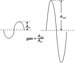 |
| Figure 4.1 Amplitude and gain. The amplitudes must be measured in the same way, and peak amplitude measurements are illustrated here |
The name of
linear circuit arises from the shape of graphs of output amplitude plotted against input amplitude. For a perfectly linear amplifier, this graph should be a straight line, hence the name
linear. As it is, because of the imperfections of active components, amplifiers are never perfectly linear, though we can obtain very good linearity in a buffer circuit, and perfect linearity in an attenuator which uses only passive components. Figure 4.2 shows perfect linearity and some common varieties of imperfections in graphs for amplifiers.
Note
Definition
Note
A graph cannot show small amounts of non-linearity, and we have to use instruments to detect traces of non-linearity by other methods. One such method is to use a perfect sinewave as an input; any non-linearity will cause the output to contain harmonics, waves at higher frequencies, and these can be detected by sensitive instruments.
Definition
A linear circuit is one for which a graph of output plotted against input is a straight line. Linear circuits are used in analog designs, though not all analog circuits need be perfectly linear.
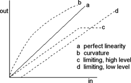 |
| Figure 4.2 Linear and non-linear behavior of amplifiers |
The most common imperfection is curvature: the graph line is curved rather than straight. This means that the amount of gain, the scaling, alters as the input amplitude alters. For example, large-amplitude signals may be amplified less than small-amplitude signals. This type of non-linearity is sometimes required, and the human ear itself is non-linear, a way of protecting us from the worst effects of the noise of explosions, aircraft noise, and discos.
In general, though, for purposes such as sound reproduction, we need amplifiers that are as linear as we can get them, and a target of 0.1% deviation from a straight-line graph is taken as a reasonable target for a hi-fi amplifier. This deviation from linearity is often called the
distortion figure, and quite high distortion figures (of 10% or more) are common for radios, compact disc (CD) players, guitar amplifiers, disco amplifiers, and other equipment for which high-quality reproduction is not an important factor.
Another imperfection that is illustrated in the drawing is
limiting. When an amplifier limits, the output amplitude stays constant even though the input amplitude is changing. This causes the shape of the waveform at the output to be severely distorted, flattening at the tops as in Figure 4.3. All amplifiers will limit if the input amplitude is too large, so that a complete amplifier system has to be designed so that limiting cannot occur even if the volume control is turned full up. If an amplifier is designed to have different input amplitudes, as it must if it is supplied from different sources such as tape-heads, pickups, radio circuits, CD players, etc., then there should be adjustments provided so that the manufacturer or user can set each input to the same level so that the master volume control does not need to be adjusted when you switch from one source to another. It is unusual to find these adjustments provided except on expensive sound equipment.
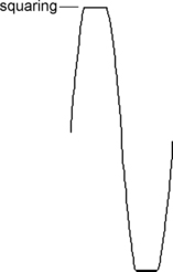 |
| Figure 4.3 Squaring is the effect on the waveform of some type of limiting action in an amplifier |
The third type of non-linear behavior illustrated is another form of limiting. The amplifier simply does not amplify signals that are at a very low-amplitude level. This type of non-linearity has in the past been used deliberately to reduce the noise signals from cassette tapes but, like the other types, it is undesirable in normal use. When transistor amplifiers first appeared, a form of this type of distortion, called
cross-over distortion, was a common fault which delayed the acceptance of transistors for high-quality linear amplifiers until solutions were found.
Summary
Note
Summary
Non-linear behavior includes curvature and limiting. Though these effects are sometimes deliberately used, high-quality amplifier designers aim to reduce non-linearity to as low as can economically be attained. The amount of non-linearity is often expressed as the percentage by which the graph line deviates from a straight line, and a usual target for high-quality amplifiers is 0.1%, one part in 1000 (though this figure cannot be obtained from a graph).
Note
Some devotees of hi-fi are not necessarily logical in their choice, and some prefer to hear the type of distortion (often large) that is caused when the old-fashioned vacuum tube amplifiers are used. Others are prepared to believe that they can hear differences caused by the type of wire used for connecting cables. One more skeptical authority has commented that the only significant difference cables can make to loudspeaker performance is if they are too short to reach the loudspeakers. The most sensible advice is to avoid the type of magazines that use the sort of fancy descriptions that are employed by wine tasters or art reviewers.
An attenuator that is constructed entirely from passive components, such as the type shown in Figure 4.4, is perfectly linear for the normal signals that we are concerned with. This is because non-linearity is caused almost exclusively by active components. Passive components contribute to non-linearity only if they are overloaded, and that is reasonably easy to avoid.
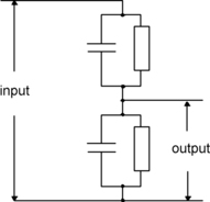 |
| Figure 4.4 An attenuator formed from passive components does not cause any non-linear distortions. The type illustrated here is a compensated attenuator which will work over a very wide range of frequencies |
The root causes of non-linearity in bipolar transistor circuits are:
• A simple plot of collector wave voltage against base wave voltage for a transistor in a simple amplifier circuit (Figure 4.5) is curved.
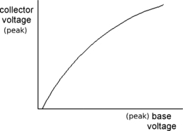 |
| Figure 4.5 The non-linear behavior of a transistor at its worst. Correct bias and choice of transistor type can help, but the graph shape is always a curve. Note that what is being plotted is the peak amplitude of the waves at input and output |
• There is no collector output for small base waveforms.
The same considerations apply to metal-oxide-semiconductor field-effect transistor (MOSFET) circuits, though MOSFETs can be manufactured so that they have more linear input/output graphs. Careful attention to transistor biasing and circuit design can result in a graph shape that is closer to a straight line, eliminating the region where there is no collector or drain output, but there is always some curvature. The problem is tackled by cunning circuit design that applies corrections to the output wave (a system called
negative feedback), but this is not in itself a way of making a poorly designed amplifier perfect; though it can make a good design work better.
Note
Note
Good design of operational amplifiers can also reduce distortion to a very low figure provided that there is no overloading in any part of the amplifier.
Yet another type of distortion is called
slew-rate limiting, and it is quite different from the others. Slew-rate limiting occurs in a transistor, whether it is a separate transistor or part of an integrated circuit (IC), and it cannot be eliminated by circuit design, only by using transistors that have better design characteristics. Imagine a simple single-transistor amplifier. For a small input this may be able to cope with a waveform that has a sudden change in voltage, but if the change in voltage at the input is large the transistor simply cannot pass enough current at the output to charge or discharge stray capacitance. The effect is that the change in voltage at the output takes longer or is limited. This effect is most likely to be a problem for power amplifiers, and the solution is either to filter out any inputs that have large sudden voltage changes, or to use different types of semiconductors in the active part of the circuit.
Summary
Summary
Slew-rate limiting affects amplifiers that handle inputs with sudden voltage changes where the change of voltage can be large. The effect causes a form of distortion (because the waveshape is changed) that can be eliminated only by using better semiconductor types.
A
buffer circuit makes use of an active component circuit controlled by passive components, but with the output amplitude the same as (or slightly less than) the input amplifier. For this type of action, it is possible to make transistors work in a fairly linear way so that distortion can be very small, though never zero. The purpose of a buffer is to prevent
loading of a signal. For example, suppose that the input to an amplifier is a signal of 1
mV which can supply only 1
μA of signal current. Now if we connect this to an amplifier which needs to pass 10
μA at its input, we are asking too much of the signal source, loading it, and this is certain to cause non-linear behavior.
If we place a buffer stage between the amplifier and the source, using a buffer which takes a current much less than 1
μA of current but can provide more than 10
μA at its output, then we avoid the loading effect and improve the performance of the whole amplifier. Buffers are used in all types of circuits, linear and digital, for this same purpose, to avoid taking more current from a signal source than it can comfortably supply. Another function of a buffer is to isolate two stages so that the signals in the second stage cannot affect the first stage.
The simplest type of transistor buffer circuit is illustrated in Figure 4.6, using a bipolar transistor. This is called an
emitter-follower, and the output signal voltage is in phase with the input. The amplitude of the output is slightly less than the amplitude of the input, but the power output is more because the emitter current of the transistor can be much greater than the base current. This is an example of 100% negative feedback (see later in this chapter), because the input to the transistor is the voltage between base and emitter, but this is equal to the input signal (between base and earth) minus the output signal between emitter and earth. The MOSFET equivalent is the
source-follower.
Summary
Summary
Buffers are linear circuits with zero gain, and it is fairly easy to ensure that they are almost perfectly linear. Buffers prevent too much current being taken from the source of a signal, and are used to isolate one section of a circuit from the next. The emitter-follower type of circuit is a simple type of buffer, and an opamp equivalent, the voltage-follower, is widely used.
 |
| Figure 4.6 An emitter-follower circuit, a simple example of a buffer that provides power gain without voltage gain |
Gain
An amplifier carries out the action of making an enlarged copy of the waveform that is used as its input signal, and the ratio of the output signal to the input signal is called the
gain of the amplifier. This figure of gain could be written, for example, as ×10, ×100, or even ×1000, but we seldom use this way of expressing gain.
Definition
Definition
Voltage gain is defined as (output signal voltage)/(input signal voltage). We can also define
power gain as (output power)/(input power), or
current gain as (output current)/(input current).
Expressing gain as a simple ratio of voltages is often useful, particularly if we are aiming for some definite signal output level such as 0.5
V RMS (root mean square; see later), but for amplifiers that deal with signals in sound or vision systems, the
decibel scale is more useful. There is nothing mysterious about it, except that it is often misused. We have known for more than a century that human ears and eyes do not have a linear response. For example, when the amplitude of two sound waves is compared, one with twice the amplitude of the other, your ears do not hear one sound as twice as loudly as the other. Similarly, two lights, one with twice the amplitude of the other, do not appear to your eyes so that one looks twice as bright as the other.
The type of scale that your senses use is
logarithmic, meaning that the quantity we perceive is related to the logarithm of the wave amplitude. These logarithm units of comparison are called
decibels, named after Alexander Graham Bell, who we remember for the invention of the telephone, but whose main interest in life was the problem of deafness; in fact, the first telephone was invented as an aid for the deaf.
Definition
Definition
If one voltage amplitude is 100 times the size of another, our senses tell us that when signal amplitude is converted into sound or light the ratio is something more like 40 times, which is 20 times the logarithm of 100. As a formula this is 20 log (
GV), where G
V is the simple voltage gain. If this is applied to power gains, it becomes 10 log (
GP), where G
P is the simple power gain.
A voltage amplifier is very likely to be specified with its figure of gain expressed in decibels, abbreviation dB. A decibel gain of 40
dB corresponds to a voltage gain of 100 (and a power gain of 10,000). Table 4.1 shows some values of voltage gain ratios and decibel amounts.
Note
Note
Strictly speaking, decibels should be used only for comparing power levels, using the 10 log (
GP) formula. The use of decibels for comparing voltages, however, is so common that it cannot be ignored, though it is really valid only when the voltages are measured across the same value of resistance (which implies that the current has been amplified as much as the voltage).
The trap to watch for is that a decibel value always refers to a
ratio. You cannot, for example, say that a noise is at 100
dB unless you specify what your comparison is. A figure of 100
dB means that the noise is that much louder than something else, but you have to specify what that something else is. There are agreed comparisons for sound, but they are based on measured power rather than something subjective like a demented fly at 20 feet.
The gain of an amplifier is a ratio and is therefore always specified in decibels, and this form is also used for attenuators. For example, you might specify a −10
dB attenuation, meaning that the output voltage is only about 0.3 times the input voltage. The minus sign indicates that this is a ratio of input to output, not output to input, with the output amplitude less than the input amplitude.
Summary
Summary
Because our senses work on a logarithmic scale, it is often more convenient to express gain in this way, and this is the purpose of the decibel scale. For power gain, the number of decibels is equal to 10 log (
GP), where
GP is the power gain, and this is the true definition of the number of decibels. For many purposes, however, it is convenient to work in voltage terms, and the number of decibels corresponding to a voltage gain is 20 log (
GV), where
GV is the voltage gain.
Frequency Response
The graph of output amplitude plotted against input amplitude shows up gross non-linear behavior, but there is another form of distortion that can affect any linear amplifier, and even passive devices such as attenuators. This is
frequency distortion. Some amplifiers are intended to work with a single frequency or a narrow band of frequencies. These are tuned amplifiers and we shall look at them later in this chapter. More usually, an amplifier has to work for a range of frequencies, and it must have the same amount of gain for all the frequencies in that range, which is its
bandwidth.
For example, an amplifier that is used along with a CD player should be able to deal with the frequency range of about 30
Hz to 20
kHz, the
audio range. These frequencies represent the limits of a (young) human ear, and as we get older our ability to hear the higher frequencies is steadily reduced; one estimate is that the rate is 1
Hz less each day, so that the upper limit can eventually be as low as 10
kHz or less. The human ear is at its most sensitive at a frequency of around 330
Hz (the average frequency of the female voice), and sensitivity is reduced at the very low as well as the very high ends of the frequency range. An amplifier designed to deal with the normal audio frequency range is an
audio amplifier. This is the most common form of amplifier because every radio, mobile phone, cassette, MP3 or CD player, and television receiver, includes an audio amplifier stage.
A typical graph of gain plotted against frequency for an audio amplifier is illustrated in Figure 4.7. The gain is displayed in dB units, and the frequency is shown on a logarithmic scale, so that the markings are 1, 10, 100, 1000, and so on, at equal intervals. This type of graph is called a
frequency response graph.
Definition
Note
Definition
A logarithmic scale is one that uses a fixed
distance to represent a fixed
multiple. For example, you might use 1
cm on the graph to represent each ten-fold change in a quantity leading to a 1, 10, 100, 1000 scale, with these numbers at equal intervals. On such a scale, the mark midway between 10 and 100 does
not represent 50 (it is closer to 31).
Note
If we used a linear scale, with the distance proportional to the frequency, the length of the frequency scale would be ridiculous. For example, if we allowed 1
cm for 10
Hz, the length of the scale in this example would be about 2000
cm. In addition, because the decibel scale is logarithmic, it makes sense to use this type of scale also for frequency.
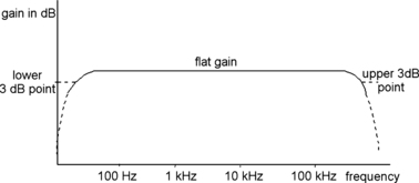 |
| Figure 4.7 A frequency response graph, showing the 3
dB points, between which the bandwidth is measured |
In the example, the frequency response is level for most of the range, with a downturn at each end. The convention is to take the frequency response as extending between the points where the level is 3
dB below the flat (maximum) portion. The basis of this is that 3
dB is an amount of change that in terms of sound or light is only just significant and noticeable to ears or eyes, so we can ignore variations of less than this amount. Even if the frequency response graph has no flat portion, we can ignore variations that are less than 3
dB. One of the advantages of using the decibel scale is that this amount of variation looks small on the graph: a 3
dB variation in terms of gain means a two-fold change (twice or half), which would look very large on a linear graph, but does not have so much of an impact on ear or eye.
Definition
Definition
The bandwidth of an amplifier is defined as the range of frequencies between which the change in gain is 3
dB. For audio amplifiers, this is usually quoted in terms of a range of frequencies, such as 20
Hz to 20
kHz. For radio frequency amplifiers (see later) this will be expressed as the
difference between the frequencies, such as 5
kHz, 100
kHz, 5.5
MHz, and so on.
No amplifier can have a perfectly flat frequency response over a really large range of frequencies. The use of capacitors to carry signals between sections of a circuit limits the gain figure for the low frequencies, because the reactance of a capacitor is high for a signal at a low frequency. There are also limits on the gain that can be achieved at high frequencies, caused by transistors themselves and by stray capacitance. Stray capacitance is unplanned capacitance between different parts of the circuit, and this arises because a capacitor is an insulator sandwiched between conductors, so that any two pieces of metal separated by air must have some capacitance. These strays filter off the highest frequencies because even a small value of capacitance will have a low reactance for signals at high frequencies. In some circuits the design of the circuit is able to compensate for such losses. In other circuits there may be hills and dales on the frequency response graph because of
resonance effects caused by stray capacitances and stray inductances.
Broadband Amplifiers
There is a special class of linear amplifiers called
broadband amplifiers. This name is reserved for amplifiers that have a much wider frequency response than the ordinary audio amplifier. For example, the waveform that carries the picture information (for an analog television receiver, for example) is called the
video signal. Ideally, an amplifier for this signal should have a bandwidth of zero to around 5.5
MHz (
zero means that changes in the steady voltage level are also amplified). In such a signal, there is a DC portion which carries the information on the overall brightness of the screen, while the highest frequencies carry the information on the finest detail.
This bandwidth is much greater than is used for audio signals, and to put it in perspective, it is more than five times as much as the whole of the medium-wave band on a radio. Even this, however, is small compared with some other bandwidths. A good computer monitor, for example, will use an 80
MHz bandwidth, which is why we once used (costly) cathode-ray tube (CRT) monitors for computers rather than (cheap) CRT television receivers, and why computer images that look so clear on a good monitor look so fuzzy on a television screen. Now that both monitors and television screens use flat-screen digital display methods the differences are much less. Some measuring instruments that are used to find the amplitude and frequency of waveforms need amplifiers with a bandwidth of 100
MHz or more.
These broadband amplifiers need to be designed with great care, and the physical arrangement (
layout) of the components is just as important as the theoretical design of the circuit. Very large bandwidths are also used in connection with the amplifiers that are used for receiving radio signals, particularly the low-noise box (
LNB) amplifiers that are contained in satellite receiving dishes.
Tuned Amplifiers
The broadband amplifiers that are used, for example, in a computer monitor or an oscilloscope are classed as
untuned (or
aperiodic) amplifiers, but we also make considerable use of
tuned amplifiers. Recalling Chapter 2, a combination of an inductor and a capacitor is a tuned circuit that has a peak response at some frequency. This value of frequency, the tuned frequency, can be calculated from the amounts of inductance and capacitance, but the response of the circuit shows some gain for a range of frequencies around the tuned frequency. As usual, the bandwidth is calculated as the frequency range between the points where the response is 3
dB down (the −3
dB points) (Figure 4.8).
Definition
Definition
A tuned amplifier is one whose bandwidth is centered around a single frequency (or center
frequency) at which the response is maximum. This is usually achieved using resonant circuits in conjunction with active components.
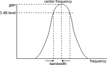 |
| Figure 4.8 The bandwidth for a tuned circuit is measured to one of the 3
dB points on either side of the tuned (center) frequency |
Bandwidth is important, because it affects the use that we can make of radio waves. As we will see in Chapter 6, a radio transmission makes use of a small band of frequencies that lie around a central maximum which is the frequency set at the transmitter (the
carrier frequency). This bandwidth for medium-wave broadcasts is only about 5
kHz on each side of the tuned frequency. This, in turn, means that the frequency range for sound on medium-wave radio is only about 5
kHz. This situation has arisen because too many transmitters use the medium waves. As far as speech is concerned, this 5
kHz is adequate, but it is nothing like adequate for the good reproduction of music (or the reproduction of good music). In addition, the older methods of using a radio wave to carry sound signals (modulation methods) are very susceptible to interference both from natural (e.g. lightning) and artificial (e.g. car ignition systems) causes.
This problem has been around for a long time, and it was first solved by an amazing US genius called Armstrong (whose other inventions have also been landmarks in radio). In the 1930s, Armstrong developed a method, called
frequency modulation (FM), for carrying high-quality sound on radio waves. This, however, requires a bandwidth of about 100
kHz, so that we need to be able to construct tuned amplifiers with this range of bandwidth for FM radio use. The size of the bandwidth also makes FM unsuitable for medium-wave broadcasts, and carrier frequencies in the 90–110
MHz range have been used.
The most recent solution for high-quality radio broadcasting is
digital radio, and this makes much more efficient use of bandwidth than FM (estimated at about three times more efficient). Digital radio broadcasting allows a bandwidth to carry more than one broadcast so that a set of different channels can be accommodated. Television requires considerably larger bandwidths, and a typical (analog) television broadcast might use a tuned frequency of 800
MHz, using a bandwidth of about 6
MHz. Digital television can, contrary to what you might expect, use smaller bandwidths because of the use of
compression and multiplexing (see Chapter 16).
The simple tuned circuit, as noted in Chapter 2, cannot easily provide such large bandwidths, so various circuit tricks have been used to broaden the bandwidth. All of these methods sacrifice gain so as to obtain more bandwidth, and the simplest is to connect resistors across tuned circuits. These are called
damping resistors, and their action, as illustrated in the graph of Figure 4.9, is to reduce the gain of the tuned circuit but broaden the bandwidth. The reduction in gain can, if necessary, be overcome by increasing the number of tuned amplifying stages.
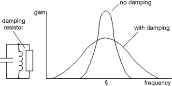 |
| Figure 4.9 The effect of adding a damping resistor to a tuned circuit is to broaden the bandwidth and reduce the gain |
Another method of increasing bandwidth but maintaining gain is to use several tuned stages, but with each tuned to a different frequency around the central frequency. This is called
stagger tuning and, along with damping, it can provide the wide band amplification that is needed for the reception of television signals (the broadband amplifier for video is used at a later stage; see Chapter 8).
One important point about tuned amplifiers is that they need not be particularly linear, though they are classed as linear amplifiers. Any tuned amplifier uses a tuned circuit as a load, and even if the amplifier limits, cutting off part of the wave, the tuned circuit will complete the wave. This is because a tuned circuit acts like a pendulum which, once set into motion, keeps swinging. The tuned circuits are used as loads, and once a transistor has started to pass a wave of current through the tuned circuit, the voltage across the tuned circuit will be a complete wave even if the transistor stops passing current for part of the time.
Summary
Summary
Tuned amplifiers use resonant circuits tuned to a particular frequency, and the circuits can be arranged to give whatever bandwidth is required. Quite simple circuits can provide narrow bandwidths, but for wide bandwidths or several megahertz more elaborate designs are needed.
Power and Root Mean Square Values
Using a linear voltage amplifier on a feeble signal will result in an output that is a signal at a much higher voltage level, but we cannot necessarily use this signal to operate devices such as a loudspeaker or an electric motor. The reason is that these devices need a substantial amount of current passed through them as well as the voltage across their terminals, and a voltage amplifier cannot supply large currents. What we need is a
power amplifier.
For example, a voltage amplifier might provide an output that was a voltage wave of 6
V which could supply no more than 1
mA of current. The power amplifier might provide a wave with a voltage of 6
V and a current of 2
A.
Note
Note
The name of
power amplifier is misleading, because
any amplification of voltage (without reducing current) or current (without reducing voltage) is power amplification. In fact, the power amplifier is usually a current amplifier, but since it is used to supply power to devices like loudspeakers, the name of power amplifier is more common.
Power amplifiers are used also in applications that have no connection with loudspeakers. For example, the old dot-matrix printer for computers uses a set of power amplifiers to drive the pins in the print-head. There are usually nine or 15 such pins, and each is moved by passing a current through a coil that surrounds the pin. This action requires power (the print-head dissipates a considerable amount of heat and can become very hot), so that a power amplifier is used to supply each coil. Modern ink-jet printers also have to have their heads driven by power amplifiers, because the load is either a tiny heating coil or a piezoelectric transducer (producing a squeezing action when an input pulse is applied). Though ink-jet and laser printers are dominant in home computing, dot-matrix types are still used in miniature printers and in some office work because carbon-paper copies can be created from a dot-matrix printer.
The voltage gain of a power amplifier is often very low, often less than unity, so that the output voltage is less than the input. The current waveform, however, has a much greater amplitude at the output, and current gains of 1000 or more are common. Because voltage gain is unimportant, it is easier to make a power amplifier quite linear for small signal amplitudes, but quite another matter to make it linear over the whole range of signals that it must cater for, particularly when the output is connected to something such as a loudspeaker which behaves like a complicated circuit of resistors, capacitors, and inductors.
Summary
Summary
Power amplifiers are usually current amplifiers that are needed when a load, such as a loudspeaker or electric motor, has to be supplied with a waveform that has been electronically generated.
Calculating Power
The calculation of power for waveforms is another matter we need to look at. For steady voltages and currents, the power dissipated in a resistor is easily calculated by multiplying the value of current through the resistor by the value of voltage across the resistor. In symbols, this is
V×
I, and when units of volts and amps are used for voltage and current, respectively, the power is in units called watts (W), named after James Watt, who first converted the power of heat into mechanical power in a steam engine.
What can we measure on a wave that corresponds to steady voltage and current? If we measure the
peak wave value of voltage and current for a sinewave (Figure 4.10) we find that the power figure we get by multiplying these quantities is twice as large as it would be if
V and
I were steady values. In symbols,
VpIp=
2
W, where
W is the power value for steady voltage and current. This is not exactly surprising, because it is obvious that multiplying the peak value of these varying values must give a result that is more than you would obtain by multiplying average values.
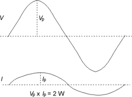 |
| Figure 4.10 Signal power. For a wave, using peak values of
V and
I gives a power that is two times too large. We therefore use RMS values such as
Vp/√2 and
Ip/√2 which will give the correct amount when multiplied |
This is equivalent to using
V and
I quantities that are
Vp/√2 and
Ip/√2, respectively; if you multiply these quantities together you get
VpIp/2, which is the true power in watts. These
Vp/√2 and
Ip/√2 quantities are called
root mean square (RMS) values. We will omit the mathematical theory, but the name comes from the fact that these quantities represent the root of the average (mean) of the square of the peak quantity.
The important point is that if we want to make calculations on the power dissipated by a sinewave, we have to use these RMS quantities. For example, if the peak values of a sinewave are 6
V and 1
A, then the power is not 6
W but only 3
W. This used to be the basis of inflated figures for audio amplifier power outputs, with some manufacturers quoting real RMS power figures and other quoting peak power values (not divided by 2) or even rather imaginary values called
music power.
Note
Note
All of this assumes that the waves of current and voltage are in phase. If they are not, the amount of true power is calculated by multiplying the RMS voltage by the RMS current and multiplying also by the cosine of the phase angle. If the phase angle is 90°, then the power is zero.
Just in case you thought all this was looking quite logical and orderly, the figure of √2 is true only if the waveshape is that of a sinewave, and different factors (called
form factors) have to be used if the waveform is different, as sound waves usually are. This, however, is a worry more for the designers of test equipment than for students of electronics. Fortunately, there are instruments that can measure the RMS values for any form of wave so that we do not need to depend on making peak measurements and performing elaborate mathematics.
Summary
Summary
For sinewave signals, the true power dissipated in a load can be found by multiplying together the RMS values of voltage and current, assuming that these waves are in phase. The RMS value is equal to the peak value for a sinewave divided by √2, a factor of 1.414. For example, the RMS value of a signal which is 10
V peak is 10/1.414
=
7.07
V.
Feedback
A circuit method that is very important for linear amplifiers is called
feedback. Feedback means taking a fraction of the output wave of an amplifier and connecting it to the input. This fed-back signal can be connected so that it either adds to the normal input or subtracts from it (Figure 4.11). If the feedback signal is in phase and so is added to the input wave, this is called
positive feedback, and its action is to increase the apparent gain of the amplifier, reduce its bandwidth, and make the gain figure of the amplifier more sensitive to any changes (such as a small change in the resistance value of a load resistor). If positive feedback is increased to the point where it is enough to provide all the input that the amplifier needs, the result is
oscillation, where the amplifier will provide a wave output without any input.
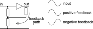 |
| Figure 4.11 Feedback, positive and negative. The feedback signal is a fraction of the output that is added to the input. If this signal is in phase with the input the feedback is positive; if it is in opposite phase (anti-phase) the feedback is negative |
Positive feedback is nowadays seldom used in normal amplifiers, but it is the basis of oscillators that are used to generate signals. Until positive feedback was discovered by Armstrong in 1912, radio signals were generated by rotating machines (alternators) and this limited the frequency of signals that could be used. When active devices are used in an oscillating circuit, the range of frequencies that can be generated is limited mainly by the design of the active components, so that it became easy to generate signals at frequencies of 1
MHz and more. Originally, Armstrong's positive feedback was also used to increase the gain of primitive radio receivers, but this type of use was abandoned in the 1930s because of the interference that was caused when users trying to hear a remote station would cause the radio to oscillate and radiate their own signals.
Negative feedback uses feedback signals that are in opposite phase to the input, and it reduces overall gain. It also increases bandwidth, reduces non-linear behavior, and makes the gain of the amplifier less sensitive to changes in the components. This has made it a standard method that is used by circuit designers who need particularly linear response, stability, and wide bandwidth. It is particularly applicable to opamps (see Chapter 3) and it allows the gain of an amplifier to be set by the ratio of two resistors rather than from elaborate calculations using figures that may not be particularly reliable.
Note
Summary
Note
Negative feedback can reduce some types of distortion, but it does not reduce slew-rate distortion, and can actually cause slew-rate distortion to increase.
Summary
Signal feedback is extensively used in electronics circuits to modify circuit action. If the gain of an amplifier is more than unity, feeding back a portion of the output in phase to the input will increase gain, reduce linearity, and make the amplifier unstable, causing oscillation if the feedback is sufficient. Negative feedback will reduce gain, increase linearity, and make the amplifier more stable, provided the phase of the feedback signal remains at 180°. The performance of a negative-feedback amplifier is determined more by the passive components than by the active components.
Oscillators and Multipliers
An oscillator is a circuit that is designed to generate wave signals from a steady voltage supply, with no wave input. Any oscillator can be thought of as an amplifier with positive feedback and some type of circuit to determine the frequency. If this frequency-determining circuit is a resonant circuit the oscillator is a
tuned oscillator and it will generate sinewaves, or at least waves that are close to a sinewave shape. Other circuits can be used that will cause the oscillator to generate a square or pulse waveform; these are
untuned or
aperiodic oscillators. Oscillators can also be designed so that their oscillating frequency can be varied when a steady voltage input is changed, and this type of oscillator is called a voltage-controlled oscillator (VCO).
A tuned circuit can also be used as a
frequency multiplier. Suppose, for example, that an input signal at 1
MHz is applied to an amplifier which is not linear. The effect of the non-linearity is to change the waveshape, and this means that the signal will now contain other frequencies that are multiples of the original. In this example, the output of the amplifier will contain the 1
MHz signals along with others at 2
MHz, 3
MHz, 4
MHz, and so on. If the output stage is tuned to 2
MHz, this will become the predominant signal at the output, so that the effect of this stage is of a frequency-doubler, converting a 1
MHz signal into a 2
MHz signal.
..................Content has been hidden....................
You can't read the all page of ebook, please click here login for view all page.