7. Collection and Analysis of Rate Data
You can observe a lot just by watching.
Yogi Berra, New York Yankees
7.1 The Algorithm for Data Analysis
For batch systems, the usual procedure is to collect concentration-time data, which we then use to determine the rate law. Table 7-1 gives the seven-step procedure we will emphasize in analyzing reaction engineering data.
Data for homogeneous reactions is most often obtained in a batch reactor. After postulating a rate law in Step 1 and combining it with a mole balance in Step 2, we next use any or all of the methods in Step 5 to process the data and arrive at the reaction orders and specific reaction-rate constants.
Analysis of heterogeneous reactions is shown in Step 6. For gas-solid heterogeneous reactions, we need to have an understanding of the reaction and possible mechanisms in order to postulate the rate law in Step 6B. After studying Chapter 10 on heterogeneous reactions, one will be able to postulate different rate laws and then use Polymath nonlinear regression to choose the “best” rate-law and reaction-rate-law parameters (see Example 10-3 on page 452).
The procedure we should use to delineate the rate law and rate-law parameters is given in Table 7-1.
A. Power-law models for homogeneous reactions
B. Langmuir-Hinshelwood models for heterogeneous reactions
2. Select reactor type and corresponding mole balance.
A. If batch reactor (Section 7.2), use mole balance on Reactant A
B. If differential PBR (Section 7.6), use mole balance on Product P (A → P)
3. Process your data in terms of the measured variable (e.g., NA, CA, or PA). If necessary, rewrite your mole balance in terms of the measured variable (e.g., PA).
4. Look for simplifications. For example, if one of the reactants is in excess, assume its concentration is constant. If the gas-phase mole fraction of reactant A is small, set ε ≈ 0.
5. For a batch reactor, calculate –rA as a function of concentration CA to determine the reaction order.
A. Differential analysis (Section 7.4)
Combine the mole balance (TE7-1.1) and power law model (TE7-1.3)
and then take the natural log
(1) Find ![]() from CA versus t data by either the
from CA versus t data by either the
(a) Graphical differential
(b) Finite differential method or
(c) Polynomial fit
(2) Either plot ![]() versus ln CA to find reaction order α, which is the slope of the line fit to the data or
versus ln CA to find reaction order α, which is the slope of the line fit to the data or
(3) Use nonlinear regression to find α and k simultaneously
B. Integral method (Section 7.3)
For ![]() , the combined mole balance and rate law is
, the combined mole balance and rate law is
Guess α and integrate Equation (TE7-1.4). Rearrange your equation to obtain the appropriate function of CA, which when plotted as a function of time should be linear. If it is linear, then the guessed value of α is correct and the slope is the specific reaction rate, k. If it is not linear, guess again for α. If you guess α = 0, 1, and 2, and none of these orders fit the data, proceed to nonlinear regression.
C. Nonlinear regression (Polymath) (Section 7.5):
Integrate Equation (TE7-1.4) to obtain
Use Polymath regression to find α and k. A Polymath tutorial on regression with screen shots is shown in the Chapter 7 Summary Notes on the CRE Web site, www.umich.edu/~elements/5e/index.html.
6. For differential PBR, calculate ![]() as a function of CA or PA (Section 7.6)
as a function of CA or PA (Section 7.6)
A. Calculate ![]() as a function of reactant concentration, CA or partial pressure PA.
as a function of reactant concentration, CA or partial pressure PA.
B. Choose a model (see Chapter 10), e.g.,

C. Use nonlinear regression to find the best model and model parameters. See example on the CRE Web site Summary Notes for Chapter 10, using data from heterogeneous catalysis.
7. Analyze your rate law model for “goodness of fit.” Calculate a correlation coefficient.
TABLE 7-1 STEPS IN ANALYZING RATE DATA
7.2 Determining the Reaction Order for Each of Two Reactants Using the Method of Excess
Batch reactors are used primarily to determine rate-law parameters for homogeneous reactions. This determination is usually achieved by measuring concentration as a function of time and then using either the integral, differential, or nonlinear regression method of data analysis to determine the reaction order, α, and specific reaction-rate constant, k. If some reaction parameter other than concentration is monitored, such as pressure, the mole balance must be rewritten in terms of the measured variable (e.g., pressure, as shown in the example in Solved Problems on the CRE Web site).
Process data in terms of the measured variable.
When a reaction is irreversible, it is possible in many cases to determine the reaction order α and the specific rate constant by either nonlinear regression or by numerically differentiating concentration versus time data. This latter method is most applicable when reaction conditions are such that the rate is essentially a function of the concentration of only one reactant; for example, if, for the decomposition reaction
A → Products
Assume that the rate law is of the form ![]() .
.
then the differential method may be used.
However, by utilizing the method of excess, it is also possible to determine the relationship between –rA and the concentration of other reactants. That is, for the irreversible reaction
A + B → Products
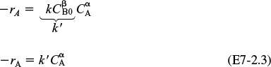
with the rate law
where α and β are both unknown, the reaction could first be run in an excess of B so that CB remains essentially unchanged during the course of the reaction (i.e., CB ≈ CB0) and
where
Method of excess
After determining α, the reaction is carried out in an excess of A, for which the rate law is approximated as
where ![]()
Once α and β are determined, kA can be calculated from the measurement of –rA at known concentrations of A and B
Both α and β can be determined by using the method of excess, coupled with a differential analysis of data for batch systems.
7.3 Integral Method
The integral method is the quickest method to use to determine the rate law if the order turns out to zero, first, or second order. In the integral method, we guess the reaction order, α, in the combined batch reactor mole balance and rate law equation
The integral method uses a trial-and-error procedure to find the reaction order.
and integrate the differential equation to obtain the concentration as a function of time. If the order we assume is correct, the appropriate plot (determined from this integration) of the concentration-time data should be linear. The integral method is used most often when the reaction order is known and it is desired to evaluate the specific reaction rate constant at different temperatures to determine the activation energy.
In the integral method of analysis of rate data, we are looking for the appropriate function of concentration corresponding to a particular rate law that is linear with time. You should be thoroughly familiar with the methods of obtaining these linear plots for reactions of zero, first, and second order.
For the reaction
A → Products
carried out in a constant-volume batch reactor, the mole balance is
It is important to know how to generate linear plots of functions of CA versus t for zero-, first-, and second-order reactions.
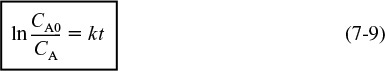
For a zero-order reaction, rA = –k, and the combined rate law and mole balance is
Integrating with CA = CA0 at t = 0, we have
Zero order
A plot of the concentration of A as a function of time will be linear (Figure 7-1) with slope (–k) for a zero-order reaction carried out in a constant-volume batch reactor.
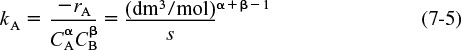
If the reaction is first order (Figure 7-2), integration of the combined mole balance and the rate law
with the limit CA = CA0 at t = 0 gives
First order
Consequently, we see that the slope of a plot of [ln(CA0/CA)] as a function of time is linear with slope k.
If the reaction is second order (Figure 7-3), then


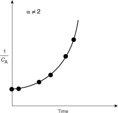
Integrating, with CA = CA0 initially (i.e., t = 0), yields
Second order
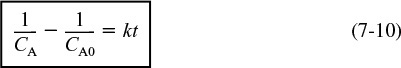
We see that for a second-order reaction a plot of (1/CA) as a function of time should be linear with slope k.
In Figures 7-1, 7-2, and 7-3, we saw that when we plotted the appropriate function of concentration (i.e., CA, ln CA, or 1/CA) versus time, the plots were linear, and we concluded that the reactions were zero, first, or second order, respectively. However, if the plots of concentration data versus time had turned out not to be linear, such as shown in Figure 7-4, we would say that the proposed reaction order did not fit the data. In the case of Figure 7-4, we would conclude that the reaction is not second order. After finding that the integral method for first, second, and third orders do not fit the data, one should use one of the other methods discussed in Table 7-1.
The idea is to arrange the data so that a linear relationship is obtained.
It is important to restate that, given a reaction-rate law, you should be able to quickly choose the appropriate function of concentration or conversion that yields a straight line when plotted against time or space time. The goodnessof-fit of such a line may be assessed statistically by calculating the linear correlation coefficient, r2, which should be as close to 1 as possible. The value of r2 is given in the output of Polymath’s nonlinear regression.
Example 7–1 Integral Method of CRE Data Analysis
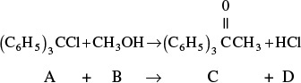
The liquid-phase reaction
Trityl (A) + Methanol (B) → Products (C)
was carried out in a batch reactor at 25°C in a solution of benzene and pyridine in an excess of methanol (![]() ). (We need to point out that this batch reactor was purchased at the Sunday market in Riça, Jofostan.) Pyridine reacts with HCl, which then precipitates as pyridine hydro-chloride thereby making the reaction irreversible. The reaction is first order in methanol. The concentration of triphenyl methyl chloride (A) was measured as a function of time and is shown below
). (We need to point out that this batch reactor was purchased at the Sunday market in Riça, Jofostan.) Pyridine reacts with HCl, which then precipitates as pyridine hydro-chloride thereby making the reaction irreversible. The reaction is first order in methanol. The concentration of triphenyl methyl chloride (A) was measured as a function of time and is shown below

Use the integral method to confirm that the reaction is second order with regard to triphenyl methyl chloride
Solution
We use the power-law model, Equation (7-2), along with information from the problem statement that the reaction is first order in methanol, (B), i.e., β = 1 to obtain
Excess methanol: The initial concentration of methanol (B) is 10 times that of trityl (A), so even if all A were consumed, 90% of B remains. Consequently, we will take the concentration of B as a constant and combine it with k to form
where k′ is the pseudo rate constant k′ = kCB0 and k is the true rate constant. Substituting α = 2 and combining with the mole balance on a batch reactor, we obtain
Integrating with CA = CA0 at t = 0
Rearranging
We see that if the reaction is indeed second order then a plot of (1/CA) versus t should be linear. Using the data in Table E7-1.1, we calculate (1/CA) to construct Table E7-1.2.
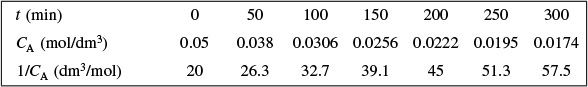
In a graphical solution, the data in Table E7-1.2 can be used to construct a plot of 1/CA as a function of t, which will yield the specific reaction rate k′. This plot is shown in Figure E7-1.1. Again, Excel or Polymath could be used to find k′ from the data in Table E7-1.2. The slope of the line is the specific reaction rate k′.

We see from the Excel analysis and plot that the slope of the line is 0.12 dm3/mol · min.
We now use Equation (E7-1.6), along with the initial concentration of methanol, to find the true rate constant, k.
The rate law is
We note that the integral method tends to smooth the data.
Analysis: In this example, the reaction orders are known so that the integral method can be used to (1) verify the reaction is second order in trityl and (2) to find the specific pseudo reaction rate k′ = kCB0 for the case of excess methanol (B). Knowing k′ and CB0, we can then find the true rate constant k.
7.4 Differential Method of Analysis
To outline the procedure used in the differential method of analysis, we consider a reaction carried out isothermally in a constant-volume batch reactor and the concentration of A, recorded as a function of time. By combining the mole balance with the rate law given by Equation (7-1), we obtain
Constant-volume batch reactor
After taking the natural logarithm of both sides of Equation (5-6)
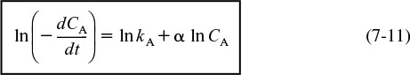
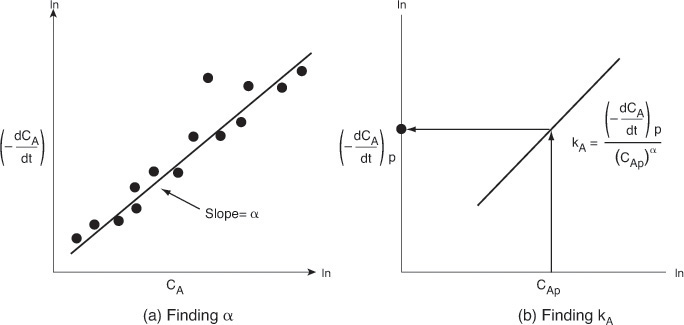
observe that the slope of a plot of [ln(–dCA/dt)] as a function of (ln CA) is the reaction order, α (see Figure 7-5).
Plot ![]() versus ln CA to find α and kA
versus ln CA to find α and kA
Figure 7-5(a) shows a plot of [–(dCA/dt)] versus [CA] on log-log paper (or use Excel to make the plot) where the slope is equal to the reaction order α. The specific reaction rate, kA, can be found by first choosing a concentration in the plot, say CAp, and then finding the corresponding value of [–(dCA/dt)p] on the line, as shown in Figure 7-5(b). The concentration chosen, CAp, to find the derivative at CAp, need not be a data point, it just needs to be on the line. After raising CAp to the power α, we divide it into [–(dCA/dt)p] to determine kA

To obtain the derivative (–dCA/dt) used in this plot, we must differentiate the concentration-time data either numerically or graphically. Three methods to determine the derivative from data giving the concentration as a function of time are
• Graphical differentiation
• Numerical differentiation formulas
• Differentiation of a polynomial fit to the data
Methods for finding ![]() from concentration-time data
from concentration-time data
We shall only discuss the graphical and numerical methods.
7.4.1 Graphical Differentiation Method
This method is very old (from slide rule days–“What’s a slide rule, Grandfather?”), when compared with the numerous software packages. So why do we use it? Because with this method, disparities in the data are easily seen. Consequently, it is advantageous to use this technique to analyze the data before planning the next set of experiments. As explained in Appendix A.2, the graphical method involves plotting (–ΔCA/Δt) as a function of t and then using equal-area differentiation to obtain (–dCA/dt). An illustrative example is also given in Appendix A.2.

See Appendix A.2.
In addition to the graphical technique used to differentiate the data, two other methods are commonly used: differentiation formulas and polynomial fitting.
7.4.2 Numerical Method
Numerical differentiation formulas can be used when the data points in the independent variable are equally spaced, such as t1–t0 = t2–t1 = Δt.
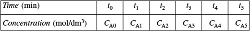
The three-point differentiation formulas1 shown in Table 7-3 can be used to calculate dCA/dt.
1 B. Carnahan, H. A. Luther, and J. O. Wilkes, Applied Numerical Methods (New York: Wiley, 1969), p. 129.
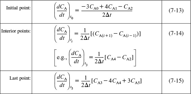
Equations (7-13) and (7-15) are used for the first and last data points, respectively, while Equation (7-14) is used for all intermediate data points (see Step 6A.1a in Example 7-2).
7.4.3 Finding the Rate-Law Parameters
Now, using either the graphical method, differentiation formulas, or the polynomial derivative, the following table can be set up.
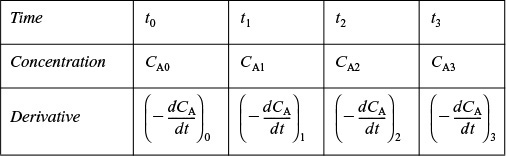
The reaction order can now be found from a plot of ln(–dCA/dt) as a function of ln CA, as shown in Figure 7-5(a), since

Before solving the following example problems, review the steps to determine the reaction-rate law from a set of data points (Table 7-1).
Example 7–2 Determining the Rate Law
The reaction of triphenyl methyl chloride (trityl) (A) and methanol (B) discussed in Example 7-1 is now analyzed using the differential method.
The concentration-time data in Table E7-2.1 was obtained in a batch reactor.

The initial concentration of methanol was 0.5 mol/dm3
Part (1) Determine the reaction order with respect to triphenyl methyl chloride.
Part (2) In a separate set of experiments, the reaction order wrt methanol was found to be first order. Determine the specific reaction-rate constant.
Solution
Part (1) Find the reaction order with respect to trityl.
Step 1 Postulate a rate law.
Step 2 Process your data in terms of the measured variable, which in this case is CA.
Step 3 Look for simplifications. Because the concentration of methanol is 10 times the initial concentration of triphenyl methyl chloride, its concentration is essentially constant
Substituting for CB in Equation (E7-2.1)
Step 4 Apply the CRE algorithm.
Mole Balance
Rate Law:
Stoichiometry: Liquid V = V0
![]()

Combine: Mole balance, rate law, and stoichiometry
Evaluate: Taking the natural log of both sides of Equation (E7-2.5)
The slope of a plot of ln ![]() versus ln CA will yield the reaction order α with respect to triphenyl methyl chloride (A).
versus ln CA will yield the reaction order α with respect to triphenyl methyl chloride (A).
Step 5 Find ![]() as a function of CA from concentration-time data.
as a function of CA from concentration-time data.
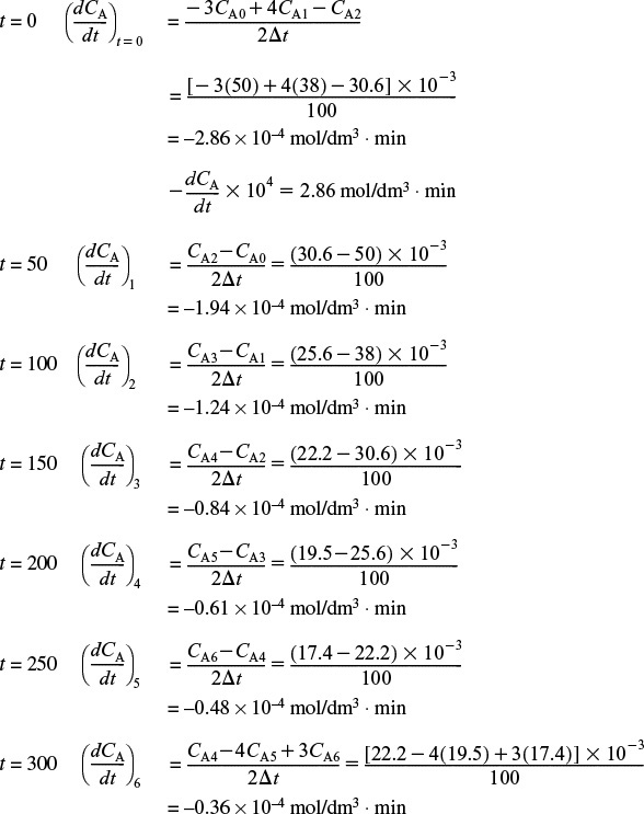
Step 5A.1a Graphical Method. We now show how to construct Table E7-2.2. The derivative (–dCA/dt) is determined by calculating and plotting (–ΔCA/Δt) as a function of time, t, and then using the equal-area differentiation technique (Appendix A.2) to determine (–dCA/dt) as a function of CA. First, we calculate the ratio (–ΔCA/Δt) from the first two columns of Table E7-2.2; the result is written in the third column.
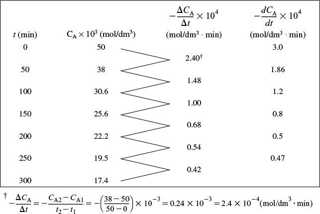
Next, we use Table E7-2.2 to plot the third column as a function of the first column in Figure E7-1.1 [i.e., (–ΔCA/Δt) versus t]. Using equal-area differentiation, the value of (–dCA/dt) is read off the figure (represented by the arrows); then it is used to complete the fourth column of Table E7-2.2.

The results to find (–dCA/dt) at each time, t, and concentration, CA, are summarized in Table E7-2.3.
Step 6A.1a Finite Difference Method. We now show how to calculate (dCA/dt) using the finite difference formulas [i.e., Equations (7-13) through (7-15)].
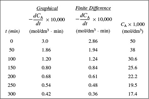
We now enter the above values for (–dCA/dt) in Table E7-2.3 and use Table 7-2.2 to plot columns 2 and 3 ![]() as a function of column 4 (CA×1,000) on log-1og paper, as shown in Figure E7-2.2. We could also substitute the parameter values in Table E7-2.3 into Excel to find α and k′. Note that most of the points for both methods fall virtually on top of one another. This table is, in a way, redundant because it is not necessary to always find (–dCAdt) by both techniques, graphical and finite difference.
as a function of column 4 (CA×1,000) on log-1og paper, as shown in Figure E7-2.2. We could also substitute the parameter values in Table E7-2.3 into Excel to find α and k′. Note that most of the points for both methods fall virtually on top of one another. This table is, in a way, redundant because it is not necessary to always find (–dCAdt) by both techniques, graphical and finite difference.

From Figure E7-2.2, we found the slope to be 1.99, so that the reaction is said to be second order (α = 2.0) with respect to triphenyl methyl chloride. To evaluate k′, we can evaluate the derivative in Figure E7-2.2 at CAp = 20 × 10–3mol/dm3, which is
then

As will be shown in Section 7-5, we could also use nonlinear regression on Equation (E7-1.5) to find k′
The Excel graph shown in Figure E7-2.2 gives α = 1.99 and k′ = 0.13 dm3/mol · min. We now set α = 2 and regress again to find k′ = 0.122 dm3/mol · min.
ODE Regression. There are techniques and software becoming available whereby an ODE solver can be combined with a regression program to solve differential equations, such as
to find kA and α from concentration—time data.
Part (2) The reaction was said to be first order with respect to methanol. β = 1.
Assuming CB0 is constant at 0.5 mol/dm3 and solving for k yields2
2 M. Hoepfner and D. K. Roper, “Describing Temperature Increases in Plasmon-Resonant Nanoparticle Systems,” Journal of Thermal Analysis and Calorimetry, 98(1), (2009), pp. 197-202.

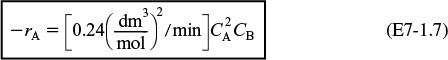
The rate law is
Analysis: In this example, the differential method of data analysis was used to find the reaction order with respect to trityl (α = 1.99) and the pseudo rate constant (k′ = 0.125 (dm3/mol)/min). The reaction order was rounded up to α = 2 and the data was regressed again to obtain k′ = 0.122 (dm3/mol)/min, again knowing k′ and CB0, and the true rate constant is k = 0.244 (dm3/mol)2/min.
By comparing the methods of analysis of the rate data presented in Examples 7-1 and 7-2, we note that the differential method tends to accentuate the uncertainties in the data, while the integral method tends to smooth the data, thereby disguising the uncertainties in it. In most analyses, it is imperative that the engineer know the limits and uncertainties in the data. This prior knowledge is necessary to provide for a safety factor when scaling up a process from laboratory experiments to design either a pilot plant or full-scale industrial plant.
Integral method normally used to find k when order is known
7.5 Nonlinear Regression
In nonlinear regression analysis, we search for those parameter values that minimize the sum of the squares of the differences between the measured values and the calculated values for all the data points. Not only can nonlinear regression find the best estimates of parameter values, it can also be used to discriminate between different rate-law models, such as the LangmuirHinshelwood models discussed in Chapter 10. Many software programs are available to find these parameter values so that all one has to do is enter the data. The Polymath software will be used to illustrate this technique. In order to carry out the search efficiently, in some cases one has to enter initial estimates of the parameter values close to the actual values. These estimates can be obtained using the linear-least-squares technique discussed on the CRE Web site Professional Reference Shelf R7.3.
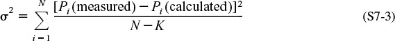
We will now apply nonlinear regression to reaction-rate data to determine the rate-law parameters. Here, we make initial estimates of the parameter values (e.g., reaction order, specific rate constant) in order to calculate the concentration for each data point, Cic, obtained by solving an integrated form of the combined mole balance and rate law. We then compare the measured concentration at that point, Cim, with the calculated value, Cic, for the parameter values chosen. We make this comparison by calculating the sum of the squares of the differences at each point Σ(Cim – Cic)2. We then continue to choose new parameter values and search for those values of the rate law that will minimize the sum of the squared differences of the measured concentrations, Cim, and the calculated concentrations values, Cic. That is, we want to find the rate-law parameters for which the sum of all data points Σ(Cim–Cic)2 is a minimum. If we carried out N experiments, we would want to find the parameter values (e.g., E, activation energy, reaction orders) that minimize the quantity
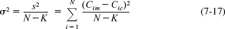
where

One notes that if we minimize s2 in Equation (7-17), we minimize σ2.
To illustrate this technique, let’s consider the reaction
for which we want to learn the reaction order, α, and the specific reaction rate, k,
The reaction rate will be measured at a number of different concentrations. We now choose values of k and α, and calculate the rate of reaction (Cic) at each concentration at which an experimental point was taken. We then subtract the calculated value (Cic) from the measured value (Cim), square the result, and sum the squares for all the runs for the values of k and α that we have chosen.
This procedure is continued by further varying α and k until we find those values of k and α that minimize the sum of the squares. Many well-known searching techniques are available to obtain the minimum value ![]() .3 Figure 7-6 shows a hypothetical plot of the sum of the squares as a function of the parameters α and k:
.3 Figure 7-6 shows a hypothetical plot of the sum of the squares as a function of the parameters α and k:
3 (a) B. Carnahan and J. O. Wilkes, Digital Computing and Numerical Methods (New York: Wiley, 1973), p. 405. (b) D. J. Wilde and C. S. Beightler, Foundations of Optimization, 2nd ed. (Upper Saddle River, NJ: Prentice Hall, 1979). (c) D. Miller and M. Frenklach, Int. J. Chem. Kinet., 15 (1983), p. 677.
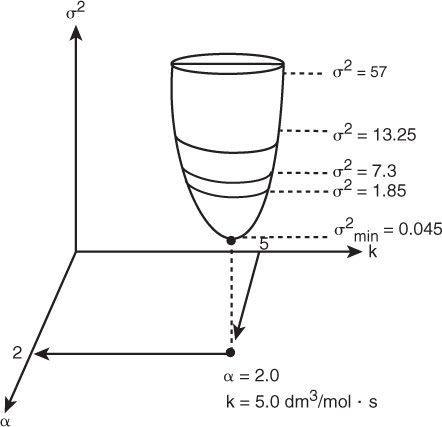
Look at the top circle. We see that there are many combinations of α and k (e.g., α = 2.2, k = 4.8 or α = 1.8, k = 5.3) that will give a value of σ2 = 57. The same is true for σ2 = 1.85. We need to find the combination of α and k that gives the lowest value of σ2.
In searching to find the parameter values that give the minimum of the sum of squares σ2, one can use a number of optimization techniques or software packages. The searching procedure begins by guessing parameter values and then calculating (Cim–Cic) and then σ2 for these values. Next, a few sets of parameters are chosen around the initial guess, and σ2 is calculated for these sets as well. The search technique looks for the smallest value of σ2 in the vicinity of the initial guess and then proceeds along a trajectory in the direction of decreasing σ2 to choose different parameter values and determine the corresponding σ2. The trajectory is continually adjusted so as to always proceed in the direction of decreasing σ2 until the minimum value of σ2 is reached. For example, in Figure 7-6 the search technique keeps choosing combinations of α and k until a minimum value of σ2 = 0.045 (mol/dm3)2 is reached. The combination that gives that minimum is α = 2 and k = 5.0 dm3/mol·min as shown in Figure 7-6. If the equations are highly nonlinear, the initial guesses of α and k are very important.

A number of software packages are available to carry out the procedure to determine the best estimates of the parameter values and the corresponding confidence limits. All we have to do is to enter the experimental values into the computer, specify the model, enter the initial guesses of the parameters, and then push the “compute” button, and the best estimates of the parameter values along with 95% confidence limits appear. If the confidence limits for a given parameter are larger than the parameter itself, the parameter is probably not significant and should be dropped from the model. After the appropriate model parameters are eliminated, the software is run again to determine the best fit with the new model equation.
Concentration-Time Data. We will now use nonlinear regression to determine the rate-law parameters from concentration-time data obtained in batch experiments. We recall that the combined rate-law stoichiometry mole balance for a constant-volume batch reactor is
We now integrate Equation (7-6) to give
Rearranging to obtain the concentration as a function of time, we obtain
Now we could use either Polymath or MATLAB to find the values of α and k that would minimize the sum of squares of the differences between the measured concentrations, CAim, and calculated concentrations, CAic. That is, for N data points,

we want the values of α and k that will make s2 a minimum.
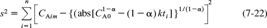
If Polymath is used, one should use the absolute value for the term in brackets in Equation (7-16), that is,
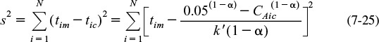
Another, and perhaps easier, way to solve for the parameter values is to use time rather than concentrations, rearranging Equation (7-20) to get

That is, we find the values of k and α that minimize

Finally, a discussion of weighted least squares as applied to a first-order reaction is provided in the Professional Reference Shelf R7.5 on the CRE Web site.
Example 7–3 Use of Regression to Find the Rate-Law Parameters
We shall use the reaction and data in Examples E7-1 and E7-2 to illustrate how to use regression to find α and k′.
The Polymath regression program is included on the CRE Web site. Recalling Equation (E5-1.5)
and integrating with the initial condition when t = 0 and CA = CA0 for α≠1.0

Given or assuming k′ and α, Equation (7-2.5) can be solved to calculate the time t to reach a concentration CA or we could calculate the concentration CA at time t. We can proceed two ways from this point, both of which will give the same result. We can search for the combination α and k that minimizes [σ2 = ∑(tim–tic)2], or we could solve Equation (E7-4.3) for CA and find α and k that minimize [σ2 = ∑(CAim–CAic)2]. We shall choose the former. So, substituting for the initial concentration CA0 = 0.05 mol/dm3 into Equation (E7-3.1)
A brief tutorial on how to input data in Polymath is given in the Polymath link in the Summary Notes on the CRE Web site for Chapter 7. The Polymath tutorial on the CRE Web site shows screen shots of how to enter the raw data in Table E7-2.1 and how to carry out a nonlinear regression on Equation (E7-3.2). For CA0 = 0.05 mol/dm3, that is, Equation (E7-3.1) becomes

We want to minimize s2 to give α and k′.
The result of the first and second Polymath regressions are shown in Tables E7-3.1 and E7-3.2.


The first regression gives α = 2.04, as shown in Table E7-3.1. We shall round off α to make the reaction second order, (i.e., α = 2.00). Now having fixed α at 2.0, we must do another regression (cf. Table E7-3.2) on k′ because the k′ given in Table E7-3.1 is for α = 2.04. We now regress the equation
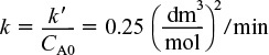
The second regression gives k′ = 0.125 dm3/mol·min. We now calculate k
Analysis: In this example, we showed how to use nonlinear regression to find k′ and α. The first regression gave α = 2.04, which we rounded to 2.00 and then regressed again for the best value of k′ for α = 2.0, which was k′ = 0.125(dm3/mol)/min giving a value of the true specific reaction rate of k = 0.25(mol/dm3)2/min. We note that the reaction order is the same as that in Examples 7-1 and 7-2; however, the value of k is about 8% larger. The r2 and other statistics are in Polymath’s output.
Model Discrimination. One can also determine which model or equation best fits the experimental data by comparing the sums of the squares for each model and then choosing the equation with a smaller sum of squares and/or carrying out an F-test. Alternatively, we can compare the residual plots for each model. These plots show the error associated with each data point, and one looks to see if the error is randomly distributed or if there is a trend in the error. When the error is randomly distributed, this is an additional indication that the correct rate law has been chosen. An example of model discrimination using nonlinear regression is given in Chapter 10.
7.6 Reaction-Rate Data from Differential Reactors
Data acquisition using the method of initial rates and a differential reactor is similar in that the rate of reaction is determined for a specified number of predetermined initial or entering reactant concentrations. A differential reactor (PBR) is normally used to determine the rate of reaction as a function of either concentration or partial pressure. It consists of a tube containing a very small amount of catalyst, usually arranged in the form of a thin wafer or disk. A typical arrangement is shown schematically in Figure 7-7. The criterion for a reactor being differential is that the conversion of the reactants in the bed is extremely small, as is the change in temperature and reactant concentration through the bed. As a result, the reactant concentration through the reactor is essentially constant and approximately equal to the inlet concentration. That is, the reactor is considered to be gradientless,4 and the reaction rate is considered spatially uniform within the bed.
4 B. Anderson, ed., Experimental Methods in Catalytic Research (San Diego, CA: Academic Press, 1976).
Most commonly used catalytic reactor to obtain experimental data
The differential reactor is relatively easy to construct at a low cost. Owing to the low conversion achieved in this reactor, the heat release per unit volume will be small (or can be made small by diluting the bed with inert solids) so that the reactor operates essentially in an isothermal manner. When operating this reactor, precautions must be taken so that the reactant gas or liquid does not bypass or channel through the packed catalyst, but instead flows uniformly across the catalyst. If the catalyst under investigation decays rapidly, the differential reactor is not a good choice because the reaction-rate parameters at the start of a run will be different from those at the end of the run. In some cases, sampling and analysis of the product stream may be difficult for small conversions in multicomponent systems.


Limitations of the differential reactor
For the reaction of species A going to product (P)
A → P
the volumetric flow rate through the catalyst bed is monitored, as are the entering and exiting concentrations (Figure 7-9). Therefore, if the weight of catalyst, ΔW, is known, the rate of reaction per unit mass of catalyst, ![]() , can be calculated. Since the differential reactor is assumed to be gradientless, the design equation will be similar to the CSTR design equation. A steady-state mole balance on reactant A gives
, can be calculated. Since the differential reactor is assumed to be gradientless, the design equation will be similar to the CSTR design equation. A steady-state mole balance on reactant A gives
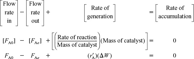
The subscript e refers to the exit of the reactor. Solving for ![]() , we have
, we have
The mole balance equation can also be written in terms of concentration
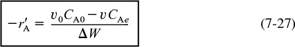
Differential reactor design equation
or in terms of conversion or product flow rate FP
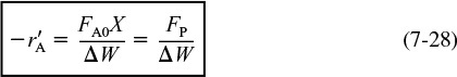
The term FA0X gives the rate of formation of product, FP, when the stoichiometric coefficients of A and of P are identical. Adjustments to Equation (7-28) must be made when this is not the case.
For constant volumetric flow, Equation (7-28) reduces to
Consequently, we see that the reaction rate, ![]() , can be determined by measuring the product concentration, CP.
, can be determined by measuring the product concentration, CP.
By using very little catalyst and large volumetric flow rates, the concentration difference, (CA0 – CAe), can be made quite small. The rate of reaction determined from Equation (7-29) can be obtained as a function of the reactant concentration in the catalyst bed, CAb
by varying the inlet concentration. One approximation of the concentration of A within the bed, CAb, would be the arithmetic mean of the inlet and outlet concentrations
However, since very little reaction takes place within the bed, the bed concentration is essentially equal to the inlet concentration
CAb ≈ CA0
so ![]() is a function of CA0
is a function of CA0
As with the method of initial rates (see the CRE Web site, PRS R7.1), various numerical and graphical techniques can be used to determine the appropriate algebraic equation for the rate law. When collecting data for fluid-solid reacting systems, care must be taken that we use high flow rates through the differential reactor and small catalyst particle sizes in order to avoid mass transfer limitations. If data show the reaction to be first order with a low activation energy, say 8 kcal/mol, one should suspect the data are being collected in the mass transfer limited regime. We will expand on mass transfer limitations and how to avoid them in Chapters 10, 14, and 15.

Example 7–4 Using a Differential Reactor to Obtain Catalytic Rate Data
The formation of methane from carbon monoxide and hydrogen using a nickel catalyst was studied by Pursley.5 The reaction
5 J. A. Pursley, “An Investigation of the Reaction between Carbon Monoxide and Hydrogen on a Nickel Catalyst above One Atmosphere,” Ph.D. thesis, University of Michigan.
3H2 + CO → CH4 + H2O
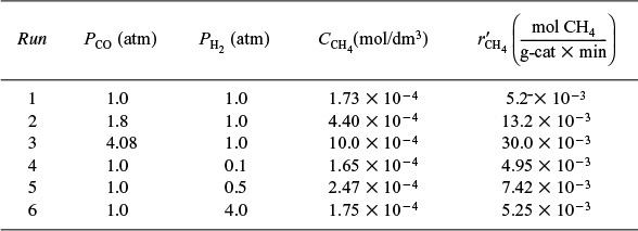
was carried out at 500°F in a differential reactor where the effluent concentration of methane was measured. The raw data is shown in Table E7-4.1.
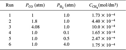
PH2 is constant in Runs 1, 2, 3.
PCO is constant in Runs 4, 5, 6.
The exit volumetric flow rate from a differential packed bed containing 10 g of catalyst was maintained at 300 dm3/min for each run. The partial pressures of H2 and CO were determined at the entrance to the reactor, and the methane concentration was measured at the reactor exit. Determine the rate law and rate law parameters.
(a) Relate the rate of reaction to the exit methane concentration. The reaction-rate law is assumed to be the product of a function of the partial pressure of CO and a function of the partial pressure of H2,
(b) Determine the rate-law dependence on carbon monoxide, using the data generated in part (a). Assume that the functional dependence of ![]() on PCO is of the form
on PCO is of the form
(c) Determine the rate-law dependence on H2. Generate a table of the reaction rate as a function of partial pressures of carbon monoxide and hydrogen.
Solution
(a) Calculate the Rates of Reaction. In this example the product composition, rather than the reactant concentration, is being monitored. The term (![]() ) can be written in terms of the flow rate of methane from the reaction
) can be written in terms of the flow rate of methane from the reaction
Substituting for FCH4 in terms of the volumetric flow rate and the concentration of methane gives
Since υ0, CCH4, and ΔW are known for each run, we can calculate the rate of reaction.
For run 1
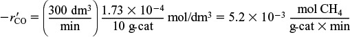
The rate for runs 2 through 6 can be calculated in a similar manner (Table E7-4.2).
(b) Determining the Rate-Law Dependence in CO. For constant hydrogen concentration (runs 1, 2, and 3), the rate law
can be written as
Taking the natural log of Equation (E7-5.4) gives us
We now plot ln (![]() ) versus lnPCO using runs 1, 2, and 3, for which the H2 concentration is constant, in Figure E7-4.1. We see from the Excel plot that α = 1.22.
) versus lnPCO using runs 1, 2, and 3, for which the H2 concentration is constant, in Figure E7-4.1. We see from the Excel plot that α = 1.22.
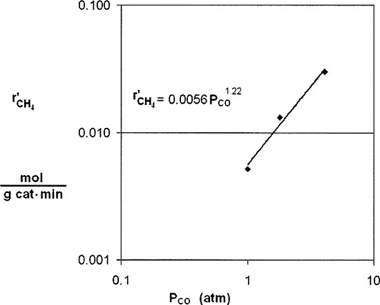
If we had used more data (not given here) we would have found α = 1.
Had we included more points, we would have found that the reaction is essentially first order with α = 1, that is
From the first three data points where the partial pressure of H2 is constant, we see the rate is linear in partial pressure of CO
r′CH4 = k′PCO·g(H2)
Now let’s look at the hydrogen dependence.
(c) Determining the Rate-Law Dependence on H2. From Table E7-4.2 it appears that the dependence of ![]() on PH2 cannot be represented by a power law. Comparing run 4 with run 5 and then run 5 with run 6, we see that the reaction rate first increases with increasing partial pressure of hydrogen, and subsequently decreases with increasing PH2. That is, there appears to be a concentration of hydrogen at which the rate is maximum. One set of rate laws that is consistent with these observations is:
on PH2 cannot be represented by a power law. Comparing run 4 with run 5 and then run 5 with run 6, we see that the reaction rate first increases with increasing partial pressure of hydrogen, and subsequently decreases with increasing PH2. That is, there appears to be a concentration of hydrogen at which the rate is maximum. One set of rate laws that is consistent with these observations is:
1. At low H2 concentrations where ![]() increases as PH2 increases, the rate law may be of the form
increases as PH2 increases, the rate law may be of the form
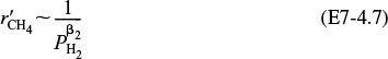
2. At high H2 concentrations where ![]() decreases as PH2 increases, the rate law may be of the form
decreases as PH2 increases, the rate law may be of the form
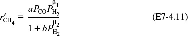
We would like to find one rate law that is consistent with reaction-rate data at both high and low hydrogen concentrations. After we have studied heterogeneous reactions in Chapter 10, we would recognize that Equations (E7-4.6) and (E7-4.7) can be combined into the form

We will see in Chapter 10 that this combination and similar rate laws that have reactant concentrations (or partial pressures) in the numerator and denominator are common in heterogeneous catalysis.
Let’s see if the resulting rate law (E7-4.8) is qualitatively consistent with the rate observed.
1. For condition 1: At low PH2, [b(PH2)β2![]() 1] and Equation (E7-4.8) reduces to
1] and Equation (E7-4.8) reduces to
Equation (E7-4.9) is consistent with the trend in comparing runs 4 and 5.
2. For condition 2: At high PH2, [b(PH2)β2![]() 1] and Equation (E5-5.8) reduces to
1] and Equation (E5-5.8) reduces to

where β2 > β1. Equation (E7-4.10) is consistent with the trends in comparing run 5 and 6.
Combining Equations (E7-4.8) and (E7-4.5)
Typical form of the rate law for heterogeneous catalysis
We now use the Polymath regression program to find the parameter values a, b, β1, β2. The results are shown in Table E7-4.3.
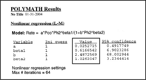
Polymath and Excel regression tutorial are given in the Chapter 7 Summary Notes on the CRE Web site.
The corresponding rate law is
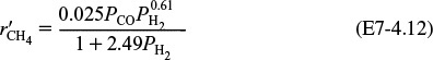
We could use the rate law given by Equation (E7-4.12) as is, but there are only six data points, and we should be concerned about extrapolating the rate law over a wider range of partial pressures. We could take more data, and/or we could carry out a theoretical analysis of the type discussed in Chapter 10 for heterogeneous reactions. If we assume hydrogen undergoes dissociative adsorption on the catalyst surface, we would expect a dependence on the partial pressure of hydrogen to be to the ½ power. Because 0.61 is close to 0.5, we are going to regress the data again, setting β1 = ½ and β2 = 1.0. The results are shown in Table E7-4.4.
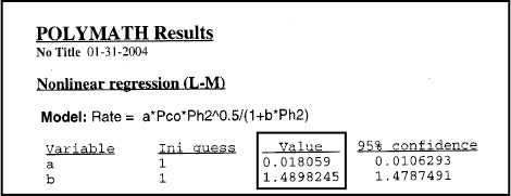
The rate law is now
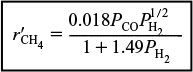
where ![]() is in (mol/g-cat · s) and the partial pressures are in (atm).
is in (mol/g-cat · s) and the partial pressures are in (atm).
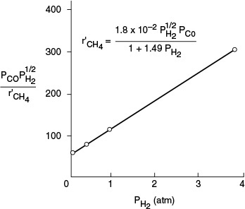
We could also have set β1 = ½ and β2 = 1.0 and rearranged Equation (E7-4.11) in the form

Linearizing the rate law to determine the rate law parameters
A plot of ![]() as a function of PH2 should be a straight line with an intercept of 1/a and a slope of b/a. From the plot in Figure E7-4.2, we see that the rate law is indeed consistent with the rate-law data.
as a function of PH2 should be a straight line with an intercept of 1/a and a slope of b/a. From the plot in Figure E7-4.2, we see that the rate law is indeed consistent with the rate-law data.
Analysis: The reaction-rate data in this example were obtained at steady state, and as a result, neither the integral method nor differential method of analysis can be used. One of the purposes of this example is to show how to reason out the form of the rate law and to then use regression to determine the rate-law parameters. Once the parameters were obtained, we showed how to linearize the rate-law [e.g., Equation (E7-4.13) ] to generate a single plot of all the data, Figure (E7-4.2).
G. C. Quarderer, Dow Chemical Co.
So far, this chapter has presented various methods of analyzing rate data. It is just as important to know in which circumstances to use each method as it is to know the mechanics of these methods. In the Expanded Material on the CRE Web site, we give a thumbnail sketch of a heuristic to plan experiments to generate the data necessary for reactor design. However, for a more thorough discussion, the reader is referred to the books and articles by Box and Hunter.6
6 G. E. P. Box, W. G. Hunter, and J. S. Hunter, Statistics for Experimenters: An Introduction to Design, Data Analysis, and Model Building (New York: Wiley, 1978).
Summary
1. Integral method
a. Guess the reaction order and integrate the mole balance equation.
b. Calculate the resulting function of concentration for the data and plot it as a function of time. If the resulting plot is linear, you have probably guessed the correct reaction order.
c. If the plot is not linear, guess another order and repeat the procedure.
2. Differential method for constant-volume systems
a. Plot –ΔCA/Δt as a function of t.
b. Determine –dCA/dt from this plot.
c. Take the ln of both sides of (S7-1) to get
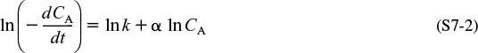
Plot ln(–dCA/dt) versus ln CA. The slope will be the reaction order α. We could use finite-difference formulas or software packages to evaluate (–dCA/dt) as a function of time and concentration.
3. Nonlinear regression: Search for the parameters of the rate law that will minimize the sum of the squares of the difference between the measured rate of reaction and the rate of reaction calculated from the parameter values chosen. For N experimental runs and K parameters to be determined, use Polymath.

Caution: Be sure to avoid a false minimum in σ2 by varying your initial guess.
4. Modeling the differential reactor:
The rate of reaction is calculated from the equation
In calculating the reaction order, α
the concentration of A is evaluated either at the entrance conditions or at a mean value between CA0 and CAe. However, power-law models such as
are not the best way to describe heterogeneous reaction-rate laws. Typically, they take the form
or a similar form, with the reactant partial pressures in the numerator and denominator of the rate law.
CRE Web Site Materials
• Expanded Material
1. Evaluation of Laboratory Reactors
2. Summary of Reactor-Ratings, Gas-liquid, Powdered Catalyst Decaying Catalyst System
3. Experimental Planning
4. Additional Homework Problems
• Learning Resources
1. Summary Notes
2. Interactive Computer Games

B. Reactor Lab (www.reactorlab.net). See Reactor Lab Chapter 7 and P7-3A.
3. Solved Problems
A. Example: Differential Method of Analysis of Pressure- Time Data
B. Example: Integral Method of Analysis of Pressure- Time Data
C. Example: Oxygenating Blood

• Living Example Problems
1. Example 7-3 Use of Regression to Find the Rate Law Parameters
• FAQ (Frequently Asked Questions)—In Updates/FAQ icon section
• Professional Reference Shelf
R7.1. Method of Initial Rates
R7.2. Method of Half Lives
R7.3. Least-Squares Analysis of the Linearized Rate Law
The CRE Web site describes how the rate law
is linearized
ln(–rA) = ln k + α ln CA + β ln CB
and put in the form
Y = a0 + αX1 + βX2
and used to solve for α, β, and k. The etching of a semiconductor, MnO2, is used as an example to illustrate this technique.
R7.4. A Discussion of Weighted Least Squares
For the case when the error in measurement is not constant, we must use a weighted least-squares analysis.
A. Why perform the experiment?
B. Are you choosing the correct parameters?
C. What is the range of your experimental variables?
D. Can you repeat the measurement? (Precision)
E. Milk your data for all it’s worth.
F. We don’t believe an experiment until it’s proven by theory.
G. Tell someone about your result.
R7.6. Evaluation or Laboratory Reactor
Questions and Problems
The subscript to each of the problem numbers indicates the level of difficulty: A, least difficult; D, most difficult.

Questions
Q7-1A
(a) Listen to the audios ![]() on the CRE Web site and pick one and say why it could be eliminated.
on the CRE Web site and pick one and say why it could be eliminated.
(b) Create an original problem based on Chapter 7 material.
(c) Design an experiment for the undergraduate laboratory that demonstrates the principles of chemical reaction engineering and will cost less than $500 in purchased parts to build. (From 1998 AIChE National Student Chapter Competition). Rules are provided on the CRE Web site.
(d) K-12 Experiment. Plant a number of seeds in different pots (corn works well). The plant and soil of each pot will be subjected to different conditions. Measure the height of the plant as a function of time and fertilizer concentration. Other variables might include lighting, pH, and room temperature. (Great grade school or high school science project.)

(a) Revisit Example 7-1. What is the error in assuming the concentration of species B is constant and what limits can you put on the calculated value of k? (I.e., k = 0.24 ±?)
(b) Revisit Example 7-3. Explain why the regression was carried out twice to find k′ and k.
(c) Revisit Example 7-4. Regress the data to fit the rate law
What is the difference in the correlation and sums of squares compared with those given in Example 7-4? Why was it necessary to regress the data twice, once to obtain Table E7-4.3 and once to obtain Table E7-4.4?
P7-2A Download the Interactive Computer Game (ICG) from the CRE Web site. Play the game and then record your performance number for the module that indicates your mastery of the material. Your professor has the key to decode your performance number.
ICM Ecology Performance #_________________________.
P7-3A Go to Professor Herz’s Reactor Lab on the Web at www.reactorlab.net. Do (a) one quiz, or (b) two quizzes from Division 1. When you first enter a lab, you see all input values and can vary them. In a lab, click on the Quiz button in the navigation bar to enter the quiz for that lab. In a quiz, you cannot see some of the input values: you need to find those with “???” hiding the values. In the quiz, perform experiments and analyze your data in order to determine the unknown values. See the bottom of the Example Quiz page at www.reactorlab.net for equations that relate E and k. Click on the “???” next to an input and supply your value. Your answer will be accepted if it is within ±20% of the correct value. Scoring is done with imaginary dollars to emphasize that you should design your experimental study rather than do random experiments. Each time you enter a quiz, new unknown values are assigned. To reenter an unfinished quiz at the same stage you left, click the [i] info button in the Directory for instructions. Turn in copies of your data, your analysis work, and the Budget Report.
P7-4A When arterial blood enters a tissue capillary, it exchanges oxygen and carbon dioxide with its environment, as shown in this diagram.

The kinetics of this deoxygenation of hemoglobin in blood was studied with the aid of a tubular reactor by Nakamura and Staub (J. Physiol., 173, 161).
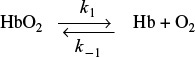
Although this is a reversible reaction, measurements were made in the initial phases of the decomposition so that the reverse reaction could be neglected. Consider a system similar to the one used by Nakamura and Staub: the solution enters a tubular reactor (0.158 cm in diameter) that has oxygen electrodes placed at 5-cm intervals down the tube. The solution flow rate into the reactor is 19.6 cm3/s with CA0 = 2.33 × 10⁻⁶mol/cm3.

(a) Using the method of differential analysis of rate data, determine the reaction order and the forward specific reaction-rate constant k1 for the deoxygenation of hemoglobin.
(b) Repeat using regression.
P7-5B The liquid-phase irreversible reaction
A → B + C
is carried out in a CSTR. To learn the rate law, the volumetric flow rate, υ0, (hence τ = V/υ0) is varied and the effluent concentrations of species A are recorded as a function of the space time τ. Pure A enters the reactor at a concentration of 2 mol/dm3. Steady-state conditions exist when the measurements are recorded.
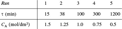
(a) Determine the reaction order and specific reaction-rate constant.
(b) If you were to repeat this experiment to determine the kinetics, what would you do differently? Would you run at a higher, lower, or the same temperature? If you were to take more data, where would you place the measurements (e.g., τ)?
(c) It is believed that the technician may have made a dilution factor-of-10 error in one of the concentration measurements. What do you think? How do your answers compare using regression (Polymath or other software) with those obtained by graphical methods?
Note: All measurements were taken at steady-state conditions.
A → B + C
was carried out in a constant-volume batch reactor where the following concentration measurements were recorded as a function of time.

(a) Use nonlinear least squares (i.e., regression) and one other method to determine the reaction order, α, and the specific reaction rate, k.
(b) Nicolas Bellini wants to know, if you were to take more data, where would you place the points? Why?
(c) Prof. Dr. Sven Köttlov from Jofostan University always asks his students, if you were to repeat this experiment to determine the kinetics, what would you do differently? Would you run at a higher, lower, or the same temperature? Take different data points? Explain.
(d) It is believed that the technician made a dilution error in the concentration measured at 60 min. What do you think? How do your answers compare using regression (Polymath or other software) with those obtained by graphical methods?
P7-7A The following data were reported [from C. N. Hinshelwood and P. J. Ackey, Proc. R. Soc. (Lond)., A115, 215] for a gas-phase constant-volume decomposition of dimethyl ether at 504°C in a batch reactor. Initially, only (CH3)2O was present.
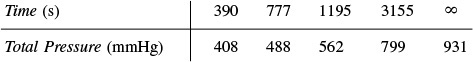
(a) Why do you think the total pressure measurement at t = 0 is missing? Can you estimate it?
(b) Assuming that the reaction
(CH3)2O → CH4 + H2 + CO
is irreversible and goes virtually to completion, determine the reaction order and specific reaction rate k. (Ans.: k = 0.00048 min–1)
(c) What experimental conditions would you suggest if you were to obtain more data?
(d) How would the data and your answers change if the reaction were run at a higher temperature? A lower temperature?
P7-8A In order to study the photochemical decay of aqueous bromine in bright sunlight, a small quantity of liquid bromine was dissolved in water contained in a glass battery jar and placed in direct sunlight. The following data were obtained at 25°C:
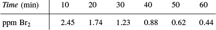
(a) Determine whether the reaction rate is zero, first, or second order in bromine, and calculate the reaction-rate constant in units of your choice.
(b) Assuming identical exposure conditions, calculate the required hourly rate of injection of bromine (in pounds per hour) into a sunlit body of water, 25,000 gal in volume, in order to maintain a sterilizing level of bromine of 1.0 ppm. [Ans.: 0.43 lb/h]
(c) Apply one or more of the six ideas in Preface Table P-4, page xxviii, to this problem.
(Note: ppm = parts of bromine per million parts of brominated water by weight. In dilute aqueous solutions, 1 ppm ≡ 1 milligram per liter.) (From California Professional Engineers’ Exam.)
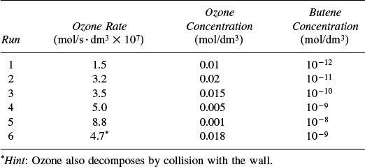
P7-9C The reactions of ozone were studied in the presence of alkenes [from R. Atkinson et al., Int. J. Chem. Kinet., 15(8), 721 (1983) ]. The data in Table P7-9C are for one of the alkenes studied, cis-2-butene. The reaction was carried out isothermally at 297 K. Determine the rate law and the values of the rate-law parameters.
P7-10A Tests were run on a small experimental reactor used for decomposing nitrogen oxides in an automobile exhaust stream. In one series of tests, a nitrogen stream containing various concentrations of NO2 was fed to a reactor, and the kinetic data obtained are shown in Figure P7-10A. Each point represents one complete run. The reactor operates essentially as an isothermal backmix reactor (CSTR). What can you deduce about the apparent order of the reaction over the temperature range studied?
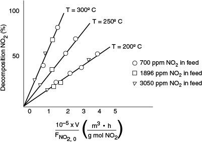
The plot gives the fractional decomposition of NO2 fed versus the ratio of reactor volume V (in cm3) to the NO2 feed rate, FNO2,0 (g mol/h), at different feed concentrations of NO2 (in parts per million by weight). Determine as many rate law parameters as you can.
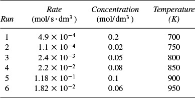
P7-11A The thermal decomposition of isopropyl isocyanate was studied in a differential packed-bed reactor. From the data in Table P7-11A, determine the reaction-rate-law parameters.
• Additional Homework Problems are on the CRE Web site
New Problems on the Web
CDP7-New From time to time, new problems relating Chapter 7 material to everyday interests or emerging technologies will be placed on the Web. Solutions to these problems can be obtained by emailing the author. Also, one can go to the Web site, nebula.rowan.edu:82/home.asp, and work the home problem specific to this chapter.

Green Engineering

Supplementary Reading
1. A wide variety of techniques for measuring the concentrations of the reacting species may or may not be found in
BURGESS, THORNTON W., Mr. Toad and Danny the Meadow Mouse Take a Walk. New York: Dover Publications, Inc., 1915.
FOGLER, H. SCOTT and STEVEN E. LEBLANC, Strategies for Creative Problem Solving. Englewood Cliffs, NJ: Prentice Hall, 1995.
KARRASS, CHESTER L., In Business As in Life, You Don’t Get What You Deserve, You Get What You Negotiate. Hill, CA: Stanford Street Press, 1996.
ROBINSON, J. W., Undergraduate Instrumental Analysis, 5th ed. New York: Marcel Dekker, 1995.
SKOOG, DOUGLAS A., F. JAMES HOLLER, and TIMOTHY A. NIEMAN, Principles of Instrumental Analysis, 5th ed. Philadelphia: Saunders College Publishers, Harcourt Brace College Publishers, 1998.
2. The design of laboratory catalytic reactors for obtaining rate data is presented in
RASE, H. F., Chemical Reactor Design for Process Plants, Vol. 1. New York: Wiley, 1983, Chap. 5.
3. The sequential design of experiments and parameter estimation is covered in
BOX, G. E. P., W. G. HUNTER, and J. S. HUNTER, Statistics for Experimenters: An Introduction to Design, Data Analysis, and Model Building. New York: Wiley, 1978.