
In order to perform more efficient digital operations on numeric data, mathematicians have devised systems and structures that differ from those used traditionally. This chapter presents the background material necessary for understanding and using the number systems and numeric data storage structures employed in digital devices.
The fundamental application of a number system is counting. A Stone-Age hunter uses his or her fingers to show other members of the tribe how many mammoths were spotted at the bottom of the ravine. In this manner the hunter is able to transmit a unique type of information that does not relate to the species, size, or color of the animals, but to their numbers. Our minds have the ability to capture this notion of “oneness” independently of other properties of objects.
The most primitive method of counting consists of using objects to represent degrees of oneness. The Stone-Age hunter used fingers to represent individual mammoth. Alternatively, the hunter could have resorted to pebbles, sticks, lines on the ground, or scratches on the cave wall to show how many units there were of the object.
The tally system probably originated from notches on a stick or scratches on a cave wall. In its simplest form, each scratch, notch, or line, represents an object. The method is so simple and intuitive that we still resort to it occasionally. Tallying requires no knowledge of quantity and no elaborate symbols. Had there been twelve mammoth in the ravine the cave wall would have appeared as follows:
A logical evolution of the tally system consists of grouping marks. Because we have five fingers on each hand, the twelve mammoth could be grouped as follows:
Perhaps a primitive mathematical genius added one final sophistication to the tally system. By drawing one tally line diagonally the visualization is further improved, as in this familiar style:
![]()
Roman numerals show how a simple graphical tally system evolved into a symbolic numeric representation. The first five digits were encoded with the symbols:
![]()
The Roman symbol V is conceivably a simplification of the tally encoding using a diagonal line to complete the grouping, as shown in Table C.1.
Table C.1
Symbols in the Roman Numeration System
Roman |
Decimal |
I |
1 |
V |
5 |
X |
10 |
L |
50 |
C |
100 |
D |
500 |
M |
1000 |
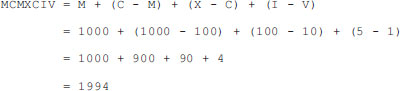
The Roman numeral system is based on an add - subtract rule whereby the elements of a number, read left-to-right, are either added to or subtracted from the previous sum according to its value. Thereby, the decimal number 1994 is represented in Roman numerals as follows:
The uncertainty in the positional value of each digit, the absence of a symbol for zero, and the fact that some numbers require either one or two symbols (I, IV, V, IX, and X) complicate the rules of arithmetic using Roman numerals.
C.2 Origins of the Decimal System
The one element of our civilization that has transcended all cultural and social differences is our decimal system of numbers. While mankind is yet to agree on the most desirable political order, on generally acceptable rules of moral behavior, or on a universal language, the Hindu-Arabic numerals have been adopted by practically all the nations and cultures of the world.
By the ninth century A.D. the Arabs were using a ten-symbol positional system of numbers that included the special symbol for 0. The Latin title of the first book on the subject of “Indian numbers” is Liber Algorismi de Numero Indorum. The author is the Arab mathematician al-Khowarizmi.
Despite of the evident advantages of this number system, its adoption in Europe took place only after considerable debate and controversy. Many scholars of the time still considered Roman numerals to be easier to learn and more convenient for operations on the abacus. The supporters of the Roman numeral system, called abacists, engaged in intellectual combat with the algorists, who were in favor of the Hindu-Arabic numerals as described by al-Khowarizmi. For several centuries abacists and algorists debated about the advantages of their systems, with the Catholic church often siding with the abacists. This controversy explains why the Hindu-Arabic numerals were not accepted into general use in Europe until the beginning of the sixteenth century.
It is sometimes said that the reason for there being ten symbols in the Hindu-Arabic numerals is related to the fact that we have ten fingers. However, if we make a one-to-one correlation between the Hindu-Arabic numerals and our fingers, we find that the last finger must be represented by a combination of two symbols, 10. Also, one Hindu-Arabic symbol, 0, cannot be matched to an individual finger. In fact, the decimal system of numbers, as used in a positional notation that includes a zero digit, is a refined and abstract scheme that should be considered one of the greatest achievements of human intelligence. We will never know for certain if the Hindu-Arabic numerals are related to the fact that we have ten fingers, but its profoundness and usefulness clearly transcend this biological fact.
The most significant feature of the Hindu-Arabic numerals is the presence of a special symbol, 0, which by itself represents no quantity. Nevertheless, the special symbol 0 is combined with the other ones. In this manner the nine other symbols are reused to represent larger quantities. Another characteristic of decimal numbers is that the value of each digit depends on its position in a digit string. This positional characteristic, in conjunction with the use of the special symbol 0 as a placeholder, allow the following representations:

The result is a counting scheme where the value of each symbol is determined by its column position. This positional feature requires the use of the special symbol, 0, which does not correspond to any unit-amount, but is used as a placeholder in multicolumn representations. We must marvel at the intelligence, capability for abstraction, and even the sense of humor of the mind that conceived a counting system that has a symbol that represents nothing. We must also wonder about the evolution of mathematics, science, and technology had this system not been invented. One intriguing question is whether a positional counting system that includes the zero symbol is a natural and predictable step in the evolution of our mathematical thought, or whether its invention was a stroke of genius that could have been missed for the next two thousand years.
C.2.1 Number Systems for Digital-Electronics
The computers built in the United States during the early 1940s operated on decimal numbers. However, in 1946, von Neumann, Burks, and Goldstine published a trend-setting paper titled “Preliminary Discussion of the Logical Design of an Electronic Computing Instrument,” in which they state:
“In a discussion of the arithmetic organs of a computing machine one is naturally led to a consideration of the number system to be adopted. In spite of the long-standing tradition of building digital machines in the decimal system, we must feel strongly in favor of the binary system for our device.”
In their paper, von Neumann, Burks, and Goldstine also consider the possibility of a computing device that uses binary-coded decimal numbers. However, the idea is discarded in favor of a pure binary encoding. The argument is that binary numbers are more compact than binary-coded decimals. Later in this book you will see that binary-coded decimal numbers (called BCD) are used today in some types of computer calculations.
In 1941, Konrad Zuse, a German who had done pioneering work in computing machines, released the first programmable computer designed to solve complex engineering equations. The machine, called the Z3, was controlled by perforated strips of discarded movie film and used the binary number system.
The use of the binary number system in digital calculators and computers was made possible by previous research on number systems and on numerical representations, starting with an article by G.W. Leibnitz published in Paris in 1703. Re searchers concluded that it is possible to count and perform arithmetic operations using any set of symbols as long as the set contains at least two symbols, one of which must be zero.
In digital electronics the binary symbol 1 is equated with the electronic state ON, and the binary symbol 0 with the state OFF. The two symbols of the binary system can also represent conducting and nonconducting states, positive or negative, or any other bi-valued condition. It was the binary system that presented the Hindu-Arabic decimal number system with the first challenge in 800 years. In digital-electronics, two steady states are easier to implement and more reliable than a ten-digit encoding.
C.2.2 Positional Characteristics
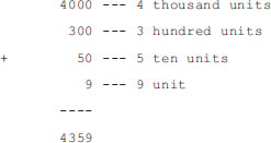
All modern number systems, including decimal, hexadecimal, and binary, are positional and include the digit zero. It is the positional feature that is used to determine the total value of a multi-digit representation. For example, the digits in the decimal number 4359 have the following positional weights:

The total value is obtained by adding the column weights of each unit:
C.2.3 Radix or Base of a Number System
In any positional number system, the weight of each column is determined by the total number of symbols in the set, including zero. This is called the base or radix of the system. The base of the decimal system is 10 and the base of the binary system is 2. The positional value or weight (P) of a digit in a multi-digit number is determined by the formula
where d is the digit, B is the base or radix, and c is the zero-based column number, starting from right to left. Note that the increase in column weight from right to left is purely conventional. You could construct a number system in which the column weights increase in the opposite direction. In fact, in the original Hindu notation, the most significant digit was placed at the right.
In radix-positional terms, a decimal number can be expressed as a sum of digits by the formula
where i is the system’s range and n is its limit.
By the adoption of special representations for different types of numbers, the usefulness of a positional number system can be extended beyond the simple counting function.
The digits of a number system, called the positive integers or natural numbers, are an ordered set of symbols. The notion of an ordered set means that the numerical symbols are assigned a predetermined sequence. A positional system of numbers also requires the special digit zero that, by itself, represents the absence of oneness, or nothing, and thus is not included in the set of natural numbers. However, 0 assumes a cardinal function when it is combined with other digits, for instance, 10 or 30. The whole numbers are the set of natural numbers, including the number zero.
A number system can also encode direction. We generally use the + and − signs to represent opposite numerical directions. The typical illustration for a set of signed numbers is as follows:
![]()
The number zero, which separates the positive and the negative numbers, has no sign of its own; although in some binary encodings we can end up with a negative and a positive zero.
C.3.3 Rational, Irrational, and Imaginary Numbers
A number system also represents parts of a whole. For example, when a carpenter cuts one board into two boards of equal length, we can represent the result with the fraction 1/2; the fraction 1/2 represents one of the two parts that make up the object. Rational numbers are those expressed as a ratio of two integers, for example, 1/2, 2/3, 5/248. Note that this use of the word “rational” is related to the mathematical concept of a ratio, and not to reason.
The denominator of a rational number expresses the number of potential parts. In this sense 2/5 indicates two of five possible parts. There is no reason why the number 1 cannot be used to indicate the number of potential parts, for example 2/1, 128/1. In this case the ratio x/1 indicates x elements of an undivided part. Therefore, it follows that x/1 = x. The implication is that the set of rational numbers includes the integers, because an integer can be expressed as a ratio using a unit denominator.
But not all non-integer numbers can be written as an exact ratio of two integers. The discovery of the first irrational number is usually associated with the investigation of a right triangle by the Greek mathematician Pythagoras (approximately 600 B.C.). The Pythagorean Theorem states that in any right triangle the square of the longest side (hypotenuse) is equal to the sum of the squares of the other two sides.
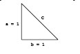
For this triangle, the Pythagorean theorem states that
Therefore, the length of the hypotenuse in a right triangle with unit sides is a number, that when multiplied by itself, gives 2. This number (approximately 1.414213562) cannot be expressed as the exact ratio of two integers. Other irrational numbers are the square roots of 3 and 5, as well as the mathematical constants π and e.
The set of numbers that includes the natural numbers, the whole numbers, and the rational and irrational numbers is called the real numbers. Most common mathematical problems are solved using real numbers. However, during the investigation of squares and roots, we notice that there can be no real number whose square is negative. Mathematicians of the eighteenth century extended the number system to include operations with roots of negative numbers. They did this by defining an imaginary unit as follows:
The imaginary unit makes possible new set of numbers, called complex numbers, that consist of a real part and an imaginary part. One of the uses of complex numbers is in finding the solution of a quadratic equation. Complex numbers are also useful in vector analysis, graphics, and in solving many engineering, scientific, and mathematical problems.
The radix of a number system is the number of symbols in the set, including zero. Thus, the radix of the decimal system is 10, and the radix of the binary system is 2. Digital electronics is based on circuits that can be in one of two stable states. Therefore, a number system based on two symbols is better suited for work in digital electronics, because each state can be represented by a digit.
C.4.1 Decimal versus Binary Numbers
The binary system of numbers uses two symbols, 1 and 0. It is the simplest possible set of symbols with which we can count and perform arithmetic. Most of the difficulties in learning and using the binary system arise from this simplicity. Figure C.1 shows sixteen groups of four electronic cells each in all possible combinations of two states.

Figure C-1 Electronic Cells and Binary Numbers
It is interesting to note that binary numbers match the physical state of each electronic cell. If we think of each cell as a miniature light bulb, then the binary number 1 can be used to represent the state of a charged cell (light ON) and the binary number 0 to represent the state of an uncharged cell (light OFF).
Binary numbers are convenient in digital electronics; however, one of their drawbacks is the number of symbols required to encode a large value. For example, the number 9134 is represented in four decimal digits. However, the binary equivalent 10001110101110 requires fourteen digits. In addition, large binary numbers are difficult to remember.
One possible way of compensating for these limitations of binary numbers is to use individual symbols to represent groups of binary digits. For example, a group of three binary numbers allow eight possible combinations. In this case, we can use the decimal digits 0 to 7 to represent each possible combination of three binary digits. This grouping of three binary digits gives rise to the following table:
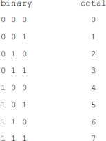
The octal encoding serves as a shorthand representation for groups of three-digit binary numbers.
Hexadecimal numbers (base 16) are used for representing values encoded in four binary digits. Because there are only ten decimal digits, the hexadecimal system borrows the first six letters of the alphabet (A, B, C, D, E, and F). The result is a set of sixteen symbols, as follows:
![]()
Most modern computers are desgined with memory cells, registers, and data paths in multiples of four binary digits. Table C.2 lists some common units of memory storage.
Table C.2
Units of Memory Storage
Unit |
Bits |
Hex Digits |
Hex Range |
Nibble |
4 |
1 |
0 to F |
Byte |
8 |
2 |
0 to FF |
Word |
16 |
4 |
0 to FFFF |
Doubleword |
32 |
8 |
0 to FFFFFFFF |
In most digital-electronic devices memory addressing is organized in multiples of four binary digits. Here again, the hexadecimal number system provides a convenient way to represent addresses. Table C.3 lists some common memory addressing units and their hexadecimal and decimal range.
Table C.3
Units of Memory Addressing
Unit |
Data Path |
Address Range |
|
IN BITS |
DECIMAL |
HEX |
|
1 paragraph |
4 |
0 to 15 |
0-F |
1 page |
8 |
0 to 255 |
0-FF |
1 kilobyte |
16 |
0 to 65,535 |
0-FFFF |
1 megabyte |
20 |
0 to 1,048,575 |
0-FFFFF |
4 gigabytes |
32 |
0 to 4,294,967,295 |
0-FFFFFFFF |
We use decimal numbers in our everyday life because they meaningfully represent common units used in the real world. To state that a certain historical event took place in the year 7C6 hexadecimal would convey little information to the average person. However, in computer systems based on two-state electronic cells, binary representations are more convenient. Also note that hexadecimal and octal numbers are handy shorthand for representing groups of binary digits.
Numerical conversions between positional systems of different radices are based on the number of symbols in the respective sets and on the positional value (weight) of each column. But methods used for manual conversions are not always suitable for machine conversions, as we will see in the forthcoming sections.
To manually convert a binary number to its decimal equivalent we take into account the positional weight of each binary digit, as shown in Figure C-2.
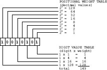
Figure C-2 Binary to ASCII Decimal Conversion Example
The positional weight table in Figure C-2 lists the decimal value of each binary column. These weights are powers of the system’s base (2 in the binary system). In the digit value table, also in Figure C-2, the decimal values of the binary columns holding a 1 digit are added. The sum of the weights of all the 1-digits in the operand is the decimal equivalent of the binary number. In this case, 10010101 binary = 149 decimal.
The method in Figure C-2, although useful in manual conversions, is not an algorithm for computer conversions. Figure C-3 is a flowchart of a low-level binary-to-decimal conversion routine.
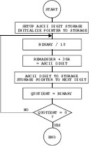
Figure C-3 Flowchart for a Binary to ASCII Decimal Conversion
The algorithm for the processing in Figure C-3 can be written as follows:
1. Set up and initialize a string storage area (sometimes called a buffer) to hold the ASCII decimal digits of the result. Set up the buffer pointer to the rightmost digit position of the result.
2. Obtain the remainder of the value divided by 10.
3. Add 30H to remainder digit to convert to ASCII representation.
4. Store remainder digit in buffer and index the buffer pointer to the preceding digit.
5. Quotient of division by 10 becomes the new binary value.
6. End conversion routine if quotient is equal to 0. Otherwise, continue at Step 2.
Note that the numerical digits are located from 30H to 39H in the ASCII table. This makes is easy to convert a binary digit to ASCII simply by adding 30H. Likewise, an ASCII digit is converted to binary by subtracting 30H.
C.5.2 Binary-to-Hexadecimal Conversion
The method described in Section 2.4.1 for a binary-to-ASCII decimal conversion can be adapted to other radices by representing the positional weight of each binary digit in the number system to which the conversion is to be made. In the case of a binary-to-ASCII hexadecimal conversion the positional weight of each binary digit is a hexadecimal value. Figure C-4 shows the conversion of the binary value 10010101 into hexadecimal using the corresponding positional weights.
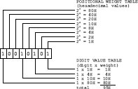
Figure C-4 Binary to ASCII Hexadecimal Conversion Example
The machine conversion binary-to-ASCII hexadecimal is similar to the binary-to-ASCII decimal algorithm described previously. In the case of the conversion into ASCII hexadecimal digits, the buffer need only hold four ASCII characters, because a 16-bit binary cannot exceed the value FFFFH. In the case of binary-to-ASCII hex, the divisor for obtaining the digits is 16 instead of 10.
C.5.3 Decimal-to-Binary Conversion
Longhand conversion of decimal into binary can be performed using the positional weights to find the binary 1 digits and then subtracting this positional weight from the decimal value. The process is shown in Figure C-5.

Figure C-5 Example of Decimal-to-Binary Conversion
In the example of Figure C-5, we start with the decimal value 149. Because the highest power of 2 smaller than 149 is 128, which corresponds to bit 7, we set bit 7 in the result and perform the subtraction:
![]()
At this point the highest positional weight smaller that 21 is 16, which corresponds to bit 4. Therefore we set bit 4 and perform the subtraction:
![]()
The remaining steps in the conversion can be seen in the illustration. The conversion is finished when the result of the subtraction is 0.
Suppose there is a numerical value in the form of a string of ASCII decimal, octal, or hexadecimal digits. In order for a processor to perform simple arithmetic operations on such data, the data must first be converted to binary. The binary value is then loaded into machine registers or memory cells. However, methods suited for manual conversion do not always make a good computer algorithm. Figure C.6 shows two decimal-to-binary conversion algorithms that are suited for machine coding.
Using the first method of Figure C-6, the individual decimal digits are multiplied by their corresponding positional values. The final result is obtained by adding all the partial products. Although this method is frequently used, it has the disadvantage that a different multiplier is used during each iteration (1, 10, 100, 1000). The second method in Figure C-6 starts with the high-order ASCII-decimal digit. The calculations consist of multiplying an accumulated value by 10. Initially, this accumulated value is set to 0. After multiplication by 10, the value of the digit is added to the accumulated value. The following algorithm is based on the second method in Figure C-6
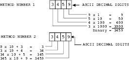
Figure C-6 Machine Conversion of ASCII Decimal to Binary.
1. Set up and initialize to binary zero a storage location for holding the value accumulated during conversion. Set up a pointer to the highest-order ASCII digit in the source string.
2. Test the ASCII digit for a value in the range 0 to 9. End of routine if the ASCII digit is not in this range.
3. Subtract 30H from ASCII decimal digit.
4. Multiply accumulated value by 10.
5. Add digit to accumulated value.
6. Increment the pointer to the next digit and continue at Step 2.
Figure C-7 is a flowchart of the conversion algorithm
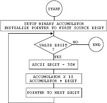
Figure C-7 Flowchart for ASCII to Machine Register Conversion.