4.3. Location Estimation

In this section, we show that in the context of computer vision tasks, often only nonparametric approaches can provide a robust solution for the location estimation problem. We employ a class of nonparametric techniques in which the data points are regarded as samples from an unknown probability density. The location estimates are then defined as the modes of this density. Explicit computation of the density is avoided by using the mean shift procedure.

4.3.1. Why nonparametric methods?

The most general model of the location problem is that of multiple structures,

Equation 4.63

with no information being available about the nature of the inlier noise δy_i the n — n₁ outliers, or the number of structures present in the data K. The model (4.63) is also used in duster analysis, the equivalent pattern recognition problem. Clustering under its most general form is an unsupervised learning method of unknown categories from incomplete prior information [52, p. 242]. The books [52], [21, Chap. 10], [44, Sec. 14.3] provide a complete coverage of the related pattern recognition literature.

Many of the pattern recognition methods are not adequate for data analysis in computer vision. To illustrate their limitations, we compare the two data sets shown in Figure 4.9. The data in Figure 4.9a obeys what is assumed in traditional clustering methods when the proximity to a cluster center is measured as a function of Euclidean or Mahalanobis distances. In this case, the shape of the clusters is restricted to elliptical, and the inliers are assumed to be normally distributed around the true cluster centers. A different metric will impose a different shape on the clusters. The number of the structures (clusters) K is a parameter to be supplied by the user and has a large influence on the quality of the results. While the value of K can be also derived from the data by optimizing a cluster validity index, this approach is not robust, since it is based on (possibly erroneous) data partitions.

Expectation maximization (EM) is a frequently used technique today in computer vision to model the data. See [44, Sec. 8.5.2] for a short description. The EM algorithm also relies on strong prior assumptions. A likelihood function, defined from a mixture of predefined (most often normal) probability densities, is maximized. The obtained partition of the data thus employs "tiles" of given shape. The number of required mixture components is often difficult to determine, and the association of these components with true cluster centers may not be obvious.

Examine now the data in Figure 4.9b in which the pixels of a color image were mapped into the 3D L*u*v* color space. The significant clusters correspond to similarly colored pixels in the image. The clusters have a large variety of shapes and their number is not obvious. Any technique that imposes a preset shape on the clusters will have difficulties accurately separating K significant structures from the background clutter while simultaneously also having to determine the value of K.

Following our goal-oriented approach toward robustness (Section 4.2.3), a location estimator should be declared robust only if it returns a satisfactory result. From the above discussion, we can conclude that robustly solving location problems in computer vision often requires techniques that use the least possible amount of prior assumptions about the data. Such techniques belong to the family of nonparametric methods.

In nonparametric methods, the n data points are regarded as outcomes from an (unknown) probability distribution f(y). Each data point is assumed to have an equal probability

Equation 4.64

When several points have the same value, the probability is n^-1 times the multiplicity. The ensemble of points defines the empirical distribution f(y|y₁ ...y_n) of the data. The empirical distribution is the nonparametric maximum likelihood estimate of the distribution from which the data was drawn [22, p. 310]. It is also the "least committed" description of the data.

Every clustering technique exploits the fact that the clusters are the denser regions in the space. However, this observation can be pushed further in the class of nonparametric methods considered here, for which a region of higher density implies more probable soutcomes of the random variable y. Therefore, in each dense region, the location estimate (cluster center) should be associated with the most probable value of y, that is, with the local mode of the empirical distribution

Equation 4.65

Note that by detecting all the significant modes of the empirical distribution, the number of clusters K is automatically determined. The mode-based clustering techniques make extensive use of density estimation during data analysis.

4.3.2. Kernel density estimation

The modes of a random variable y are the local maxima of its probability density function f(y). However, only the empirical distribution, the data points y_i, i = 1,..., n, are available. To accurately determine the locations of the modes, first a continuous estimate of the underlying density has to be defined. Later we will see that this step can be eliminated by directly estimating the gradient of the density (Section 4.3.3).

To estimate the probability density in y, a small neighborhood is defined around y. The neighborhood usually has a simple shape: cube, sphere, or ellipsoid. Let its volume be V_y, and m_y be the number of data points inside. Then the density estimate is [21, Sec. 4.21]

Equation 4.66

which can be employed in two different ways.

- In the nearest neighbors approach, the neigborhoods (the volumes V_y) are scaled to keep the number of points m_y constant. A mode corresponds to a location in which the neighborhood has the smallest volume.

- In the kernel density approach, the neigborhoods have the same volume V_y and the number of points m_y inside are counted. A mode corresponds to a location in which the neighborhood contains the largest number of points.

The minimum volume ellipsoid (MVE) robust location estimator proposed in statistics [89, p. 258] is a technique related to the nearest neighbors approach. The ellipsoids are defined by elemental subsets obtained through random sampling, and the numerical optimization procedure discussed in Section 4.2.7 is employed. The location estimate is the center of the smallest ellipsoid, which contains a given percentage of the data points. In a robust clustering method proposed in computer vision, the MVE estimator was used to sequentially remove the clusters from the data, starting from the largest [53]. However, by imposing an elliptical shape for the clusters, severe artifacts were introduced and the method was never successful in real vision applications.

For our goal of finding the local maxima of , the kernel density methods are more suitable. Kernel density estimation is a widely used technique in statistics and pattern recognition, where it is also called the Parzen window method. See [92, 112] for a description in statistics, and [21, Sec. 4.3] [44, Sec. 6.6] for a description in pattern recognition.

We start with the simplest case of 1D data. Let y_i, i = 1,...,n, be scalar measurements drawn from an arbitrary probability distribution f(y). The kernel density estimate of this distribution is obtained based on a kernel function K(u) and a bandwidth h as the average

Equation 4.67

Only the class of symmetric kernel functions with bounded support will be considered. They satisfy the following properties:

Equation 4.68

Other conditions on the kernel function or on the density to be estimated [112, p. 18], are of less significance in practice. The even symmetry of the kernel function allows us to define its profile k(u):

Equation 4.69

where c_k is a normalization constant determined by (4.68). The shape of the kernel implies that the profile is a monotonically decreasing function.

The kernel density estimate is a continuous function derived from the discrete data, the empirical distribution. An example is shown in Figure 4.10. When instead of the histogram of the n points (Figure 4.10a) the data is represented as an ordered list (Figure 4.10b, bottom), we are in fact using the empirical distribution. By placing a kernel in each point (Figure 4.10b), the data is convolved with the symmetric kernel function. The density estimate in a given location is the average of the contributions from each kernel (Figure 4.10c). Since the employed kernel has a finite support, not all the points contribute to a density estimate. The bandwidth h scales the size of the kernels, i.e., the number of points whose contribution is averaged when computing the estimate. The bandwidth thus controls the amount of smoothing present in .

For multivariate measurements y_i ∊ R^p, in the most general case, the bandwidth h is replaced by a symmetric, positive definite bandwidth matrix H. The estimate of the probability distribution at location y is still computed as the average

Equation 4.70

where the bandwidth matrix H scales the kernel support to be radial symmetric, that is, to have the desired elliptical shape and size

Equation 4.71

Since only circular symmetric prototype kernels K(u) are considered, we have, using the profile k(u),

Equation 4.72

From (4.70), taking into account (4.72) and (4.71) results in

Equation 4.73

where the expression d[y, y_i, H]² denotes the squared Mahalanobis distance from y to y_i. The case H = h²I_p is the most often used. The kernels then have a circular support whose radius is controlled by the bandwidth h, and (4.70) becomes

Equation 4.74

where the dependence of the density estimate on the kernel was made explicit.

The quality of a density estimate is assessed in statistics using the asymptotic mean integrated error (AMISE), that is, the integrated mean square error

Equation 4.75

between the true density and its estimate for n → ∞, while h → 0 at a slower rate. The expectation is taken over all data sets of size n. Since the bandwidth h of a circular symmetric kernel has a strong influence on the quality of , the bandwidth minimizing an approximation of the AMISE error is of interest. Unfortunately, this bandwidth depends on f (y), the unknown density [112, Sec. 4.3].

For the univariate case, several practical rules are available [112, Sec. 3.2]. For example, the information about f(y] is substituted with , a robust scale estimate derived from the data

Equation 4.76

where

Equation 4.77

The scale estimate is discussed in Section 4.4.3.

For a given bandwidth, the AMISE measure is minimized by the Epanechnikov kernel [112, p. 104] having the profile

Equation 4.78

which yields the kernel

Equation 4.79

where c_p is the volume of the p-dimensional unit sphere. Other kernels can also be defined. The truncated normal has the profile

Equation 4.80

where a is chosen such that e−^a is already negligibly small. Neither of the two profiles defined above has continuous derivatives at the boundary u = 1. This condition is satisfied (for the first two derivatives) by the biweight kernel having the profile

Equation 4.81

Its name here is taken from robust statistics; in the kernel density estimation literature, it is called the triweight kernel [112, p. 31].

The bandwidth matrix H is the critical parameter of a kernel density estimator. For example, if the region of summation (bandwidth) is too large, significant features of the distribution, like multimodality, can be missed by oversmoothing. Furthermore, locally the data can have very different densities, and using a single bandwidth matrix often is not enough to obtain a satisfactory estimate.

There are two ways to adapt the bandwidth to the local structure. In each case, the adaptive behavior is achieved by first performing a pilot density estimation. The bandwidth matrix can be associated with the location y in which the distribution is to be estimated, or else each measurement y_i can be taken into account in (4.70) with its own bandwidth matrix:

Equation 4.82

It can be shown that (4.82), called the sample point density estimator, has superior statistical properties [39].

The local maxima of the density f(y) are by definition the roots of the equation

Equation 4.83

that is, the zeros of the density gradient. Note that the converse is not true, since any stationary point of f(y) satisfies (4.83). The true density, however, is not available, and in practice, the estimate of the gradient has to be used.

In the next section, we describe the mean shift technique, which avoids explicit computation of the density estimate when solving (4.83). The mean shift procedure also associates each data point to the nearest density maximum and thus performs a nonparametric clustering in which the shape of the clusters is not set a priori.

4.3.3. Adaptive mean shift

The mean shift method was described in several publications [16, 18, 17]. Here we consider its most general form in which each measurement y_i is associated with a known bandwidth matrix H_i, i = 1,...,n. Taking the gradient of the sample point density estimator (4.82), we obtain, after recalling (4.73) and exploiting the linearity of the expression,

Equation 4.84

The function g(x) = -k′(x) satisfies the properties of a profile, and thus we can define the kernel G(u) = c_g,pg(u^T u). For example, for the Epanechnikov kernel, the corresponding new profile is

Equation 4.85

and thus G_E(u) is the uniform kernel. For convenience, we introduce the notation

Equation 4.86

From the definition of g(u) and (4.69),

Equation 4.87

Then (4.84) can be written as

Equation 4.88

and the roots of the equation (4.83) are the solutions of

Equation 4.89

which can be solved only iteratively

Equation 4.90

The meaning of an iteration becomes apparent if we consider the particular case yielding

Equation 4.91

which becomes, when all hi = h,

Equation 4.92

From (4.87) we see that at every step only a local weighted mean is computed. The robustness of the mode detection method is the direct consequence of this property. In the next iteration, the computation is repeated centered on the previously computed mean. The difference between the current and previous locations, the vector

Equation 4.93

is called the mean shift vector, where the fact that the weighted averages are computed with the kernel G was made explicit. Adapting (4.88) to the two particular cases above, it can be shown that

Equation 4.94

where c is a positive constant. Thus, the mean shift vector is aligned with the gradient estimate of the density, and the window of computations is always moved toward regions of higher density. See [17] for the details. A relation similar to (4.94) still holds in the general case, but now the mean shift and gradient vectors are connected by a linear transformation.

In the mean shift procedure, the user controls the resolution of the data analysis by providing the bandwidth information. Since most often circular symmetric kernels are used, only the bandwidth parameters hi are needed.

Mean Shift Procedure

1.	Choose a data point yi as the initial y[0].
2.	Compute y[l+1], l = 0,1,... the weighted mean of the points at less than unit Mahalanobis distance from y[l]. Each point is considered with its own metric.
3.	Determine if is less than the tolerance. If yes, stop.
4.	Replace y[l] with y[l+1]; that is, move the processing toward a region with higher point density. Return to Step 2.

The most important properties of the mean shift procedure are illustrated graphically in Figure 4.11. In Figure 4.11a, the setup of the weighted mean computation in the general case is shown. The kernel associated with a data point is nonzero only within the elliptical region centered on that point. Thus, only those points contribute to the weighted mean in y whose kernel support contains y.

The evolution of the iterative procedure is shown in Figure 4.11b for the simplest case of identical circular kernels (4.92). When the locations of the points in a window are averaged, the result is biased toward the region of higher point density in that window. By moving the window into the new position, we move uphill on the density surface. The mean shift procedure is a gradient ascent technique. The processing climbs toward the highest point on the side of the density surface on which the initial position y^[0] was placed. At convergence (which can be proven), the local maximum of the density, the sought mode, is detected.

The two initializations in Figure 4.11b are on different components of this mixture of two Gaussians. Therefore, while the two mean shift procedures start from nearby locations, they converge to different modes, both of which are accurate location estimates.

A nonparametric classification of the data into clusters can be obtained by starting a mean shift procedure from every data point. A set of points converging to nearby locations defines the basin of attraction of a mode. Since the points are processed independently, the shape of the basin of attraction is not restricted in any way. The basins of attraction of the two modes of a Gaussian mixture (Figure 4.11c) were obtained without using the nature of the distributions.

The 2D data in Figure 4.12a illustrates the power of the mean shift-based clustering. The three clusters have arbitrary shapes, and the background is heavily cluttered with outliers. Traditional clustering methods would have difficulty yielding satisfactory results. The three significant modes in the data are clearly revealed in a kernel density estimate (Figure 4.12b). The mean shift procedure detects all three modes, and the associated basins of attraction provide a good delineation of the individual clusters (Figure 4.12c). In practice, using only a subset of the data points suffices for an accurate delineation. See [16] for details of the mean shift-based clustering.

The original mean shift procedure was proposed in 1975 by Fukunaga and Hostetler [32]. See also [31, p. 535]. It came again into attention with the paper [10]. In spite of its excellent qualities, mean shift is less known in the statistical literature. The book [92, Sec. 6.2.2] discusses [32], and a similar technique is proposed in [11] for bias reduction in density estimation.

The simplest, fixed-bandwidth mean shift procedure in which all H_i = h²I_p is the one most frequently used in computer vision applications. The adaptive mean shift procedure discussed in this section, however, is not difficult to implement with circular symmetric kernels: . The bandwidth value hi associated with the data point y_i can be defined as the distance to the k-th neighbor; that is, for the pilot density estimation, the nearest neighbors approach is used. An implementation for high dimensional spaces is described in [35]. Other, more sophisticated methods for local bandwidth selection are described in [15, 18]. Given the complexity of the visual data, such methods, which are based on assumptions about the local structure, may not provide any significant gain in performance.

4.3.4. Applications

We now sketch two applications of the fixed-bandwidth mean shift procedure, that is, circular kernels with H_i = h²I_p.

- discontinuity preserving filtering and segmentation of color images;

- tracking of nonrigid objects in a color image sequence.

These applications are the subject of [17] and [19] respectively, which should be consulted for details.

An image can be regarded as a vector field defined on the 2D lattice. The dimension of the field is one in the gray-level case and three for color images. The image coordinates belong to the spatial domain, while the gray level or color information is in the range domain. To be able to use in the mean shift procedure circular symmetric kernels, the validity of an Euclidean metric must be verified for both domains. This is most often true in the spatial domain and for gray-level images in the range domain. For color images, mapping the RGB input into the L*u*v* (or L*a*b*) color space provides the closest possible Euclidean approximation for the perception of color differences by human observers.

The goal in image filtering and segmentation is to generate an accurate, piecewise-constant representation of the input. The constant parts should correspond in the input image to contiguous regions with similarly colored pixels, while the discontinuities should correspond to significant changes in color. This is achieved by considering the spatial and range domains jointly. In the joint domain, the basin of attraction of a mode corresponds to a contiguous, homogeneous region in the input image, and the valley between two modes most often represents a significant color discontinuity in the input. The joint mean shift procedure uses a product kernel

Equation 4.95

where y^s and y^r are the spatial and the range parts of the feature vector, k(u) is the profile of the kernel used in both domains (though they can also differ), h_s and h_r are the employed bandwidths parameters, and c is the normalization constant. The dimension of the range domain q is one for the gray level and three for the color images. The user sets the value of the two bandwidth parameters according to the desired resolution of the image analysis.

In discontinuity preserving filtering, every pixel is allocated to the nearest mode in the joint domain. All the pixels in the basin of attraction of the mode get the range value of that mode. From the spatial arrangement of the basins of attraction, the region adjacency graph (RAG) of the input image is then derived. A transitive closure algorithm is performed on the RAG, and the basins of attraction of adjacent modes with similar range values are fused. The result is the segmented image.

The gray-level image example in Figure 4.13 illustrates the role of the mean shift procedure. The small region of interest (ROI) in Figure 4.13a is shown in a wireframe representation in Figure 4.13b. The 3D G kernel used in the mean shift procedure (4.92) is in the top left corner. The kernel is the product of two uniform kernels: a circular, symmetric 2D kernel in the spatial domain and a ID kernel for the gray values.

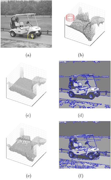
At every step of the mean shift procedure, the average of the 3D data points is computed and the kernel is moved to the next location. When the kernel is defined at a pixel on the high plateau on the right in Figure 4.13b, adjacent pixels (neighbors in the spatial domain) have very different gray-level values and will not contribute to the average. This is how the mean shift procedure achieves the discontinuity preserving filtering. Note that the probability density function whose local mode is sought cannot be visualized, since it would require a 4D space, the fourth dimension being that of the density.

The result of the segmentation for the ROI is shown in Figure 4.13c and for the entire image in Figure 4.13d. A more accurate segmentation is obtained if edge information is incorporated into the mean shift procedure (Figures 4.13e and 4.13f). The technique is described in [13].

A color image example is shown in Figure 4.14. The input has large homogeneous regions, and after filtering (Figures 4.14b and 4.14c), many of the delineated regions already correspond to semantically meaningful parts of the image. However, this is more the exception than the rule in filtering. A more realistic filtering process can be observed around the windows, where many small regions (basins of attraction containing only a few pixels) are present. These regions are either fused or attached to a larger neighbor during the transitive closure process on the RAG, and the segmented image (Figures 4.14d and 4.14e) is less cluttered. The quality of any segmentation, however, can be assessed only through the performance of subsequent processing modules for which it serves as input.

The discontinuity preserving filtering and the image segmentation algorithm were integrated with a novel edge detection technique [73] in the Edge Detection and Image SegmentatiON (EDISON) system [13]. The C++ source code of EDISON is available on the web at

www.caip.rutgers.edu/riul/.

The second application of the mean shift procedure is tracking of a dynamically changing neighborhood in a sequence of color images. This is a critical module in many object recognition and surveillance tasks. The problem is solved by analyzing the image sequence as pairs of two consecutive frames. See [19] for a complete discussion.

The neighborhood to be tracked (i.e., the target model in the first image) contains n_a pixels. We are interested only in the amount of relative translation of the target between the two frames. Therefore, without loss of generality, the target model can be considered centered on y_a = 0. In the next frame, the target candidate is centered on y_b and contains n_b pixels.

In both color images, kernel density estimates are computed in the joint 5D domain. In the spatial domain, the estimates are defined in the center of the neighborhoods, while in the color domain, the density is sampled at m locations c. Let c = 1,..., m be a scalar hashing index of these 3D sample points. A kernel with profile k(u) and bandwidths h_a and h_b is used in the spatial domain. The sampling in the color domain is performed with the Kronecker delta function δ(u) as kernel.

The result of the two kernel density estimations are the two discrete color densities associated with the target in the two images. For c = 1,...,m

Equation 4.96

Equation 4.97

where c(y) is the color vector of the pixel at y. The normalization constants A, B are determined such that

Equation 4.98

The normalization assures that the template matching score between these two discrete signals is

Equation 4.99

and it can be shown that

Equation 4.100

is a metric distance between and

To find the location of the target in the second image, the distance (4.100) has to be minimized over y_b, or equivalently (4.99) has to be maximized. That is, the local maximum of ρ(y_b) has to be found by performing a search in the second image. This search is implemented using the mean shift procedure.

The local maximum is a root of the template matching score gradient

Equation 4.101

Taking into account (4.97) yields

Equation 4.102

As in Section 4.3.3, we can introduce the profile g(u) = —k′(u) and define the weights

Equation 4.103

and obtain the iterative solution of (4.101) from

Equation 4.104

which is a mean shift procedure, the only difference being that at each step the weights (4.103) are also computed.

In Figure 4.15, four frames of an image sequence are shown. The target model, defined in the first frame (Figure 4.15a), is successfully tracked throughout the sequence. As can be seen, the localization is satisfactory in spite of the target candidates' color distribution being significantly different from that of the model. While the model can be updated as we move along the sequence, the main reason for the good performance is the small amount of translation of the target region between two consecutive frames. The search in the second image always starts from the location of the target model center in the first image. The mean shift procedure then finds the nearest mode of the template matching score, and with high probability this is the target candidate location we are looking for. See [19] for more examples and extensions of the tracking algorithm, and [14] for a version with automatic bandwidth selection.

The robust solution of the location estimation problem presented in this section put the emphasis on employing the least possible amount of a priori assumptions about the data and belongs to the class of nonparametric techniques. Nonparametric techniques require a larger number of data points supporting the estimation process than their parametric counterparts. In parametric methods, the data is more constrained, and as long as the model is obeyed, the parametric methods are better in extrapolating over regions where data is not available. However, if the model is not correct, a parametric method will still impose it at the price of severe estimation errors. This important tradeoff must be kept in mind when feature space analysis is used in a complex computer vision task.