
5.4. Tensor Voting in 3D
We proceed to the generalization of the framework in 3D. The remainder of this section shows that no significant modifications need to be made, apart from taking into account that more types of perceptual structure exist in 3D than in 2D. In fact, the 2D framework is a subset of the 3D framework, which in turn is a subset of the general ND framework. The second-order tensors and the polarity vectors become 3D, while the voting fields are derived from the same fundamental 2D second-order stick voting field.
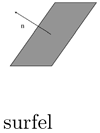
In 3D, the types of perceptual structure that have to be represented are regions (which are now volumes), surfaces, curves, and junctions. Their terminations are the bounding surfaces of volumes, the bounding curves of surfaces, and the endpoints of curves. The inputs can be either unoriented or oriented, in which case there are two types: elementary surfaces (surfels) or elementary curves (curves).
5.4.1. Representation in 3D
The representation of a token consists of a symmetric, second-order tensor that encodes saliency and a vector that encodes polarity.
Second-order representation
A 3D, second-order, symmetric, nonnegative definite tensor is equivalent to a 3 x 3 matrix and a 3D ellipsoid. The eigenvectors of the tensor are the axes of the ellipsoid. It can be decomposed as in the following equation:
Equation 5.9
![]()
where λi are the eigenvalues in decreasing order and êi are the corresponding eigenvectors (see also Figure 5.20). Note that the eigenvalues are non-negative, since the tensor is nonnegative definite, and the eigenvectors are orthogonal. The first term in (5.9) corresponds to a degenerate, elongated ellipsoid, the 3D stick tensor, that indicates an elementary surface token with ê1 as its surface normal. The second term corresponds to a degenerate disk-shaped ellipsoid, termed hereafter the plate tensor, that indicates a curve or a surface intersection with ê3 as its tangent, or, equivalently, with ê1 and ê2 spanning the plane normal to the curve. Finally, the third term corresponds to a sphere, the 3D ball tensor, that corresponds to a structure that has no preference of orientation. Table 5.5 shows how oriented and unoriented inputs are encoded and the equivalent ellipsoids and quadratic forms.
Figure 5.20. A second-order generic tensor and its decomposition in 3D.

| Input | Tensor | Eigenvalues | Quadratic form |
|---|---|---|---|
 | λ1 = 1, λ2 = 1, λ3 = 0 | 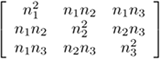 | |
 | λ1 = λ2 = 1, λ3 = 0 | P (see below) | |
 |  | λ1 = λ2 = λ3 = 1 |  |

The representation using normals instead of tangents can be justified more easily in 3D, where surfaces are arguably the most frequent type of structure. In 2D, normal or tangent representations are equivalent. A surface patch in 3D is represented by a stick tensor parallel to the patch's normal. A curve, which can also be viewed as a surface intersection, is represented by a plate tensor that is normal to the curve. All orientations orthogonal to the curve belong in the 2D subspace defined by the plate tensor. Any two of these orientations that are orthogonal to each other can be used to initialize the plate tensor (see also Table 5.5). Adopting this representation allows a structure with N — 1 degrees of freedom in ND (a curve in 2D, a surface in 3D) to be represented by a single vector, while a tangent representation would require the definition of N—1 vectors that form a basis for an (N—1)-D subspace. Assuming that this is the most frequent structure in the ND space, our choice of representation makes the stick voting field, which corresponds to the elementary (N — 1)-D variety, the basis from which all other voting fields are derived.
First-order representation
The first-order part of the representation is, again, a polarity vector whose size indicates the likelihood of the token being a boundary of a perceptual structure and which points toward the half-space where the majority of the token's neighbors are.
5.4.2. Voting in 3D
Identically to the 2D case, voting begins with a set of oriented and unoriented tokens. Again, both second- and first-order votes are cast according to the second-order tensor of the voter.
Second-order voting
In this section, we begin by showing how a voter with a purely stick tensor generates and casts votes, and then we derive the voting fields for the plate and ball cases. We chose to maintain voting as a function of only the position of the receiver relative to the voter and of the voter's preference of orientation. Therefore, we again address the problem of finding the smoothest path between the voter and receiver by fitting arcs of the osculating circle, as described in Section 5.3.1.
Note that the voter, the receiver, and the stick tensor at the voter define a plane. The voting procedure is restricted in this plane, thus making it identical to the 2D case. The second-order vote, which is the surface normal at the receiver under the assumption that the voter and receiver belong to the same smooth surface, is also a purely stick tensor in the plane (see also Figure 5.5). The magnitude of the vote is defined by the same saliency decay,function, duplicated here for completeness.
Equation 5.10
![]()
where s is the are length OP, k is the curvature, c is a constant that controls the decay with high curvature, and σ is the scale of voting. Sparse, token-to-token voting is performed to estimate the preferred orientation of tokens, followed by dense voting during which saliency is computed at every grid position.
First-order voting
Following the above line of analysis, the first-order vote is also on the plane defined by the voter, the receiver, and the stick tensor. As shown in Figure 5.9, the first-order vote cast by a unitary stick tensor at the origin is tangent to the osculating circle. Its magnitude is equal to that of the second-order vote.
Voting Fields
Voting by any 3D tensor takes place by decomposing the tensor into its three components: the stick, the plate, and the ball. Second-order voting fields are used to compute the second-order votes and first-order voting fields for the first-order ones. Votes are retrieved from the appropriate voting field by look-up operations and are multiplied by the saliency of each component. Stick votes are weighted by λ1 - λ2, plate votes by λ2 - λ3, and ball votes by λ3.
The 3D first- and second-order fields can be derived from the corresponding 2D fields by rotation about the voting stick, which is their axis of symmetry. The visualization of the 2D second order stick field in Figure 5.11a is also a cut of the 3D field that contains the stick tensor at the origin.
To show the derivation of the ball voting fields Bi(P) from the stick voting fields, we can visualize the vote at P from a unitary ball tensor at the origin O as the integration of the votes of stick tensors that span the space of all possible orientations. In 2D, this is equivalent to a rotating stick tensor that spans the unit circle at O, while in 3D the stick tensor spans the unit sphere. The 3D ball field can be derived from the stick field S(P), as follows. The first-order ball field is derived from the first-order stick field, and the second-order ball field from the second-order stick field.
Equation 5.11
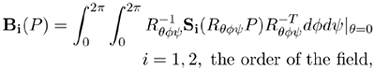
where Rθφψ is the rotation matrix to align S with ê1, the eigenvector corresponding to the maximum eigenvalue (the stick component), of the rotating tensor at P, and θ, φ, ψ are rotation angles about the x-, y-, and z- axes respectively.
In the second-order case, the integration is approximated by tensor addition, ![]() , while in the first-order case by vector addition,
, while in the first-order case by vector addition, ![]() . Note that normalization has to be performed in order to make the energy emitted by a unitary ball equal to that of a unitary stick. Both fields are radially symmetric, as expected, since the voter has no preferred orientation.
. Note that normalization has to be performed in order to make the energy emitted by a unitary ball equal to that of a unitary stick. Both fields are radially symmetric, as expected, since the voter has no preferred orientation.
To complete the description of the voting fields for the 3D case, we need to describe the plate voting fields Pi(P). Since the plate tensor encodes uncertainty of orientation around one axis, it can be derived by integrating the votes of a rotating stick tensor that spans the unit circle: in other words, the plate tensor. The formal derivation is analogous to that of the ball voting fields and can be written as follows:
Equation 5.12

where θ, φ, ψ , and Rθφψ have the same meaning as in the previous equation.
5.4.3. Vote analysis
After voting from token to token has been completed, we can determine which tokens belong to perceptual structures, as well as the type and preferred orientation of these structures. The eigensystem of each tensor is computed, and the tensor is decomposed according to (5.9). Tokens can be classified according to the accumulated first- and second-order information according to Table 5.6.
| 3D feature | Saliency | Second- order tensor orientation | Polarity | Polarity vector |
|---|---|---|---|---|
| surface interior | high λ1 - λ2 | normal: ê1 | low | - |
| surface end-curve | high λ1- λ2 | normal: ê1 | high | orthogonal to ê1 and end-curve |
| curve interior | high λ2 - λ3 | tangent: ê3 | low | - |
| curve endpoint | high λ2 - λ3 | tangent: ê3 | high | parallel to ê3 |
| region interior | high λ3 | - | low | - |
| region boundary | high λ3 | - | high | normal to bounding surface |
| junction | locally max λ3 | - | low | - |
| outlier | low | - | low | - |
Dense structure extraction
Now that the most likely type of feature at each token has been estimated, we want to compute the dense structures (curves, surfaces, and volumes in 3D) that can be inferred from the tokens. Continuous structures are again extracted through the computation of saliency maps. Three saliency maps need to be built: one that contains ê — 2 at every location, one for λ2 — λ3, and one for λ3. This can be achieved by casting votes to all locations, whether they contain a token or not (dense voting).
Surfaces and curves are extracted using a modified marching algorithm [62] (based on the marching cubes algorithm [37]). They correspond to zero crossings of the first derivative of the corresponding saliency. Junctions are isolated and can be detected as distinct local maxima of λ3. Volume inliers are characterized by high λ3 values. Their bounding surfaces also have high λ3 values and high polarity, with polarity vectors being normal to the surface and pointing toward the interior of the region. Volumes are extracted as regions of high λ3, terminated at their boundaries, which have high λ3 and high polarity. Junctions are isolated, distinct maxima of λ3.
In order to reduce the computational cost, the accumulation of votes at locations with no prior information and structure extraction are integrated and performed as a marching process. Beginning from seeds, locations with highest saliency, we perform a dense vote only toward the directions dictated by the orientation of the features. Surfaces are extracted with subvoxel accuracy, as the zero-crossings of the first derivative of surface saliency (Figure 5.21). As in the 2D case, discrete saliency values are computed at grid points, and the continuous function is approximated via interpolation. Locations with high surface saliency are selected as seeds for surface extraction, while locations with high curve saliency are selected as seeds for curve extraction. The marching direction in the former case is perpendicular to the surface normal, while in the latter case, the marching direction is along the curve's tangent (Figure 5.22).
Figure 5.21. Dense surface extraction in 3D. (a) Elementary surface patch with normal  . (b) 3D surface saliency along normal direction. (c) First derivative of surface saliency along normal direction.
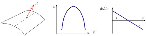
Figure 5.22. Dense curve extraction in 3D. (a) 3D curve with tangent  and the normal plane. (b) Curve saliency isocontours on the normal plane. (c) First derivatives of surface saliency on the normal plane.

5.4.4. Results in 3D
In this section, we present results on synthetic 3D data sets corrupted by random noise. The first example is on a data set that contains a surface in the from of a spiral inside a cloud of noisy points (Figure 5.23). Both the surface and the noise are encoded as unoriented points. The spiral consists of 19,000 points, while the outliers are 30,000. Figure 5.23b shows the surface boundaries detected after voting. As the spiral is tightened to resemble a cylinder (Figure 5.23c), the surfaces merge and the inferred boundaries are those of a cylinder (Figure 5.23d).
Figure 5.23. Surface boundary detection from noisy data.

The example in Figure 5.24 illustrates the detection of regions and curves. The input consists of a "peanut" and a plane, encoded as unoriented points contaminated by random uniformly distributed noise (Figure 5.24a). The "peanut" is empty inside, except for the presence of noise, which has an equal probability of being anywhere in space. Figure 5.24b shows the detected surface inliers after tokens with low saliency have been removed. Figure 5.24c shows the curve inliers, that is the tokens that lie at the intersection of the two surfaces. Finally, Figure 5.24d shows the extracted dense surfaces.
Figure 5.24. Surface and surface intersection extraction from noisy data.
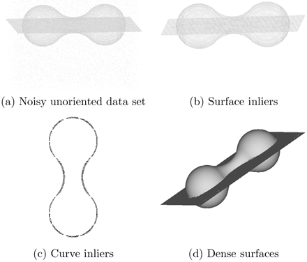
Figure 5.25a shows two solid generalized cylinders with different parabolic sweep functions. The cylinders are generated by a uniform random distribution of unoriented points in their interior, while the noise is also uniformly distributed but with a lower density. After sparse voting, volume inliers are detected due to their high ball saliency and low polarity, while region boundaries are detected due to their high ball saliency and polarity. The polarity vectors are normal to the bounding surface of the cylinders. Using the detected boundaries as inputs, we perform a dense vote and extract the bounding surface in continuous form in Figure 5.25b.
Figure 5.25. Region inlier and boundary detection in 3D.
