9.4. Face Recognition

To date, the appearance-based learning framework has been most influential in the face recognition research. Under this framework, the face recognition problem can be stated as follows: Given a training set, , containing C classes with each class consisting of a number of localized face images z_ij, a total of face images are available in the set. For computational convenience, each image is represented as a column vector of length J(= I_w × I_h) by lexicographic ordering of the pixel elements, that is, z_ij ∊ ^J, where (I_w × I_h) is the image size, and ^J denotes the J-dimensional real space. Taking as input such a set Z, the objectives of appearance-based learning are (1) to find based on optimization of certain separability criteria a low-dimensional feature representation y_ij = ϕ(z_ij), y_ij ∊ ^M, and M ≪ J, with enhanced discriminatory power; (2) to design based on the chosen representation a classifier, , such that h will correctly classify unseen examples ϕ(z, y), where is the class label of z.

9.4.1. Preprocessing

It has been shown that irrelevant facial portions such as hair, neck, shoulder, and background often provide misleading information to the face recognition systems [20]. A normalization procedure is recommended in [95], using geometric locations of facial features found in face detection and alignment. The normalization sequence consists of four steps: (1) the raw images are translated, rotated, and scaled so that the centers of the eyes are placed on specific pixels, (2) a standard mask, as shown in Figure 9.20 (middle) is applied to remove the nonface portions, (3) histogram equalization is performed in the nonmasked facial pixels, and (4) face data are further normalized to have zero mean and unit standard deviation. Figure 9.20 (right) depicts some samples obtained after the preprocessing sequence was applied.

9.4.2. Feature extraction

The goal of feature extraction is to generate a low-dimensional feature representation intrinsic to face objects with good discriminatory power for pattern classification.

PCA subspace

In the statistical pattern recognition literature, PCA [55] is one of the most widely used tools for data reduction and feature extraction. The well-known face recognition method, eigenfaces [122] built on the PCA technique, has proven to be very successful. In the eigenfaces method [122], the PCA is applied to the training set Z to find the N eigenvectors (with nonzero eigenvalues) of the set's covariance matrix,

Equation 9.45

where is the average of the ensemble. The eigenfaces are the first M(≤ N) eigenvectors (denoted as Ψ_ef) corresponding to the largest eigenvalues, and they form a low-dimensional subspace, called face space where most energies of the face manifold are supposed to lie. Figure 9.21 (row 1) shows the first six eigenfaces, which appear, some researchers say, as ghostly faces. Transforming to the M-dimensional face space is a simple linear mapping: , where the basis vectors Ψ_ef are orthonormal. The subsequent classification of face patterns can be performed in the face space using any classifier.

Dual PCA subspaces

The eigenfaces method is built on a single PCA, which suffers from a major drawback; that is, it cannot explicitly account for the difference between two types of face pattern variations key to the face recognition task: between-class variations and within-class variations. To this end, Moghaddam et al. [86] proposed a probabilistic subspace method, also known as dual eigenfaces. In the method, the distribution of face pattern is modeled by the intensity difference between two face images, Δ = z₁ — z₂. The difference Δ can be contributed by two distinct and mutually exclusive classes of variations: intrapersonal variations Ω₁ and extrapersonal variations Ω_E. In this way, the (C-class face recognition task is translated to a binary pattern classification problem. Each class of variations can be modeled by a high-dimensional Gaussian distribution, P(Δ|Ω). Since most energies of the distribution are assumed to exist in a low-dimensional PCA subspace, it is shown in [86] that P(Δ|Ω) can be approximately estimated by

Equation 9.46

where y₁ and y₂ are the projections of z₁ and z₂ in the PCA subspace, and β(Ω) is a normalization constant for a given Ω. Any two images can be determined if they come from the same person by comparing the two likelihoods, P(Δ|Ω_I) and P(Δ|Ω_E), based on the maximum-likelihood (ML) classification rule. It is commonly believed that the extrapersonal PCA subspace, as shown in Figure 9.21 (row 2) represents more representative variations, such as those captured by the standard eigenfaces method, whereas the intrapersonal PCA subspace shown in Figure 9.21 (row 3) accounts for variations due mostly to changes in expression. Also, it is not difficult to see that the two Gaussian covariance matrices in P(Δ|Ω_I) and P(Δ|Ω_E) are equivalent to the within-class and between-class scatter matrices respectively of linear discriminant analysis (LDA), mentioned later. Thus, the dual eigenfaces method can be regarded as a quadratic extension of the so-called Fisherfaces method [12].

Other PCA extensions

The PCA-based methods are simple in theory, but they started the era of the appearance-based approach to visual object recognition [121]. In addition to the dual eigenfaces method, numerous extensions or variants of the eigenfaces method have been developed for almost every area of face research. For example, a multiple-observer eigenfaces technique is presented to deal with view-based face recognition in [93]. Moghaddam and Pentland derived two distance metrics, called distance from face space (DFFS) and distance in face space (DIFS), by performing density estimation in the original image space using Gaussian models for visual object representation [87]. Sung and Poggio built six face spaces and six nonface spaces, extracted the DFFS and DIFS of the input query image in each face/nonface space, and then fed them to a multilayer perceptron for face detection [114]. Tipping and Bishop [118] presented a probabilistic PCA (PPCA), which connects the conventional PCA to a probability density. This results in some additional practical advantages. For example, in classification, PPCA could be used to model class-conditional densities, thereby allowing the posterior probabilities of class membership to be computed. As another example, the single PPCA model could be extended to a mixture of such models. Due to its huge influences, the eigenfaces [122] was named the "most influential paper of the decade" by Machine Vision Applications in 2000.

ICA-based subspace methods

PCA is based on Gaussian models; that is, the found principal components are assumed to be subjected to independent Gaussian distributions. It is well known that the Gaussian distribution depends on only the first- and second-order statistical dependencies, such as the pairwise relationships between pixels. However, for complex objects such as human faces, much of the important discriminant information, such as phase spectrum, may be contained in the high-order relationships among pixels [9]. Independent component analysis (ICA) [61], a generalization of PCA, is one such method that can separate the high-order statistics of the input images in addition to the second-order statistic.

The goal of ICA is to search for a linear, nonorthogonal transformation B = [b₁, …,b_m] to express a set of random variables z as linear combinations of statistically independent source random variables y = [y₁, · · ·, y_M],

Equation 9.47

These source random variables are assumed to be subjected to non-Gaussian, such as heavy-tailed distributions. Compared to PCA, these characteristics of ICA often lead to a superior feature representation in terms of best fitting the input data, such as in the case shown in Figure 9.22 (left). There are several approaches for performing ICA, such as minimum mutual information, maximum neg-entropy, and maximum likelihood, and reviews can be found in [61, 43]. Recently, ICA has been widely attempted in face recognition studies such as [72, 9], where better performance than PCA-based methods was reported. Also, some ICA extensions like ISA [52] and TICA [53] have been shown to be particularly effective in view-based clustering of unlabeled face images [65].

LDA-based subspace methods

Linear discriminant analysis (LDA) [35] is also a representative technique for data reduction and feature extraction. In contrast with PCA, LDA is a class-specific one that utilizes supervised learning to find a set of M(« J) feature basis vectors, denoted as , in such a way that the ratio of the between-class and within-class scatters of the training image set is maximized. The maximization is equivalent to solve the following eigenvalue problem,

Equation 9.48

where S_b and S_w are the between-class and within-class scatter matrices, having the following expressions,

Equation 9.49

Equation 9.50

where is the mean of class Z_i, and Φ_b = [Φ_b,₁, · · ·, Φ_b,c]. The LDA-based feature representation of an input image z can be obtained simply by a linear projection, y = Ψ^Tz.

Figure 9.21 (row 4) visualizes the first six basis vectors obtained by using the LDA version of [79]. Comparing Figure 9.21 (rows 1-3) to Figure 9.21 (row 4), it can be seen that the eigenfaces look more like a real human face than do LDA basis vectors. This can be explained by the different learning criteria used in the two techniques. LDA optimizes the low-dimensional representation of the objects with focus on the most discriminant feature extraction, while PCA achieves simple object reconstruction in a least-square sense. The difference may lead to significantly different orientations of feature bases as shown in Figure 9.22 (right). As a consequence, when it comes to solving problems of pattern classification such as face recognition, the LDA-based feature representation is usually superior to the PCA-based one (see, e.g., [12, 19, 137]).

When S_w is nonsingular, the basis vectors Ψ sought in (9.48) correspond to the first M most significant eigenvectors of . However, in the particular tasks of face recognition, data are highly dimensional, while the number of available training samples per subject is usually much smaller than the dimensionality of the sample space. For example, a canonical example used for recognition is a (112 × 92) face image, which exists in a 10, 304-dimensional real space. Nevertheless, the number (C_i) of examples per class available for learning is not more than 10 in most cases. This results in the so-called small sample size (SSS) problem, which is known to have significant influences on the design and performance of a statistical pattern recognition system. In the application of LDA to face recognition tasks, the SSS problem often gives rise to high variance in the sample-based estimation for the two scatter matrices, which are either ill-posed or poorly-posed.

There are two methods for tackling the problem. One is to apply linear algebra techniques to solve the numerical problem of inverting the singular within-class scatter matrix S_w. For example, the pseudoinverse is utilized to complete the task in [116]. Also, small perturbation may be added to S_w. so that it becomes nonsingular [49, 139]. The other method is a subspace approach, such as the one followed in the development of the Fisherfaces method [12], where PCA is first used as a preprocessing step to remove the nullspace of S_w, and then LDA is performed in the lower dimensional PCA subspace. However, it should be noted at this point that the discarded nullspace may contain significant discriminatory information. To prevent this from happening, solutions without a separate PCA step, called direct LDA (D-LDA) methods, have been presented recently in [19, 137, 79].

The basic premise behind the D-LDA approach is that the nullspace of S_w may contain significant discriminant information if the projection of S_b is not zero in that direction, while no significant information, in terms of the maximization in (9.48), will be lost if the nullspace of S_b is discarded. Based on the theory, it can be concluded that the optimal discriminant features exist in the complement space of the nullspace of S_b, which has M = C – 1 nonzero eigenvalues denoted as v = [v₁, · · ·, v_M]. Let U = [u₁, · · ·, u_M] be the M eigenvectors of S_b corresponding to the M eigenvalues v. The complement space is spanned by U, which is further scaled by so as to have H^TS_bH = I, where Λ_b = diag(v), and I is the (M × M) identity matrix. The projection of S_w in the subspace spanned by H, H^TS_wH is then estimated using sample analogs. However, when the number of training samples per class is very small, even the projection H^TS_wH is ill-posed or poorly posed. To this end, a modified optimization criterion represented as was introduced in the D-LDA of [79] (hereafter LD-LDA) instead of (9.48) used in the D-LDA of [137] (hereafter YD-LDA). As will be seen later, the modified criterion introduces a considerable degree of regularization, which helps to reduce the variance of the sample-based estimates in ill-posed or poorly posed situations. The detailed process to implement the LD-LDA method is depicted in Figure 9.23.

The classification performance of traditional LDA may be degraded by the fact that their separability criteria are not directly related to their classification accuracy in the output space [74]. To this end, an extension of LD-LDA, called DF-LDA, is also introduced in [79]. In the DF-LDA method, the output LDA subspace is carefully rotated and reoriented by an iterative weighting mechanism introduced into the between-class scatter matrix,

Equation 9.51

In each iteration, object classes that are closer together in the preceding output space, and thus can potentially result in misclassification, are more heavily weighted (through ) in the current input space. In this way, the overall separability of the output subspace is gradually enhanced, and different classes tend to be equally spaced after a few iterations.

Gabor feature representation

The appearance images of a complex visual object are composed of many local structures. The Gabor wavelets are particularly aggressive at capturing the features of these local structures corresponding to spatial frequency (scale), spatial localization, and orientation selectively [103]. Consequently, it is reasonably believed that the Gabor feature representation of face images is robust against variations due to illumination and expression changes [73].

The kernels of the 2D Gabor wavelets, also known as Gabor filters, have the following expression at the spatial position [27],

Equation 9.52

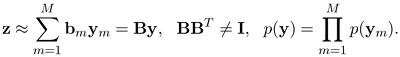
where μ and v define the orientation and scale of the Gabor filter, which is a product of a Gaussian envelope and a complex plane wave with wave vector k_u,v. The family of Gabor filters is self-similar, since all of them are generated from one filter, the mother wavelet, by scaling and rotation via the wave vector k_μ,v. Figure 9.24 depicts 40 commonly used Gabor kernels generalized at five scales and eight orientations with (σ = 2π. For an input image z, its 2D Gabor feature images can be extracted by convoluting z with a Gabor filter, g_μ,_v = z * G_μ,v, where * denotes the convolution operator. Thus, a total of () Gabor feature images g_μ,_v, can be obtained, where and denote the sizes of and respectively.

In [73], all the Gabor images g_μ,v are down-sampled and then concatenated to form an augmented Gabor feature vector representing the input face image. In the sequence, PCA or LDA is applied to the augmented Gabor feature vector for dimensionality reduction and further feature extraction before it is fed to a classifier. Also, it can be seen that due to the similarity between the Gabor filters, there is a great deal of redundancy in the over complete Gabor feature set. To this end, Wiskott et al. [130] proposed to utilize the Gabor features corresponding to some specific facial landmarks, called Gabor jets, instead of the holistic Gabor images. Based on the jet representation, the elastic graph matching (EGM) was then applied for landmark matching and face recognition. The Gabor-based EGM method was one of the top performers in the 1996/1997 FERET competition [95].

Mixture of linear subspaces

Although successful in many circumstances, linear appearance-based methods including the PCA- and LDA-based ones, may fail to deliver good performance when face patterns are subject to large variations in viewpoints, illumination or facial expression, which result in a highly nonconvex and complex distribution of face images. The limited success of these methods should be attributed to their linear nature. A cost-effective approach to address the nonconvex distribution is with a mixture of the linear models. The mixture- or ensemble-based approach embodies the principle of "divide and conquer," by which a complex face recognition problem is decomposed into a set of simpler ones, in each of which a locally linear pattern distribution can be generalized and dealt with by a relatively easy linear solution (see, for example, [93, 114, 38, 15, 75, 39, 77]).

From the designer's point of view, the central issue to the ensemble-based approach is to find an appropriate criterion to decompose the complex face manifold. Existing partition techniques, whether nonparametric clustering such as K-means [48] or model-based clustering such as EM [84], unanimously adopt similarity criterion based on which similar samples are within the same cluster and dissimilar samples are in different clusters. For example, in the view-based representation [93], every face pattern is manually assigned to one of several clusters according to its view angle with each cluster corresponding to a particular view. In the method considered in [114] and [38], the database partitions are automatically implemented using the K-means and EM clustering algorithms respectively. However, although such criterion may be optimal in the sense of approximating real face distribution for tasks such as face reconstruction, face pose estimation, and face detection, they may not be good for the recognition task considered in the section. It is not hard to see that from a classification point of view, the database partition criterion should be aimed to maximize the difference or separability between classes within each "divided" subset or cluster, which as a subproblem then can be relatively easy to "conquer" by a linear face recognition method.

With such a motivation, a novel method of clustering based on separability criterion (CSC) was introduced recently in [75]. Similar to LDA, the separability criterion is optimized in the CSC method by maximizing a widely used separability measure, the between-class scatter (BCS). Let W_k denote the kth cluster, k = [t ... K] with K: the number of clusters. Representing each class Z_i by its mean , the total within-cluster BCS of the training set Z can be defined as

Equation 9.53

where is the center of the cluster W_k. (9.53) implies that a better class-separability intracluster is achieved if S_t has a larger value. The clustering algorithm maximizes S_t by iteratively reassigning those classes whose means have the minimal distances to their own cluster centers so that the separability between classes is enhanced gradually within each cluster. The maximization process can be implemented by the pseudocodes depicted in Figure 9.25.

With the CSC process, the training set Z is partitioned into a set of subsets called maximally separable clusters (MSCs). To take advantage of these MSCs, a two-stage hierarchical classification framework (HCF) was then proposed in [75]. The HCF consists of a group of face recognition subsystems, each one targeting a specific MSC. This is not a difficult task for most traditional face recognition methods such as the YD-LDA [137] used in [75] to work as such a subsystem in a single MSC with limited-sized subjects and high between-class separability.

Nonlinear subspace analysis methods

In addition to the approach using a mixture of locally linear models, another option to generate a representation for nonlinear face manifold is with a globally nonlinear approach. Recently, the so-called kernel machine technique has become one of the most popular tools for designing nonlinear algorithms in the communities of machine learning and pattern recognition [125, 106]. The idea behind the kernel-based learning methods is to construct a nonlinear mapping from the input space (^J) to an implicit high-dimensional feature space () using a kernel function . In the feature space, it is hoped that the distribution of the mapped data is linearized and simplified so that traditional linear methods could perform well. However, the dimensionality of the feature space could be arbitrarily large, possibly infinite. Fortunately, the exact φ(z) is not needed, and the nonlinear mapping can be performed implicitly in ^J by replacing dot products in with a kernel function defined in the input space ^J k(z_i, z_j) = φ(z_i) · φ(z_j). Examples based on such a design include SVMs [125], kernel PCA (KPCA) [107], kernel ICA (KICA) [6], and generalized discriminant analysis (GDA, also known as kernel LDA) [11].

In the kernel PCA [107], the covariance matrix in can be expressed as

Equation 9.54

where is the average of the ensemble in . The KPCA is actually a classic PCA performed in the feature space . Let be the first M most significant eigenvectors of S_cov, and they form a low-dimensional subspace, called KPCA subspace, in . For any face pattern z, its nonlinear principal components can be obtained by the dot product, , computed indirectly through the kernel function k(). When φ(z) = z, KPCA reduces to PCA, and the KPCA subspace is equivalent to the eigenface space introduced in [122].

As such, GDA [11] is used to extract a nonlinear discriminant feature representation by performing a classic LDA in the high-dimensional feature space . However, GDA solves the SSS problem in simply by removing the nullspace of the within-class scatter matrix , although the null space may contain the most significant discriminant information, as mentioned earlier. To this end, a kernel version of LD-LDA [79], also called KDDA, was introduced recently in [78]. In the feature space, the between-class and within-class scatter matrices are given as follows:

Equation 9.55

Equation 9.56

where . Through eigen-analysis of and in the feature space , KDDA finds a low-dimensional discriminant subspace spanned by Θ, an M × N matrix. Any face image z is first nonlinearly transformed to an N x 1 kernel vector,

Equation 9.57

Then, the KDDA-based feature representation y can be obtained by a linear projection: y = Θ · γ(φ(z)).

9.4.3. Pattern classification

Given the feature representation of face objects, a classifier is required to learn a complex decision function to implement final classification. Whereas the feature representation optimized for the best discrimination would help reduce the complexity of the decision function, which is easy for the classifier design, a good classifier would be able to further learn the separability between subjects.

Nearest feature line classifier

The nearest neighbor (NN) is the simplest yet most popular method for template matching. In the NN-based classification, the error rate is determined by the representational capacity of a prototype face database. The representational capacity depends two issues: (1) how the prototypes are chosen to account for possible variations, and (2) how many prototypes are available. However, in practice, only a small number of them are available for a face class, typically from one to about a dozen. It is desirable to have a sufficiently large number of feature points stored to account for as many variations as possible. To this end, Li and Lu [64] proposed a method called the nearest feature line (NFL) to generalize the representational capacity of available prototype images.

The basic assumption behind the NFL method is based on an experimental finding, which revealed that although the images of appearances of the face patterns may vary significantly due to differences in imaging parameters such as lighting, scale, and orientation, these differences have an approximately linear effect when they are small [121]. Consequently, it is reasonable to use a linear model to interpolate and extrapolate the prototype feature points belonging to the same class in a feature space specific to face representation, such as the eigenfaces space. In the simplest case, the linear model is generalized by a feature line (FL) passing through a pair of prototype points (y₁,y₂), as depicted in Figure 9.26. Denoting the FL as , the FL distance between a query feature point y and is defined as

Equation 9.58

where b is y's projection point on the FL, and is a position parameter relative to y₁ and y_2. The FL approximates variants of the two prototypes under variations in illumination and expression (i.e., possible face images derived from the two). It provides a virtually infinite number of prototype feature points of the class. Also, assuming that there are C_i > 1 prototype feature points available for class i, a number of K_i = C_i(C_i – 1)/2 FLs can be constructed to represent the class (e.g., K_i = 10 when C_i = 5). As a result, the representational capacity of the prototype set is significantly enhanced in this way.

The class label (y) of the query feature point y can be inferred by the following NFL rule:

Equation 9.59

The classification results not only determine the class label y, but also provide a quantitative position number ς* as a by-product, which can be used to indicate the relative changes (in illumination and expression) between the query face and the two associated face images y_i*j* = and y_i*k*.

Regularized Bayesian classifier

LDA has its root in the optimal Bayesian classifier. Let P(y = i) and p(z|y = i) be the prior probability of class i and the class-conditional probability density of z given the class label is i respectively. Based on the Bayes formula, we have the following a posteriori probability P(y = i|z), that is, the probability of the class label being i given that z has been measured:

Equation 9.60

The Bayesian decision rule to classify the unlabeled input z is then given as

Equation 9.61

(9.60) is also known as the maximum a posteriori (MAP) rule, and it achieves minimal misclassification risk among all possible decision rules.

The class-conditional densities p(z|y = i) are seldom known. However, often it is reasonable to assume that p(z| y = i) is subjected to a Gaussian distribution. Let μ_i and Σ_i denote the mean and covariance matrix of the class i; we have

Equation 9.62

where is the squared Mahalanobis (quadratic) distance from z to the mean vector μi. With the Gaussian assumption, the classification rule of (9.61) turns to

Equation 9.63

The decision rule of (9.63) produces quadratic boundaries to separate different classes in the J-dimensional real space. Consequently, this is also called quadratic discriminant analysis (QDA). Often, the two statistics (μ_i, Σ_i) are estimated by their sample analogs,

Equation 9.64

LDA can be viewed as a special case of QDA when the covariance structure of all classes are identical (i.e., Σ_i = Σ). However, the estimation for either Σ_i or Σ. is ill-posed in the small sample size (SSS) settings, giving rise to high variance. This problem becomes extremely severe due to C_i ≪ J in face recognition tasks, where Σ_i is singular with rank ≤ (C_i – 1). To deal with such a situation, a regularized QDA, built on the D-LDA idea and Friedman's regularization technique [40], called RD-QDA, was introduced recently in [80]. The purpose of the regularization is to reduce the variance related to the sample-based estimation for the class covariance matrices at the expense of potentially increased bias.

In the RD-QDA method, the face images (z_ij) are first projected into the between-class scatter matrix S_b's complement null subspace spanned by H, obtaining a representation y_ij = H^Tz_ij. The regularized sample covariance matrix estimate of class i in the subspace spanned by H, denoted by , can be expressed as

Equation 9.65

where

Equation 9.66

Equation 9.67

, and (λ, γ) is a pair of regularization parameters. The classification rule of (9.63) then turns to

Equation 9.68

where and π_i = C_i/N is the estimate of the prior probability of class i. The regularization parameter λ (0 ≤ λ ≤ 1) controls the amount that the S_i are shrunk toward S. The other parameter γ (0 ≤ γ ≤ 1) controls shrinkage of the class covariance matrix estimates toward a multiple of the identity matrix. Under the regularization scheme, the classification rule of (9.68) can be performed without experiencing high variance of the sample-based estimation even when the dimensionality of the subspace spanned by H is comparable to the number of available training samples, N.

RD-QDA has a close relationship with a series of traditional discriminant analysis classifiers, such as LDA, QDA, nearest center (NC), and weighted nearest center (WNC). First, the four corners defining the extremes of the (λ, γ) plane represent four well-known classification algorithms, as summarized in Table 9.3, where the prefix D- means that all these methods are developed in the subspace spanned by H derived from the D-LDA technique. Based on Fisher's criterion (9.48) used in YD-LDA [137], it is obvious that the YD-LDA feature extractor followed by an NC classifier is actually a standard LDA classification rule implemented in the subspace H. Also, we have when (λ = 1, γ = η), where and . In this situation, it is not difficult to see that RD-QDA is equivalent to LD-LDA followed by an NC classifier. In addition, a set of intermediate discriminant classifiers between the five traditional ones can be obtained when we smoothly slip the two regularization parameters in their domains. The purpose of RD-QDA is to find the optimal (λ*, γ*) that give the best correct recognition rate for a particular face recognition task.

Table 9.3. A series of discriminant analysis algorithms derived from RD-QDA.

Algs.	D-NC	D-WNC	D-QDA	YD-LDA	LD-LDA
A	1	0	0	1	1
γ	1	1	0	0	η
					α ( + I)

Neural networks classifiers

Linear or quadratic classifiers may fail to deliver good performance when the feature representation y of face images z is subject to a highly nonconvex distribution-for example, in the case depicted in Figure 9.27 (right), where a nonlinear decision boundary much more complex than the quadratic one is required. One option to construct such a boundary is to utilize a neural network classifier. Figure 9.27 (left) depicts the architecture of a general multilayer feedforward neural network (FNN), which consists of one input layer, one hidden layer and one output layer. The input layer has M units to receive the M-dimensional input vector y. The hidden layer is composed of L units, each one operated by a nonlinear activation function h_l(·) to nonlinearly map the input to an L-dimensional space ^L, where the patterns are hoped to become linearly separable, so that linear discriminants can be implemented by the activation function f(·) in the output layer. The process can be summarized as

Equation 9.69

where and are the connecting weights between neighboring layers of units.

The key to the neural networks is to learn the involved parameters. One of the most popular methods is the back-propagation (BP) algorithm based on error gradient descent. The most widely used activation function in both hidden and output units of a BP network is a sigmoidal function given by f(·) = h(·) = t/(1/(1 + e⁽·⁾). Most BP-like algorithms utilize local optimization techniques. As a result, the training results are very much dependent on the choices of initial estimates. Recently, a global FNN learning algorithm was proposed in [120, 119]. The global FNN method was developed by addressing two issues: (1) characterization of global optimality of an FNN learning objective incorporating the weight decay regularizer, and (2) derivation of an efficient search algorithm based on results of (1). The face recognition simulations reported in [120] indicate that the global FNN classifier can perform well in conjunction with various feature extractors, including eigenfaces [122], Fisherfaces [12], and D-LDA [137].

In addition to the classic BP networks, the radial basis function (RBF) neural classifiers have recently attracted extensive interest in the community of pattern recognition. In the RBF networks, the Gaussian function is often preferred as the activation function in the hidden units, , while the output activation function f (·) is usually a linear function. In this way, it can be seen that the output of the RBF networks is actually a mixture of Gaussians. Consequently, it is generally believed that the RBF networks possess the best approximation property. Also, the learning speed of the RBF networks is fast due to locally tuned neurons. Attempts to apply the RBF neural classifiers to solve face recognition problems have been reported recently. For example, in [31], a face recognition system built on an LDA feature extractor and an enhanced RBF neural network produced one of the lowest error rates reported on the ORL face database [2].

Support vector machine classifiers

Assuming that all the examples in the training set Z are drawn from a distribution P(z, y), where y is the label of the example z, the goal of a classifier learning from Z is to find a function f(z, α*) to minimize the expected risk:

Equation 9.70

where α is a set of abstract parameters. Since P(z, y) is unknown, most traditional classifiers, such as nearest neighbor, Bayesian classifier, and neural network, solve the specific learning problem using the so-called empirical risk (i.e., training error) minimization (ERM) induction principle, where the expected risk function R(α) is replaced by the empirical risk function: . As a result, the classifiers obtained may be entirely unsuitable for classification of unseen test patterns, although they may achieve the lowest training error. To this end, Vapnik and Chervonenkis [126] provide a bound on the deviation of the empirical risk from the expected risk. The bound, also called Vapnik-Chervonenkis (VC) bound, holding with probability (1 -η), has the following form:

Equation 9.71

where h is the VC-dimension as a standard measure to the complexity of the function space that f(z_i, α) is chosen from. It can be seen from the VC bound that both R_emp(α) and (h/N) have to be small to achieve good generalization performance.

Based on the VC theory, the SVMs embody the structural risk minimization principle, which aims to minimize the VC bound. However, often it is intractable to estimate the VC dimension of a function space. Fortunately, it has been shown in [125] that for the function class of hyperplanes, f(z) = w · z + b, its VC dimension can be controlled by increasing the margin, which is defined as the minimal distance of an example to the decision surface (see Figure 9.28). The main idea behind SVMs is to find a separating hyperplane with the largest margin, as shown in Figure 9.28, where the margin is equal to 2/ ||w||.

For a binary classification problem where y_i ∊ {1, –1}, the general optimal separating hyperplane sought by SVM is the one that

Equation 9.72

subject to y_i(w^Tz_i + b) ≥ 1 – ξ_i, ξ_i ≥ 0, where ξ_i are slack variables, ζ is a regularization constant, and the hyperplane is defined by parameters w and b. After some transformations, the minimization in (9.72) can be reformulated as

Equation 9.73

subject to 0 ≤ α_i ≤ ζ and , where α_i are positive Lagrange multipliers. Then, the solution, and b* = y_i – w* · z_i(), can be derived from (9.73) using quadratic programming. The support vectors are those examples (z_i, y_i) with .

For a new data point z, the classification is performed by a decision function,

Equation 9.74

In the case where the decision function is not a linear function of the data, SVMs first map the input vector z into a high-dimensional feature space by a nonlinear function φ (z), and then construct an optimal separating hyperplane in the high-dimensional space with linear properties. The mapping φ (z) is implemented using kernel machine techniques, as it is done in KPCA and GDA. Examples of applying SVMs into the face recognition tasks can be found in [94, 56, 47, 76].

9.4.4. Evaluation

In this section, we introduce several experiments from our recent studies on subspace analysis methods. Following standard face recognition practices, any evaluation database (G) used here is randomly partitioned into two subsets: the training set Z and the test set Q. The training set consists of images: C_i images per subject are randomly chosen. The remaining images are used to form the test set Q = G − Z. Any face recognition method evaluated here is first trained with Z, and the resulting face recognizer is then applied to Q to obtain a correct recognition rate (CRR), which is defined as the fraction of the test examples correctly classified. To enhance the accuracy of the assessment, all the CRRs reported here are averaged over ≥ 5 runs. Each run is executed on a random partition of the database G into Z and Q.

Linear and quadratic subspace analysis

The experiment is designed to assess the performance of various linear and quadratic subspace analysis methods, including eigenfaces, YD-LDA, LD-LDA, RD-QDA, and those listed in Table 9.3. The evaluation database used in the experiment is a midsized subset of the FERET database. The subset consists of 606 grayscale images of 49 subjects, each one having more than 10 samples. The performance is evaluated in terms of the CRR and the sensitivity of the CRR measure to the SSS problem, which depends on the number of training examples per subject C_i. To this end, six tests were performed with various values of C_i ranging from C_i = 2 to C_i = 7.

The CRRs obtained by RD-QDA in the (λ, γ) grid are depicted in Figure 9.29. Also, a quantitative comparison of the best found CRRs and their corresponding parameters among the seven methods is summarized in Table 9.4. The parameter λ controls the degree of shrinkage of the individual class covariance matrix estimates S_i toward the within-class scatter matrix, (H^TS_WH). Varying the values of λ within [0,1] leads to a set of intermediate classifiers between D-QDA and YD-LDA. In theory, D-QDA should be the best performer among the methods evaluated here if sufficient training samples are available. It can be observed at this point from Figure 9.29 that the CRR peaks gradually moved from the central area toward the corner (0, 0); that is the case of D-QDA as C_i increases. Small values of A have been good enough for the regularization requirement in many cases (C_i ≥ 3). However, both D-QDA and YD-LDA performed poorly when C_i = 2. This should be attributed to the high variance of the estimates of S_i and S due to insufficient training samples. In this case, Si and even S are singular or close to singular, and the resulting effect is to dramatically exaggerate the importance associated with the eigenvectors corresponding to the smallest eigenvalues. Against the effect, the introduction of another parameter γ helps to decrease the larger eigenvalues and increase the smaller ones, thereby counteracting to some extent the bias. This is also why LD-LDA greatly outperformed YD-LDA when C_i = 2. Although LD-LDA seems to be a little overregularized compared to the optimal RD-QDA(λ*, γ*), the method almost guarantees a stable suboptimal solution. A CRR difference of 4.5% on average over the range C_i ∊ [2, 7] has been observed between the top performer RD-QDA(λ*, γ*) and LD-LDA. It can be concluded, therefore, that LD-LDA should be preferred when insufficient prior information about the training samples is available and a cost-effective processing method is sought.

Table 9.4. Comparison of correct recognition rates (CRRs) (%).

Ci =	2	3	4	5	6	7
Eigenfaces	59.8	67.8	73.0	75.8	81.3	83.7
D-NC	67.8	72.3	75.3	77.3	80.2	80.5
D-WNC	46.9	61.7	68.7	72.1	73.9	75.6
D-QDA	57.0	79.3	87.2	89.2	92.4	93.8
YD-LDA	37.8	79.5	87.8	89.5	92.4	93.5
LD-LDA (η)	70.7 0.84	77.4 0.75	82.8 0.69	85.7 0.65	88.1 0.61	89.4 0.59
RD-QDA (λ*) (γ*)	73.2 0.93 0.47	8I.6 0.93 0.10	88.5 0.35 0.07	90.4 0.11 0.01	93.2 0.26 le-4	94.4 0.07 le-4

In addition to the regularization, it is found that the performance of the LDA-based methods can be further improved with an ensemble-based approach [75]. The approach uses cluster analysis techniques like the K-mean and the CSC method mentioned earlier to form a mixture of LDA subspaces. Experiments conducted on a compound database with 1654 face images of 157 subjects and a large FERET subset with 2400 face images of 1200 subjects indicate that the performance of both YD-LDA and LD-LDA can be greatly enhanced under the ensemble framework. The average CRR improvement that has been observed so far ranges from 6% to 22%.

Nonlinear subspace analysis

Applications of kernel-based methods in face research have been widely reported (e.g., [69, 63, 58, 134, 78, 62]). Here, we introduce two experiments to illustrate the effectiveness of the kernel-based discriminant analysis methods in face recognition tasks. The two experiments were conducted on a multiview face database, the UMIST database [46], consisting of 575 images of 20 people, each covering a wide range of poses from profile to frontal views.

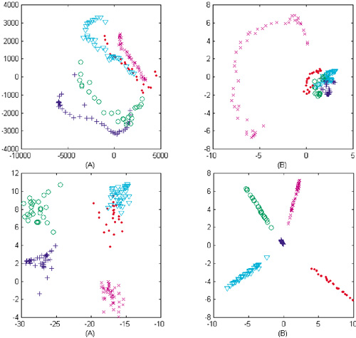
The first experiment provided insights on the distribution of face pattern in four types of subspaces generalized by utilizing the PCA [122], KPCA [107], LD-LDA [79], and KDDA [78] algorithms respectively. The projections of five face subjects in the first two most significant feature bases of each sub-space are shown in Figure 9.30. Figure 9.30 (upper) shows the first two most significant principal components extracted by PCA and KPCA, and they provide a low-dimensional representation for the samples in a least-square sense. Thus we can roughly learn the original distribution of the samples from Figure 9.30 (upper A), where it can been seen that the distribution is as expected nonconvex and complex. Also, it is hard to find any useful improvement in Figure 9.30 (upper B) for the purpose of pattern classification. Figure 9.30 depicts the first two most discriminant features extracted by LD-LDA and KDDA respectively. Obviously, these features outperform, in terms of discriminant power, those obtained by using the PCA-like techniques. However, subject to limitation of linearity, some classes are still nonseparable in Figure 9.30 (lower A). In contrast to this, we can see the linearization property of the KDDA-based subspace, as shown in Figure 9.30 (lower B), where all of the classes are well linearly separable.

The second experiment compares the CRR performance among the three kernel-based methods, KPCA [107], GDA (also called KDA) [11], and KDDA [78]. The two most popular face recognition algorithms, eigenfaces [122] and Fisherfaces [12], were also implemented to provide performance baselines. C_i = 6 images per person were randomly chosen to form the training set Z. The nearest neighbor was chosen as the classifier following these feature extractors. The obtained results with best found parameters are depicted in Figure 9.31, where KDDA is clearly the top performer among all the methods evaluated here. Also, it can be observed that the performance of KDDA is more stable and predictable than that of GDA. This should be attributed to the introduction of the regularization, which significantly reduces the variance of the estimates of the scatter matrices arising from the SSS problem.

Other performance evaluations

Often, it is desired in the face recognition community to give the overall evaluation and benchmarking of various face recognition algorithms. Here, we introduce several recent face recognition evaluation reports in literature. Before we proceed to an evaluation, it should be noted that the performance of a learning-based pattern recognition system is very data- and application-dependent, and there is no theory that can accurately predict them for unknown distribution data/new applications. In other words, some methods that have reported almost perfect performance in certain scenarios may fail in other scenarios.

To date, the FERET program incepted in 1993 has made a significant contribution to the evaluation research of face recognition algorithms by building the FERET database and the evaluation protocol [3, 96, 95]. Their availability has made it possible to objectively assess the laboratory algorithms under close to real-world conditions. In the FERET protocol, an algorithm is given two sets of images: the target set and the query set. The target set is a set of known facial images, while the query set consists of unknown facial images to be identified. Furthermore, multiple galleries and probe sets can be constructed from the target and query sets respectively. For a pair of given gallery G and probe set P, the CRR is computed by examining the similarity between the two sets of images. Table 9.5 depicts some test results reported in the September 1996 FERET evaluation [95]. B-PCA and B-Corr are two baseline methods based on PCA and normalized correlation [122, 88]. D-eigenfaces is the dual eigenfaces method [86]. LDA.M [115] and LDA.U1/U2 [33, 141] are three LDA-based algorithms. GrayProj is a method using grayscale projection [129]. EGM-GJ is the elastic graph matching method with Gabor jet [130]. X denotes an unknown algorithm from Excalibur Corporation. It can be seen that among these evaluated methods, D-eigenfaces, LDA.U2, and EGM-GJ are the three top performers. Based on the FERET program, the face recognition vendor tests (FRVTs) that systematically measured commercial face recognition products were also developed, and the latest FRVT 2002 reports can be found in [1].

Table 9.5. CRR performance rank of algorithms in the September 1996 FERET evaluation [95].

Algorithms	on FB Probes						on Duplicate I Probes
	G1	G2	G3	G4	G5	G6	G1	G2	G3	G4	G5
B-PCA	9	10	8	8	10	8	6	10	5	5	9
B-Corr	9	9	9	6	9	10	10	7	6	6	8
X	6	7	7	5	7	6	3	5	4	4	3
Eigenfaces	4	2	1	1	3	3	2	1	2	2	3
D-Eigenfaces	7	5	4	4	5	7	7	4	7	8	10
LDA.M	3	4	5	8	4	4	9	6	8	10	6
GrayProj	7	8	9	6	7	9	5	7	10	7	6
LDA.U1	4	6	6	10	5	5	7	9	9	9	3
LDA.U2	1	1	3	2	2	1	4	2	3	3	1
EGM-GJ	2	3	2	2	1	1	1	3	1	1	1

Recently, Moghaddam [85] evaluated several unsupervised subspace analysis methods and showed that dual PCA (dual eigenfaces) > KPCA > PCA ≈ ICA, where > denotes "outperform" in terms of the average CRR measure. Compared to these unsupervised methods, it is generally believed that algorithms based on LDA are superior in face recognition tasks. However, it is shown recently in [83] that this is not always the case. PCA may outperform LDA when the number of training samples per subject is small or when the training data nonuniformly sample the underlying distribution. Also, PCA is shown to be less sensitive to different training data sets. More recent evaluation results of subspace analysis methods in different scenarios can be found in Table 9.6, where LDA is based on the version of [33, 12], PPCA is the probabilistic PCA [118], and KICA is the kernel version of ICA [6]. The overall performance of linear subspace analysis methods was summarized as LDA > PPCA > PCA > ICA, and it was also observed that kernel-based methods are not necessarily better than linear methods [62].

Table 9.6. CRR performance rank of subspace methods in [62].

Rank	1	2	3	4	5	6	7
Pose	KDA	PCA	KPCA	LDA	KICA	ICA	PPCA
Expression	KDA	LDA	PPCA	PCA	KPCA	ICA	KICA
Illumination	LDA	PPCA	KDA	KPCA	KICA	PCA	ICA

Acknowledgments

Portions of the research in this chapter use the FERET database of facial images collected under the FERET program [96]. The authors would like to thank the FERET Technical Agent, the U.S. National Institute of Standards and Technology (NIST), for providing the FERET database.