6.2. Advanced Image-Based Lighting

The technique of image-based lighting can be used not only to illuminate synthetic objects with real-world light, but to place synthetic objects into a real-world scene. To do this realistically, the objects need to photometrically affect their environment; that is, they need to cast shadows and reflect indirect illumination onto their nearby surroundings. Without these effects, the synthetic object will most likely look "pasted in" to the scene rather than as if it had actually been there.

A limitation of the techniques presented so far is that they require that the series of digital images taken span the complete range of intensities in the scene. For most scenes, the range of shutter speeds available on a digital camera can cover this range effectively. However, for sunlit scenes, the directly visible sun is often too bright to capture, even using the shortest exposure times available. This is a problem, since failing to record the color and intensity of the sun will cause significant inaccuracies in the captured lighting environment.

This section describes extensions to the image-based lighting techniques that solve both the problem of capturing the intensity of the sun and the problem of having the synthetic objects cast shadows onto the environment.

Although presented together, they are independent techniques that can be used separately as needed. These techniques are presented in the form of a new image-based lighting example, also using the RADIANCE rendering system.

6.2.1. Capturing a light probe in direct sunlight

For our example, we place a new sculpture and some spheres in front of the Guggenheim Museum in Bilbao, Spain, seen in Figure 6.9a. To create this example, I first photographed a background plate image using a Canon EOS-D60 digital camera on a tripod, as in Figure 6.9b. The image was taken with a 24mm lens at ASA 100 sensitivity, f/11 aperture, and 1/60 second shutter speed. A shadow from a nearby lamppost can be seen being cast along the ground.

To capture the lighting, I placed a three-inch mirrored sphere on a second tripod in front of the camera, as in Figure 6.10. I left the first camera in the same place, pointing in the same direction, since that would make it easier to align the probe and background images later. In order to keep the reflection of the camera small in the sphere, I placed the sphere approximately one meter away from the camera, and then changed to a 200mm telephoto lens in order for the sphere to appear relatively large in the frame. I used a remote release for the camera shutter to avoid moving the camera while capturing the lighting, and I took advantage of the camera's automatic exposure bracketing (AEB) feature to quickly shoot the mirrored sphere at 1/60, 1/250, and 1/1000 second. These images are shown in Figure 6.11a-c. The images were recorded using the camera's "RAW" mode, which saves uncompressed image data to the camera's memory card. This ensures capturing the best possible image quality and for this camera has the desirable effect that the image pixel values exhibit a linear response to incident light in this mode. Knowing that the response is linear is helpful for assembling high dynamic range images, since there is no need to derive the response curve of the camera.

Since the sun was shining, it appears in the reflection in the mirrored sphere as seen by the camera. Because the sun is so bright, even the shortest 1/1000 second exposure failed to capture the sun's intensity without saturating the image sensor. After assembling the three images into a high dynamic range image, the area near the sun was not recorded properly, as seen in Figure 6-11d. As a result, using this image as a lighting environment would produce mismatched lighting, since a major source of the illumination would not have been accounted for.

I could have tried using several techniques to record an image of the mirrored sphere such that the sun did not saturate. I could have taken an even shorter exposure at 1/4000 second (the shortest shutter speed available on the camera), but it's almost certain the sun would still be too bright. I could have made the aperture smaller, taking the picture at f/22 or f/32 instead of f/11, but this would change the optical properties of the lens, and it would be unlikely to be a precise ratio of exposure to the previous images. Also, camera lenses tend to produce their best images at f/8 or f/11. I could have placed a neutral density filter in front of the lens, but this would also change the optical properties of the lens (the resulting image might not line up with the others due to refraction or from bumping the camera). Instead, I used a technique that allows us to indirectly measure the intensity of the sun, which is to photograph a diffuse gray sphere in the same location (Figure 6.12).

The image of the diffuse gray sphere allows us to reconstruct the intensity of the sun in the following way. Suppose that we had actually been able to capture the correct color and intensity of the sun in the light probe image. Then, if we were to use that light probe image to illuminate a synthetic diffuse gray sphere, it should have the same appearance as the real gray sphere actually illuminated by the lighting environment. However, since the light probe failed to record the complete intensity of the sun, the rendered diffuse sphere will not match the real diffuse sphere, and in fact we would expect it to be significantly darker. As we will see, the amount by which the rendered sphere is darker in each of the three color channels tells us the correct color and intensity for the sun.

The first part of this process is to make sure that all of the images that have been taken are radiometrically consistent. So far, we've recorded light in three different ways: seen directly with the 24mm lens, seen reflected in the mirrored sphere through the 200mm lens, and as reflected off of the diffuse sphere with the 200mm lens. Although the 24mm and 200mm lenses were both set to an f/11 aperture, they did not necessarily transmit the same amount of light to the image sensor. To measure this difference, we can photograph a white spot of light in our laboratory with the cameras to determine the transmission ratio between the two lenses at these two f/stops, as seen in Figure 6.13. The measurement recorded that the spot in the 24mm lens image appeared 1.42 times as bright in the red channel, 1.40 times as bright in green, and 1.38 times as bright in blue compared to the 200mm lens image. Using these results, we can multiply the pixel values of the images acquired with the 200mm lens by (1.42, 1.40, 1.38) so that the images represent places in the scene with equal colors and intensities equally. I could have been even more precise by measuring the relative amount of light transmitted as a spatially varying function across each lens, perhaps by photographing the spot in different places in the field of view of each lens. At wider f/stops, many lenses, particularly wide-angle ones, transmit significantly less light to the corners of the image than to the center. Since the f/11 f/stop was reasonably small, I made the assumption that these effects would not be significant.

Continuing toward the goal of radiometric consistency, we should note that neither the mirrored sphere nor the diffuse sphere are 100% reflective. The diffuse sphere is intentionally painted gray instead of white so that it is less likely to saturate the image sensor if an automatic light meter is employed. I measured the paint's reflectivity by painting a flat surface with the same color, and then photographing the surface in diffuse natural illumination. In the scene, I also placed a similarly oriented reflectance standard, a white disk of material specially designed to reflect nearly 100% of all wavelengths of light across the visible spectrum. By dividing the average RGB pixel value of the painted sample to average pixel value of the reflectance standard, I determined that the reflectivity of the gray paint was (0.032, 0.333, 0.346) in the red, green, and blue channels. By dividing the pixel values of the gray sphere image by these values, I obtained an image of how a perfectly white sphere would have appeared in the lighting environment. Reflectance standards such as the one that I used are available from companies such as Coastal Optics and LabSphere. A less expensive solution is to use the white patch of a MacBeth ColorChecker chart. We have measured the white patch of the chart to be 86% reflective, so any measurement taken with respect to this patch should be multiplied by 0.86 to scale it to be proportional to absolute reflectance.

The mirrored sphere is also not 100% reflective; even specially made first-surface mirrors are rarely greater than 90% reflective. To measure the reflectivity of the sphere to first order, I photographed the sphere on a tripod with the reflectance standard facing the sphere in a manner such that both the standard and its reflection were visible in the same frame, as in Figure 6.14. Dividing the reflected color by the original color revealed that the sphere's reflectivity was (0.632, 0.647, 0.653) in the red, green, and blue channels. Using this measurement, I further scaled the pixel values of the image of the mirrored sphere in Figure 6.11 by () to approximate the image that a perfectly reflective sphere would have produced.

To be more precise, I could have measured and compensated for the sphere's variance in reflectivity with the angle of incident illumination. Due to the Fresnel reflection effect, the sphere will exhibit greater reflection toward grazing angles. However, my group has measured that this effect is less than a few percent for all measurable angles of incidence of the spheres we have used so far.

Now that the images of the background plate, the mirrored sphere, and the diffuse sphere have been mapped into the same radiometric space, we need to model the missing element, which is the sun. The sun is 1,390,000 km in diameter and on average 149,600,000 km away, making it appear as a disk in our sky with a subtended angle of 0.53 degrees. The direction of the sun could be calculated from standard formulas involving time and geographic coordinates, but it can also be estimated reasonably well from the position of the saturated region in the mirrored sphere. If we consider the mirrored sphere to have image coordinates (u, v) each ranging from –1 to 1, a unit vector (D_x, D_y, D_z) pointing toward the faraway point reflected toward the camera at (u, v) can be computed as

Equation 6.1

Equation 6.2

Equation 6.3

In this case, the center of the saturated image was observed at coordinate (0.414, 0.110) yielding a direction vector of (0.748, 0.199, 0.633). Knowing the sun's size and direction, we can now model the sun in RADIANCE as an infinite source light:

We have not yet determined the radiance of the sun disk, so in this file sun.rad, I chose its radiance L to be (46700, 46700, 46700). This radiance value happens to be such that the brightest point of a diffuse white sphere lit by this environment will reflect a radiance value of (1, 1, 1). To derive this number, I computed the radiance L_r of the point of the sphere pointing toward the sun based on the rendering equation for Lambertian diffuse reflection [6]:

Since the radius of our 0.53° diameter sun is r = 0.00465 radians, the range of θ is small enough to approximate sin θ ≈ θ and cos θ ≈ 1, yielding

Letting our desired radiance from the sphere be L_r = 1 and its diffuse reflectance to be a perfect white ρ_d = 1, we obtain that the required radiance value L for the sun is 1/r² = 46700. A moderately interesting fact is that this tells us that on a sunny day, the sun is generally over 46,700 times as bright as the sunlit surfaces around you. Knowing this, it is not surprising that it is difficult to capture the sun's intensity with a camera designed to photograph people and places.

Now we are set to compute the correct intensity of the sun. Let us call our incomplete light probe image (the one that failed to record the intensity of the sun) P_incomplete. If we render an image of a virtual mirrored sphere illuminated by only the sun, we obtain a synthetic light probe image of the synthetic sun. Let us call this probe image P_sun. The desired complete light probe image, P_complete, can thus be written as the incomplete light probe plus some color α = (α_r, α_g, α_b) times the sun light probe image, as in Figure 6.15.

To determine P_comlpete, we somehow need to solve for the unknown α. Let us consider, for each of the three light probe images, the image of a diffuse white sphere as it would appear under each of these lighting environments, which we can call D_complete, D_incomplete, and D_sun. We can compute D_incomplete by illuminating a diffuse white sphere with the light probe image P_incomplete using the image-based lighting technique from the previous section. We can compute D_sun by illuminating a diffuse white sphere with the unit sun specified in sun.rad from Table 6.7. Finally, we can take D_complete to be the image of the real diffuse sphere under the complete lighting environment. Since lighting objects is a linear operation, the same mathematical relationship for the light probe images must hold for the images of the diffuse spheres they are illuminating. This gives us the equation illustrated in Figure 6.16.

# sun.rad
void light suncolor 0 0 3 46700 46700 46700
suncolor source sun 0 0 4 0.748 0.199 0.633 0.53

We can now subtract D_incomplete from both sides to obtain the equation in Figure 6.17.

Since D_sun and D_complete – D_incomplete are images consisting of thousands of pixel values, the equation in Figure 6.17 is actually a heavily overdeter-mined set of linear equations in α, with one equation resulting from each red, green, and blue pixel value in the images. Since the shadowed pixels in D_sun are zero, we cannot just divide both sides by D_sun to obtain an image with an average value of α. Instead, we can solve for α in a least squares sense to minimize α D_sun - (D_complete - D_incomplete). In practice, however, we can more simply choose an illuminated region of D_sun, take this region's average value μ_sun, then take the same region of D_complete - D_incomplete, compute its average pixel value μdiff, and then compute a = μdiff/μ_sun.

Applying this procedure to the diffuse and mirrored sphere images from Bilbao, I determined α = (1.166, 0.973, 0.701). Multiplying the original sun radiance (46700, 46700, 46700) by this number, we obtain (54500, 45400, 32700) for the sun radiance, and we can update the sun.rad from Table 6.7 accordingly.

We can now verify that the recovered sun radiance has been modeled accurately by lighting a diffuse sphere with the sum of the recovered sun and the incomplete light probe P_incomplete. The easiest way to do this is to include both the sun. rad environment and the light probe image together as the RADIANCE lighting environment. Figure 6.18a and b show a comparison between such a rendering and the actual image of the diffuse sphere.

Subtracting the two images allows us to visually verify the accuracy of the lighting reconstruction. The difference image in Figure 6.18c is nearly black, which indicates a close match.

The rendered sphere in Figure 6.18b is actually illuminated with a combination of the incomplete light probe image and the modeled sun light source rather than with a complete image-based lighting environment. To obtain a complete light probe, we can compute P_complete = P_incomplete + α P_sun as above and use this image on its own as the light probe image. However, it is actually advantageous to keep the sun separate as a computer-generated light source rather than as part of the image-based lighting environment. The reason for this has to do with how efficiently the Monte Carlo rendering system can generate the renderings. As seen in Figure 6.6, when a camera ray hits a point on a surface in the scene, a multitude of randomized indirect illumination rays are sent into the image-based lighting environment to sample the incident illumination. Since the tiny sun disk occupies barely 1/100000 of the sky, it is unlikely that any of the rays will hit the sun even if 1000 or more rays are traced to sample the illumination. Any such point will be shaded incorrectly as if it is in shadow. What is worse is that for some of the points in the scene at least one of the rays fired out will hit the sun. If 1000 rays are fired and one hits the sun, the rendering algorithm will light the surface with the sun's light as if it were 1/1000 of the sky, which is 100 times as large as the sun actually is. The result is that every 100 or so pixels in the render there will be a pixel that is approximately 100 times as bright as it should be, and the resulting rendering will appear very "speckled."

Leaving the sun as a traditional computer-generated light source avoids this problem almost entirely. The sun is still in the right place with the correct size, color, and intensity, but the rendering algorithm knows explicitly that it is there. As a result, the sun's illumination will be computed as part of the direct illumination calculation: for every point of every surface, the renderer will always fire at least one ray toward the sun. The renderer will still send a multitude of indirect illumination rays to sample the sky, but since the sky is relatively uniform, its illumination contribution can be sampled sufficiently accurately with a few hundred rays. (If any of the indirect illumination rays do hit the sun, they will not add to the illumination of the pixel, since the sun's contribution is already being considered in the direct calculation.) The result is that renderings with low noise can be computed with a small fraction of the rays that would otherwise be necessary if the sun were represented as part of the image-based lighting environment.

The technique of representing a concentrated image-based area of illumination as a traditional CG light source can be extended to multiple light sources within more complex lighting environments. Section 6.2.3 describes how the windows and ceiling lamps within St. Peter's Basilica were modeled as local area lights to efficiently render the animation Fiat Lux. Techniques have also been developed to approximate image-based lighting environments entirely as clusters of traditional point light sources [5, 17, 2]. These algorithms let the user specify the desired number of light sources and then use clustering algorithms to choose the light source positions and intensities to best approximate the lighting environment. Such techniques can make it possible to simulate image-based lighting effects using more traditional rendering systems.

At this point, we have successfully recorded a light probe in a scene where the sun is directly visible; in the next section, we use this recorded illumination to realistically place some new objects in front of the museum.

6.2.2. Compositing objects into the scene including shadows

The next step of rendering the synthetic objects into the scene involves reconstructing the scene's viewpoint and geometry rather than its illumination. We first need to obtain a good estimate of the position, orientation, and focal length of the camera at the time that it photographed the background plate image. Then, we must create a basic 3D model of the scene that includes the surfaces with which the new objects will photometrically interact—in our case, this is the ground plane upon which the objects will sit.

Determining the camera pose and local scene geometry could be done through manual survey at the time of the shoot or through trial and error afterwards. For architectural scenes such as ours, it is usually possible to obtain these measurements through photogrammetry, often from just the one background photograph. Figure 6.19 shows the use of the Façade photogrammetric modeling system described in [12] to reconstruct the camera pose and the local scene geometry based on a set of user-marked edge features in the scene.

The objects we place in front of the museum are a statue of a Caryatid from the Athenian Acropolis and four spheres of differing materials: silver, glass, plaster, and onyx. By using the recovered camera pose, we can render these objects from the appropriate viewpoint, and using the light probe image, we can illuminate the objects with the lighting from the actual scene. However, overlaying such rendered objects onto the background plate image will not result in a realistic image, since the objects would not photometrically interact with the scene: the objects would not cast shadows on the ground, the scene would not reflect in the mirrored sphere or refract through the glass one, and there would be no light reflected between the objects and their local environment.

To have the scene and the objects appear to photometrically interact, we can model the scene in terms of its approximate geometry and reflectance and add this model of the scene to participate in the illumination calculations along with the objects. The ideal property for this approximate scene model to have is for it to precisely resemble the background plate image when viewed from the recovered camera position and illuminated by the captured illumination. We can achieve this property easily if we choose the model's geometry to be a rough geometric model of the scene, projectively texture-mapped with the original background plate image. Projective texture mapping is the image-based rendering process of assigning surface colors as if the image were being projected onto the scene as if from a virtual slide projector placed at the original camera position. Since we have recovered the camera position, performing this mapping is a straightforward process in many rendering systems. A useful property of projective texture mapping is that when an image is projected onto geometry, a rendering of the scene looks just like the original image when viewed from the same viewpoint as the projection. When viewed from different viewpoints, the similarity between the rendered viewpoint the original scene is a function of how far the camera has moved and the accuracy of the scene geometry. Figure 6.20 shows a bird's-eye view of the background plate projected onto a horizontal polygon for the ground plane and a vertical polygon representing the museum in the distance; the positions of these two polygons were determined from the photogrammetric modeling step in Figure 6.19.

When a texture map is applied to a surface, the renderer can be told to treat the texture map's pixel values either as measures of the surface's radiance, or as measures of the surface's reflectance. If we choose to map the values on as radiance, then the surface is treated as an emissive surface that appears precisely the same no matter how it is illuminated or what sort of objects are placed in its vicinity. This is in fact how we have been mapping the light probe images onto the sky dome as the "glow" material to become image-based lighting environments. However, for the ground beneath the objects, this is not the behavior we want. We instead need to texture-map the ground plane with reflectance values, which allows the ground plane to participate in the same illumination computation as the added objects, thus allowing the ground plane to receive shadows and interreflect light with the objects. In RADIANCE, we can do this by specifying the material as "plastic" with no specular component and then modulating the diffuse color values of the surface using the projective texture map.

The problem we now face is that the pixels of the background plate image are actually measurements of radiance—the amount light reflecting from the scene toward the camera—rather than reflectance, which is what we need to project onto the local scene. Reflectance values represent the proportion of incident light that a surface reflects back (also known as the material's albedo) and range from zero (0% of the light is reflected) to one (100% of the light is reflected). Considered in RGB for the three color channels, these reflectance values represent what we traditionally think of as the inherent "color" of a surface, since they are independent of the incident illumination. Radiance values are different in that they can range from zero to arbitrarily high values. Thus, it is generally inaccurate to use radiance values as if they were reflectance values.

As it turns out, we can convert the radiance values from the background plate image into reflectance values using the following relationship:

or

Since the background plate image tells us the radiance for each point on the local scene, all we need to know is the irradiance of each point as well. These irradiance values can be determined using the illumination that we recorded within the environment in the following manner. We assign the local scene surfaces a diffuse material property of known reflectance, for example, 50% gray, or (0.5, 0.5, 0.5) in RGB. We then render this local scene as illuminated by the image-based lighting environment to compute the appearance of the scene under the lighting, seen in Figure 6.21a. With this rendering, we can determine the irradiance of each surface point at irradiance = radiance/reflectance, where the reflectance is the 50% gray color. Finally, we can compute the reflectance, or albedo map, of the local scene as reflectance = radiance/irradiance, where the radiance values are the pixel values from the background plate. The result of this division is shown in Figure 6.21b.

In the renderings in Figure 6.21, I kept the billboard polygon for the building mapped with the original scene radiance from the background plate, rather than attempting to estimate its reflectance values. The main reason I made this choice is that for the objects I would be placing in the scene, their photometric effect on the building in the background did not seem likely to be visually significant.

In this example, the local scene is a single polygon, and thus no point of the local scene is visible to any other point. As a result, it really makes no difference what reflectance value we assume for the scene when we compute its irradiance. However, if the local scene were a more complicated, nonconvex shape, such as we would see on a flight of stairs, the surfaces of the local scene would interreflect. Thus, the reflectance value chosen for computing the irrradiance will affect the final reflectance values solved for by the algorithm. For this reason, it makes sense to try to choose an approximately correct value for the assumed reflectance; 50% gray is more likely to be accurate than 100% reflective. If better accuracy in determining the local scene reflectance is desired, then the reflectance estimation process could be iterated using the reflectance computed by each stage of the algorithm as the assumed reflectance in the next stage. A similar approach to the problem of estimating local scene reflectance is described in [7]. By construction, the local scene with its estimated reflectance properties produces precisely the appearance found in the background plate when illuminated by the recovered lighting environment.

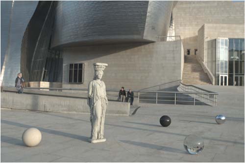
At this point, it is a simple process to create the final rendering of the objects added in to the scene. We include the synthetic objects along with the local scene geometry and reflectance properties, and ask the renderer to produce a rendering of the scene as illuminated by the recovered lighting environment. This rendering for our example can be seen in Figure 6.22, using two bounces of indirect illumination. In this rendering, the objects are illuminated consistently with the original scene, they cast shadows in the appropriate direction, and their shadows are the appropriate color. The scene reflects realistically in the shiny objects and refracts realistically through the translucent objects. If all of the steps were followed for modeling the scene's geometry, photometry, and reflectance, the synthetic objects should look almost exactly as they would if they were really there in the scene.

6.2.3. Image-based lighting in Fiat Lux

The animation Fiat Lux shown at the SIGGRAPH 99 Electronic Theater used image-based lighting to place synthetic monoliths and spheres into the interior of St. Peter's Basilica. A frame from the film is shown in Figure 6.25. The project required making several extensions to the image-based lighting process to handle an interior environment with many concentrated light sources.

The source images for the St. Peter's sequences in the film were acquired on location with a Kodak DCS-520 camera. Each image was shot in high dynamic range at the following exposures: 2 sec, 1/4 sec, 1/30 sec, 1/250 sec, 1/1000 sec, and 1/8000 sec. The images consisted of 10 light probe images taken using a mirrored sphere along the nave and around the altar, and two partial panoramic image mosaics to be used as the background plate images (one is shown in Figure 6.24a).

The film not only required adding synthetic animated objects into the Basilica, but it also required rotating and translating the virtual camera. To accomplish this, we used the Façade system to create a basic 3D model of the interior of the Basilica from one of the panoramic photographs, shown in Figure 6.23. Projecting the panoramic image onto the 3D model allowed novel viewpoints of the scene to be rendered within several meters of the original camera position.

Projecting the HDR panoramic image onto the Basilica's geometry caused the illumination of the environment to emanate from the local geometry rather than from infinitely far away, as seen in other IBL examples. As a result, the illumination from the lights in the vaulting and the daylight from the windows comes from different directions, depending on where a synthetic object in the model is placed. For each panoramic environment, the lighting was derived using a combination of the illumination within each HDR panorama as well as light probe images to fill in areas not seen in the partial panoramas.

As in the Bilbao example, the image-based lighting environment was used to solve for the reflectance properties of the floor of the scene so that it could participate in the lighting computation. A difference is that the marble floor of the Basilica is rather shiny, and significant reflections from the windows and light sources were present within the background plate. In theory, these shiny areas could have been computationally eliminated using the knowledge of the lighting environment. Instead, though, we decided to remove the specularities and recreate the texture of the floor using an image editing program. Then, after the diffuse albedo of the floor was estimated using the reflectometry technique from the last section, we synthetically added a specular component to the floor surface. For artistic reasons, we recreated the specular component as a perfectly sharp reflection with no roughness, virtually polishing the floor of the Basilica.

To achieve more efficient renderings, we employed a technique of converting concentrated sources in the incident illumination images into computer-generated area light sources. This technique is similar to how the sun was represented in our earlier Bilbao example, although there was no need to indirectly solve for the light source intensities, since even the brightest light sources fell within the range of the HDR images. The technique for modeling the light sources was semiautomatic. Working from the panoramic image, we clicked to outline a polygon around each concentrated source of illumination in the scene, including the Basilica's windows and lighting; these regions are indicated in Figure 6.24b. Then, a custom program projected the outline of each polygon onto the model of the Basilica. The program also calculated the average pixel radiance within each polygon and assigned each light source its corresponding color from the HDR image. RADIANCE includes a special kind of area light source called an illum that is invisible when directly viewed, but otherwise acts as a regular light source. Modeling the lights as illum sources made it so that the original details in the windows and lights were visible in the renders as though each was modeled as an area light of a single consistent color.

Even using the modeled light sources to make the illumination calculations more efficient, Fiat Lux was a computationally intensive film to render. The 2.5 minute animation required over 72 hours of computation on 100 dual 400MHz processor Linux computers. The full animation can be downloaded at http://www.debevec.org/FiatLux/.

6.2.4. Capturing and rendering spatially varying illumination

The techniques presented so far capture light at discrete points in space as 2D omnidirectional image data sets. In reality, light changes throughout space, and this changing illumination can be described as the 5D plenoptic function [1]. This function is essentially a collection of light probe images (θ, φ) taken at every possible (x, y, z) point in space. The most dramatic changes in lighting occur at shadow boundaries, where a light source may be visible in one light probe image and occluded in a neighboring one. More often, changes in light within space are more gradual, consisting of changes resulting from moving closer to and further from sources of direct and indirect illumination.

Two recent papers [19, 13] have shown that the plenoptic function can be reduced to a 4D function for free regions of space. Since light travels in straight lines and maintains its radiance along a ray, any ray recorded passing through a plane Π can be used to extrapolate the plenoptic function to any other point along that ray. These papers then showed that the appearance of a scene, recorded as a 2D array of 2D images taken from a planar grid of points in space, could be used to synthesize views of the scene from viewpoints both in front of and behind the plane.

A key observation in image-based lighting is that there is no fundamental difference between capturing images of a scene and capturing images of illumination. It is illumination that is being captured in both cases, and one need only pay attention to having sufficient dynamic range and linear sensor response when using cameras to capture light. It thus stands to reason that the light field capture technique would provide a method of capturing and reconstructing varying illumination within a volume of space.

To this end, our group has constructed two different devices for capturing incident light fields (ILFs) [28]. The first, shown in Figure 6.26a is a straightforward extrapolation of the mirrored ball capture technique, consisting of a 12 x 12 array of 1-inch mirrored spheres fixed to a board. Although the adjacent spheres reflect each other near the horizon, the array captures images with a nearly 160° unoccluded field of view. A single HDR image of the spheres provides a 4D data set of wide field-of-view images sampled across a planar surface. However, since each sphere occupied just a small part of the image, the angular resolution of the device was limited, and the 12 x 12 array of spheres provided even poorer sampling in the spatial dimensions.

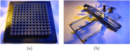
To improve the resolution, we built a second device for capturing ILFs consisting of a video camera with a f85° fisheye lens mounted to an x-y translation stage, shown in 6.26b. While this device could not acquire an ILF in a single moment, it did allow for capturing 1024 x 1024 pixel light probes at arbitrary density across the ILF plane Π. We used this device to capture several spatially varying lighting environments that included spotlight sources and sharp shadows at spatial resolutions of up to 32 x 32 light probe images.

We saw in Figure 6.6 the simple process of how a rendering algorithm traces rays into a light probe image to compute the light incident upon a particular point on a surface. Figure 6.27 shows the corresponding process for rendering a scene as illuminated by an ILF. As before, the ILF is mapped on to a geometric shape covering the scene, referred to as the auxiliary geometry, which can be a finite-distance dome or a more accurate geometric model of the environment. However, the renderer also keeps track of the original plane Π from which the ILF was captured. When an illumination ray sent from a point on a surface hits the auxilary geometry, the ray's line is intersected with the plane Π to determine the location and direction of that ray as captured by the ILF. In general, the ray will not strike the precise center of a light probe sample, so bilinear interpolation can be used to sample the ray's color and intensity from the ray's four closest light probe samples. Rays that do not correspond to rays observed within the field of view of the ILF can be extrapolated from the nearest observed rays of the same direction or assumed to be black.

Figure 6.28a shows a real scene consisting of four spheres and a 3D print of a sculpture model illuminated by spatially varying lighting. The scene was illuminated by two spotlights, one orange and one blue, with a card placed in front of the blue light to create a shadow across the scene. We photographed this scene under the lighting, and then removed the objects and positioned the ILF capture device shown in Figure 6.26b to capture the illumination incident to the plane of the table top. We then captured this illumination as a 30 x 30 array of light probe images spaced 1 inch apart in the x and y dimensions. The video camera was electronically controlled to capture each image at 16 different exposures one stop apart, ranging from 1 sec. to sec. To test the accuracy of the recovered lighting, we created a virtual version of the same scene and positioned a virtual camera to view the scene from the same viewpoint as the original camera. Then, we illuminated the virtual scene using the captured ILF to obtain the virtual rendering seen in Figure 6.28b. The virtual rendering shows the same spatially varying illumination properties on the objects, including the narrow orange spotlight and the half-shadowed blue light. Despite a slight misalignment between the virtual and real illumination, the rendering clearly shows the accuracy of using light captured on the plane of the table to extrapolate to areas above the table. For example, the base of the statue, where the ILF was captured, is in shadow from the blue light and fully illuminated by the orange light. Directly above, the head of the statue is illuminated by the blue light but does not fall within orange one. This effect is present in both the real photograph and the synthetic rendering.