11.3. Pictorial Tour
This section displays selected pictorial examples of some of the functions in OpenCV.
11.3.1. Functional groups
Manual section M1
This manual functional group contains static structures, image and array creation and handling, array and image arithmetic and logic, image and array statistics, and many dynamic structures. Trees are one structure, and as an example, a binarized image may be described in a tree form as a nested series of regions and holes as shown in Figure 11.2. Such trees may be used for letter recognition, for example.
Figure 11.2. M1: Contour tree. A binary image may described as a nested series of regions and holes. (Used with permission from [5, 6].)

Manual section M2
This functional group contains the basic image processing operations. For example, the Canny edge detector allows you to extract lines one pixel thick. The input is shown in Figure 11.3 and the output is shown in Figure 11.4.
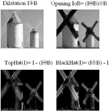
Morphological operators, used to clean up and isolate parts of images, are used quite a bit in machine and computer vision. The most basic operations are dilation (growing existing clumps of pixels) and erosion (eating away at existing clumps of pixels). To do this, you use a morphological kernel that has a control point and a spatial extent, as shown in Figure 11.5.
Figure 11.5. M2: Morphological kernel with control point and extent, and examples of how it grows (dilates) and shrinks (erodes) pixel groups in an image. (Used with permission from [5, 6].)
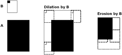
Figure 11.5 shows morphology in 2D. Morphology can also be used in higher dimensions such as considering image brightness or color values as a surface in 3D. Morphological erode and dilate can be combined in different ways, such as to close an object by dilation followed by erode or to open, which erodes and then dilates. Gradients and bump removal or isolation can also be done, as shown in Figures 11.6 and 11.7.
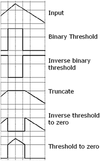
The types of thresholding operations that OpenCV supports are graphically portrayed in Figure 11.8.
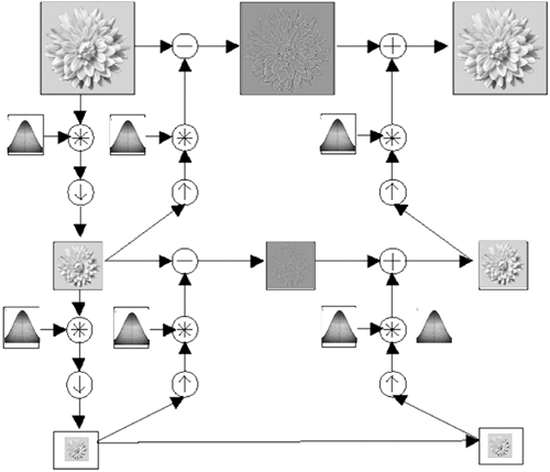
For computer vision, sensing at different resolutions is often necessary. OpenCV comes with an image pyramid or Laplacian pyramid function, as shown in Figure 11.9.
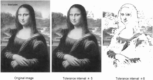
Floodfill is a graphics operator that is also used in computer vision for labeling regions as belonging together. OpenCV's floodfill can additionally fill upwards or downwards. Figure 11.10 shows an example of floodfilling.
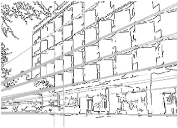
In addition to the Canny edge detector, you may want to find dominant straight lines in an image even if there might be discontinuities in those lines. The Hough transform is a robust method of finding dominant straight lines in an image. In Figure 11.11, we have the raw image of a building, and Figure 11.12 shows the dominant lines found by the Hough transform.
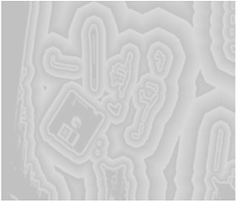
The final example we show from chapter M2 is Borgefors' distance transform [7]. The distance transform calculates the approximate distance from every binary image pixel to the nearest zero pixel. This is shown in Figures 11.13 and 11.14, where the raw image is thresholded and distance transformed.
Manual section M3
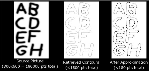
The contour processing functions can be used to turn binary images into contour representations for much faster processing. The contours may be simplified and shapes recognized by matching contour trees or by Maha-lanobis techniques. This is depicted in Figure 11.15 for a text recognition application.
Figure 11.15. M3: Contour recognition for OCR. Contours are found, simplified, and recognized. (Used with permission from [5, 6].)
Manual section M4
This section supports motion analysis and object tracking. The first thing supported is background segmentation. Using running averages for means and variances, the background may be learned in the presence of moving foreground and is shown in sequence in Figure 11.16.
Figure 11.16. M4: Learning the background in the presence of moving foreground and segmenting the two. (Used with permission from [5, 6].)

Once background-foreground segmentation has been accomplished in a frame, we can use the Motion History Image (MHI) functions to group and track motions. cvUpdateMotionHistory creates an MHI representation by overlaying foreground segmentations one over another with a floating-point value equal to the system timestamp in milliseconds. From there, gradients (cvCalcMotionGradient) of the MHI can be used to find the global motion (cvCalcGlobalOrientation), and floodfilling can segment out local motions (cvSegmentMotion). Contours of the most recent foreground image may be extracted and compared to templates to recognize poses (cvMatchShapes). Figure 11.17 shows from left to right a downward kick, raising arms, lowering arms, and recognizing a "T" pose. The smaller circles and lines are segmented motion of limbs, the larger circle and line is global motion.
Figure 11.17. M4: The smaller circles and lines are segmented motion of limbs, the larger circle and line is global motion. The final frame uses outer-contour-based shape recognition to recognize the pose. (Used with permission from [5, 6].)

The CamShift (continuously adapting mean shift) algorithm described in [11] uses a statistically robust probability mode tracker (mean shift) algorithm to track the mode of visual probability distributions, in this case flesh, as shown in Figure 11.18.
Figure 11.18. M4: CamShift, adaptive window-based tracking of the mode of a probability distribution, in this case, probability of flesh. (Used with permission from [5, 6].)

Snakes are a classic boundary tracking algorithm based on smoothed gradient energy minimization, seen in Figure 11.19.
Manual section M5
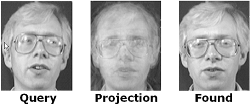
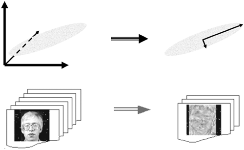
There are two recognition functions in this manual section: eigenobjects and embedded HMMs. For eigenobjects, if you think of an image as a point in a huge dimensional space (one dimension per pixel), then it seems reasonable that similar objects will tend to cluster together in this space. Eigenobjects take advantage of this by creating a lower dimensional space "basis" that captures most of the variance between these objects, as depicted in Figure 11.20, with a face image basis depicted at bottom. Once a basis has been learned, we can perform face recognition by projecting a new face into the face basis and selecting the nearest existing face as being the same person with confidence proportional to the distance (Mahalanobis distance) from the new face. Figure 11.21 shows a recognition example using this basis.
Figure 11.20. M5: Eigen idea explains most of the variance in a lower dimension.
Another object recognition technique is based on nested layers of HMMs [31]. Horizontal HMMs look for structure across the face and then feed their scores into an HMM that goes vertically down the face, as shown at left in Figure 11.22. This is called an embedded HMM (eHMM). At right in the figure is the default initialization for the eHMM to start its Viterbi training. Figure 11.23 shows the training and recognition process using eHMMs.
Figure 11.22. M5: Embedded HMM for recognition. On the left is the horizontal→vertical HMM layout; on the right is the default initialization for the HMM states. (Used with permission from [5, 6].)

Figure 11.23. M5: Training and recognition using an embedded HMM. (Used with permission from [5, 6].)

Manual section M6
Functions in this section are devoted to camera calibration, image rectification, and 3D tracking. We start with a function that helps track corners in a calibration checkerboard, cvFindChessBoardCornerGuesses, which is shown in operation in Figure 11.24.
When a sequence of calibration points has been tracked, cvCalibrate Camera_64d can be used to extract camera calibration parameters. These results can then be used to undistort a lens, as shown in Figure 11.25.
Figure 11.25. M6: Raw image at top, undistorted image at bottom after calibration. (Used with permission from [5, 6].)

After calibration, we can track a calibration checkerboard and use it to determine the 3D location of the checkerboard in each frame. This may be used for game control, as shown in Figure 11.26. OpenCV also includes support for tracking arbitrary, nonplanar objects using the POSIT (pose iteration) algorithm, which iterates between weak perspective (3D objects are 2D planes sitting at different depths) and strong perspective (objects are 3D) interpretation of points on objects. With mild constraints, POSIT rapidly converges to the true 3D object pose, which may also be used to track 3D objects.
Not shown here, but in the experimental manual section M7, are functions that further use calibrated cameras for stereo vision and 3D modeling. We next pictorially describe some of the demos that ship with OpenCV.
11.3.2. Demo tour
This section shows images of some of the demos that ship with OpenCV. Not shown is our version [28] of the Viola-Jones face tracker [40], and also not shown is the two-video camera stereo demo. Shown below are screen shots of the Calibration demo and the control screen for the multiple camera 3D tracking experimental demo in Figure 11.27. Also shown are color-based tracking using CamShift, Kalman filter, and condensation in Figure 11.28.
Figure 11.27. Demos: Automatic checkerboard tracking for camera calibration above and control screen for multiple-camera 3D below. (Used with permission from [5, 6].)

Figure 11.28. Demos: From top to bottom, CamShift tracking, Kalman filter, and condensation. (Used with permission from [5, 6].)

Figure 11.29 shows the HMM-based face recognition demo (also good for letter recognition), and finally, optical flow is shown in Figure 11.30.


