
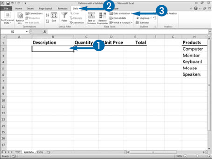
In Excel, you can restrict the values a user can enter into a cell. By restricting values, you help ensure that all worksheet entries are valid and that calculations based on them are valid as well. During data entry, a validation list forces anyone using your worksheet to select a value from a drop-down list rather than typing and potentially entering the wrong information. Validation lists save time and reduce errors.
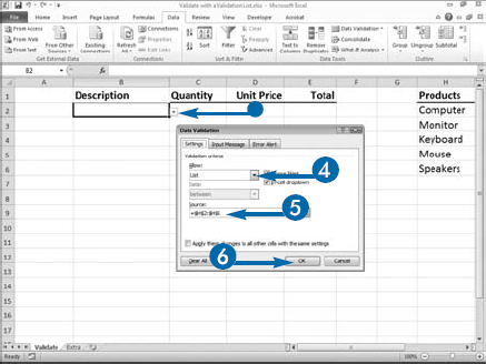
There are two methods that you can use to create a data validation list. First, if your list is short and does not change, you can type your list into the Source field of the Data Validation dialog box. For example, if your field collects gender, you can type "Male, Female" into the Source field. You must separate values with a comma. Second, if your list is long or if it changes, you can type the values into adjacent cells in a column or row. You may want to place the list in an out-of-the-way place on your worksheet or on a separate worksheet. With this method, if your list changes, just type the new values into the cells you have designated as the validation list. You can name the range. See Chapter 4 to learn how to name ranges. After you create your list of values, use the Source field in the Data Validation dialog box to assign the values to your validation list. You can click and drag to select the valid entries, or you can type = followed by the range, or type = followed by the range name.
After you have created a validation list, you can copy and paste it into other cells by using Paste Special's Validation option.
Validate with a Validation List
Create a Validation List


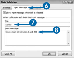
The Data Validation dialog box appears.


Alternatively, type the list of valid entries, with each entry followed by a comma.

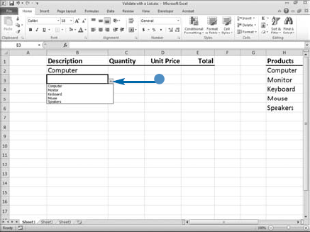
Excel creates a validation list in the cell you selected.
A menu appears.
The Paste Special dialog box appears.
Excel places the validation list in the cells you selected.
When you make an entry, you must pick from the list.

Extra
To remove a validation list, click in any cell that contains the validation list you want to remove, click the Home tab, and then click Find and Select in the Editing group. A menu appears. Click Go To Special. The Go To Special dialog box appears. Click Data Validation, click Same, and then click OK. The Go To Special dialog box closes. Click the Data tab and then click Data Validation in the Data Tools group. The Data Validation dialog box appears. Click the Settings tab. Click Clear All and then click OK.
If you base your validation list on a range of cells and any cell in that range is blank, and if you select the Ignore Blank check box (
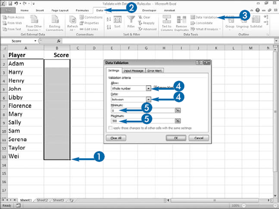
You can use data entry rules to ensure data is entered in the correct format, and you can restrict the data entered to whole numbers, decimals, dates, times, or a specific text length. You can also specify whether the values need to be between, not between, equal to, not equal to, greater than, less than, greater than or equal to, or less than or equal to the values you specify.
In addition, you can create an input message that appears when the user enters the cell and an error alert that displays if the user makes an incorrect entry. Error alerts can stop users, provide a warning, or just provide information. For example, when a user makes an incorrect entry, the Stop Error Alert style displays the error message you entered and the user cannot make an entry that does not meet your criteria. The Warning Alert style and the Information Alert style display a message but the user can still make an entry that does not meet your criteria. Input messages and error alerts consist of a title and a message.
After you create your data entry rule, you can copy and paste it into the appropriate cells by using the Paste Special Validation option. Refer to "Paste a Validation List" in the section "Validate with a Validation List" to learn how to copy and paste your data entry rule. If you click and drag to select the cells to which you want to apply your data validation rules and then open the Data Validation dialog box and create your data validation, Excel applies your validation to all the cells you selected.
Validate with Data Entry Rules
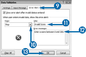
The Data Validation dialog box appears.


Choose Stop if you want to stop the entry of invalid data.
Choose Warning if you want to display a warning to the user, but not prevent the data entry.
Choose Information to provide information to the user.


Excel creates the data entry rule.
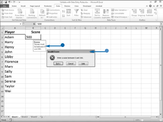
When a user clicks in the cell, Excel displays the input message.
When a user enters invalid data, Excel displays the error alert.
A comment is a bit of descriptive text that enables you to document your work. If someone else maintains your worksheet, or others use it in a workgroup, your comments can provide useful information. You can enter comments in any cell you want to document or otherwise annotate.
Comments in Excel do not appear until you choose to view them. Excel associates comments with individual cells and indicates their presence with a tiny red triangle in the cell's upper-right corner. View an individual comment by clicking in the cell or positioning your cursor over it. View all comments in a worksheet by clicking the Review tab and then clicking Show All Comments.
When you track your changes, Excel automatically generates a comment every time you copy or change a cell. The comment records what changed in the cell, who made the change, and the time and date of the change. To learn more about tracking changes, see the next section, "Track Changes."
When a comment gets in the way of another comment or blocks data, you can move it. Just position your cursor over the comment box border until the arrow turns into a four-sided arrow, click and drag the comment to a better location, and then release the mouse button. Your comment will remain in this position until you display all comments again.
When you sort, cut and paste, or copy and paste, comments move with the cell. Once you have created a comment, you can edit or delete it. You can also cycle through the comments in your worksheet by clicking Previous and Next on the Review tab.
Add Comments to Your Worksheet
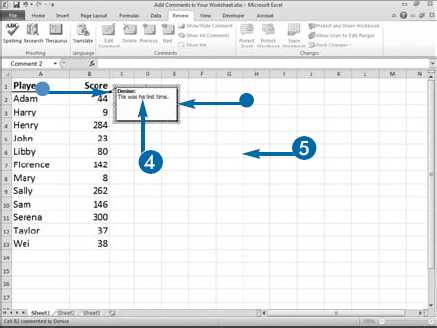
Add a Comment
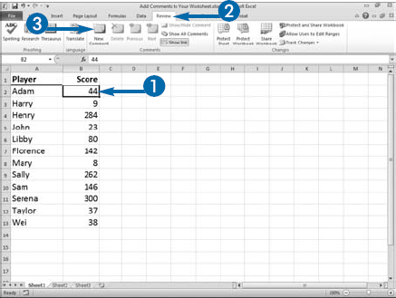
A comment box appears.
A red triangle appears.
Note: To apply bold or other formatting, select the text, right-click, click Format Comment, and then make changes as appropriate.
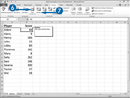
The comment box disappears.
Position the cursor over the cell to display your comment again.
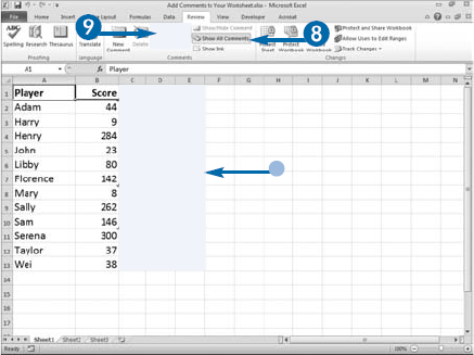
You can now see all the comments in the worksheet.
To close the comment boxes, click Show All Comments again.
Excel cycles through the comments.
By using change tracking, you can monitor the changes made to a shared workbook. A shared workbook is a workbook that can be edited by multiple people at the same time. When you turn on change tracking, your workbook automatically becomes a shared workbook. Change tracking keeps a log of changes. You can except or reject each change. This feature is especially useful when you have a workbook that needs to be reviewed by others. You can review each person's comments and changes and then finalize the workbook.
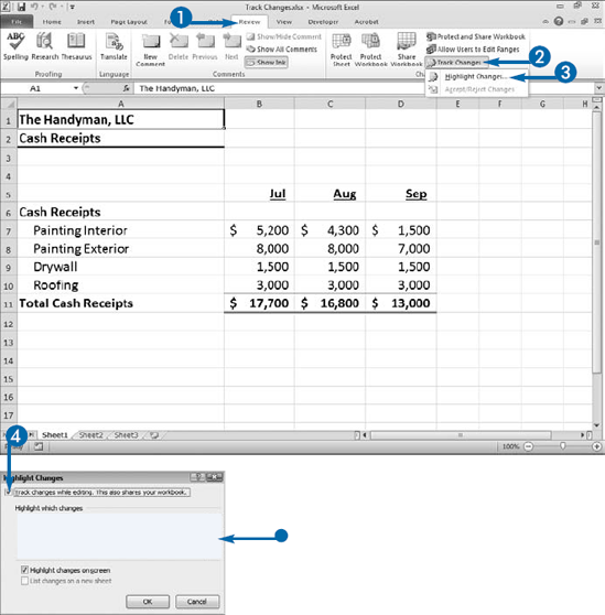
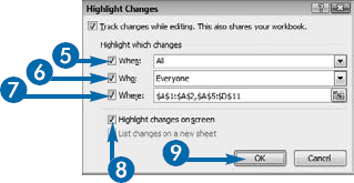
You can use the Highlight Changes dialog box to turn on change tracking. The Highlight changes dialog box has When, Who, and Where options. Use When to define the time after which edits are tracked — for example, after a specific date or since you last saved. Use Who to identify the group whose edits you want to track — for example, everyone in the workgroup, everyone but you, or a named individual. Use Where to specify the rows and columns you want to monitor.
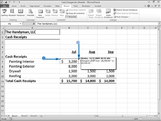
When someone makes a change, Excel indicates the change by placing a small purple triangle in the upper-left corner of the changed cell. Excel records cell changes in automatically generated cell comments. When Highlight Changes is activated, you can view these comments by moving your mouse pointer over the cells.
You can use the Accept or Reject Changes dialog box to review every change made to a worksheet and either accept or reject the change.
Before you share a workbook, enter and format your data because there are many features you cannot change in a shared workbook.
Track Changes
A menu appears.
The Highlight Changes dialog box appears.
The When, Who, and Where fields become available.
A message informs you that Excel will save your workbook.
Purple flags appear in edited cells.
To view a cell's comment, position your mouse cursor over the cell.
Note: For more about comments, see the previous section, "Add Comments to Your Worksheet."
Extra
When you share a workbook, you cannot modify the following: merged cells, conditional formats, data validations, charts, pictures, objects, hyperlinks, scenarios, outlines, subtotals, data tables, PivotTable reports, workbook and worksheet protection, and macros.
You can use the Accept or Reject Changes dialog box to review every change made to a worksheet and either accept or reject the change. To Access the Accept or Reject Changes dialog box, click the Review tab. Click Track Changes in the Changes group. A menu appears. Click Accept/Reject Changes. The Select Changes to Accept or Reject dialog box appears. Enter the criteria for the changes you want to review in the When, Who, and Where fields and then click OK. The Accept or Reject changes dialog box appears.
To view all worksheet changes after you or others make edits, open the Highlight Changes dialog box and click the List Changes on a New Sheet option (
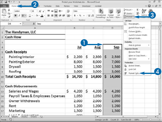
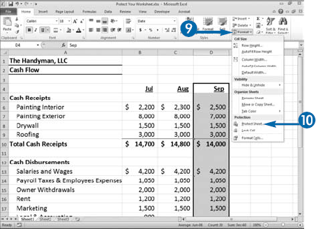
If you share your worksheets with others, you can lock them so others can view and print them but cannot make changes to the areas you do not allow them to change. Even if you do not share your worksheets, you may want to lock certain areas so you do not inadvertently make changes. Locking your worksheet enables you to allow users to make certain types of changes while disallowing others. You can choose which changes users can make. For example, you can allow users to make changes to formats; insert or delete columns, rows, or hyperlinks; sort; filter; use PivotTables; and/or edit objects or scenarios.
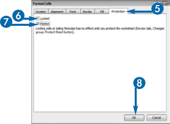
By default, when you lock a worksheet, Excel locks every cell in the worksheet and the formulas are visible to anyone who uses the worksheet. Prior to locking a worksheet, you can choose to leave specific cells unlocked and hide the formulas in specific cells. For example, you can lock every area except the current month. That way, users can make updates to the current month, but they cannot change previous months.
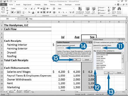
To protect your worksheet, you can enter a password in the Protect Sheet dialog box. If you add a password, only users who know the password can unlock the sheet. You should make your password strong by including upper- and lowercase letters, numbers, and symbols. Adding a password is optional. Keep a list of your worksheet passwords in a safe place, because you cannot recover a worksheet password. If you lose or forget your password, you can no longer access the locked areas of your worksheet.
Apply It
You can protect a workbook from unwanted changes. Click the Review tab, click Protect Workbook. The Protect Structure and Windows dialog box appears. Select Structure (
You can use the Allow Users to Edit Ranges dialog box to password-protect specific ranges in your worksheet. To password-protect a range, select the range you want to password-protect, click the Review tab, and then click Allow Users to Edit Ranges in the Changes group. The Allow Users to Edit Ranges dialog box appears. Click New. The New Range dialog box appears. In the Title field, name the range; in the Range password field, assign a password; then click OK. The Confirm Password dialog box appears. Retype your password, click OK, click Apply, and then click OK again. Your sheet must be protected and the range must be locked for this feature to work.
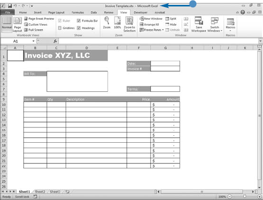
Templates are special-purpose workbooks you can use to create new worksheets. They can contain formats, styles, and specific content such as images, and column heads you want to reuse in other worksheets. Templates save you the work of re-creating workbooks for recurring purposes such as filling out invoices and preparing monthly reports.
You create a template by designing a generic workbook that contains the worksheet layouts you want. You can create custom styles, number formats, macros, and formulas and include them in your template. For example, if you regularly use Excel to create and issue invoices, you can create an automatically calculating invoice that includes your logo and other basic information.
Your custom template includes all the changes you have made to your workbook, including formats, formulas, and such changes as opening multiple windows or deleting tabs. Saving formulas with your template causes your worksheet to calculate automatically. Saving formats saves you from having to re-create them.
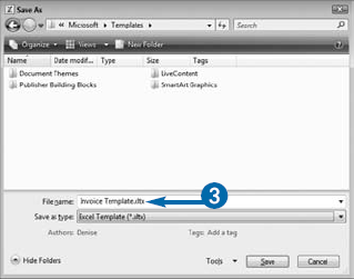
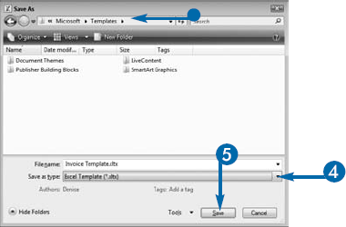
When you work with a template, you edit a copy — not the original — so you retain the original template to use when structuring other workbooks. Excel 2010 workbooks ordinarily have an .xlsx file extension. Saving an Excel workbook as a template creates a file with an .xltx extension.
Excel comes with ready-made templates that serve basic business purposes such as invoicing. You can use the Available Templates dialog box to access these templates. To access the Available Templates dialog box, click the File tab and then click New. You can also use the Available Templates dialog box to access Office.com, which has several categories of templates that you can download.

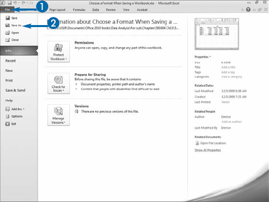
After you create a worksheet, you may want to share it with others. The file format you choose when you save your file is important. The default format for Office 2010 is Excel Workbook (*.xlsx). This file format was introduced in Office 2007. The smaller files it creates are easily accessible in other software programs because they are in Extensible Markup Language (XML) format, which is a data-exchange standard.
Versions prior to Excel 2007 did not use XML as the default format. These files have an.xls extension. If you want to share your documents with people who use Excel 97–2003, you can save your file as an Excel 97–2003 workbook (*.xls). Features that are not supported in earlier versions of Excel are lost when you save your file as an Excel 97–2003 workbook.
If you have a computer with Excel 97–2003 installed, you can go to the Office Update Web site and download the Microsoft Office Compatibility Pack for Excel. After you install the Compatibility Pack, you can open Excel Workbook *.xlsx files in Excel 97–2003. Excel Workbook *.xlsx formatting and other features may not display in the earlier version, but they are still available when you open the file again in Excel 2010.
If you want to see the XML layout for an Excel 2010 file, change the file extension on the file to .zip and then double-click the file. The file opens and several folders and files appear. Double-click the files to open and view them.
You can also save your worksheet in other file formats, including Web Page formats (*.htm; *.html) and several text-based formats, such as Text (MS-DOS) (*.txt), Text (Macintosh) (*.txt), and CSV (comma-delimited). These formats save the worksheet as text, which can be read by other applications, or in Hypertext Markup Language (HTML), which can be read by browsers.

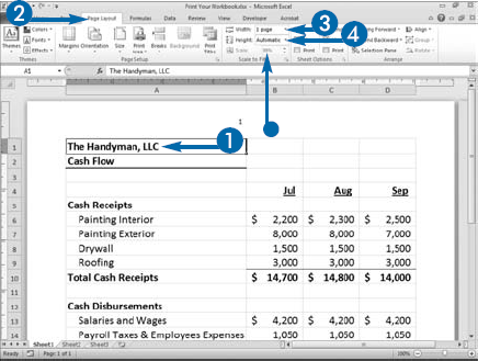
The most common way to share a workbook with others is to print the worksheets and distribute paper copies. Excel has several features to help you format and print your worksheets. You can select the worksheet's margin size, orientation, paper size, print area, page breaks, and much more. If you want to see a live view of how print settings affect your report, use Page Layout view.
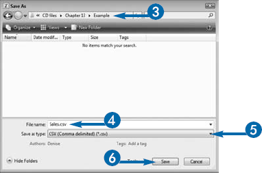
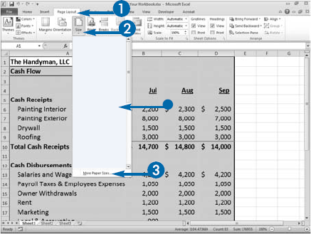
You can print part of your worksheet or your entire worksheet. If you want to print part of your worksheet, you can use the Set Print Area option on the Page Layout tab to tell Excel the area you want to print.
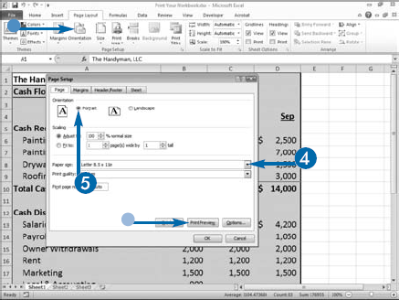
On the Page Layout tab, use the Size option to tell Excel the size of your paper. When you click Size, the most commonly used paper sizes appear on the menu. If you do not see the paper size you are using, click More Paper Sizes and select a size from the Page tab of the Page Setup dialog box. While in the Page Setup dialog box, you can select the orientation of your worksheet: Landscape or Portrait. Selecting Portrait makes the shortest edges of your paper the top and bottom and the longest edges of your paper the sides. Selecting Landscape makes the longest edges of your paper the top and bottom and the shortest edges of your paper the sides.
If at any time during the process of setting up your document for printing, you want to see a preview of how your printed document will look, you can click the Print Preview button, which is located on every tab in the Page Setup dialog box.
Print Your Workbook
Set the Print Area
A menu appears.
Excel sets the print area.
Set the Orientation and Page Size
Alternatively, click the Page Orientation button and select an orientation.
Click Print Preview to see a preview of your document.
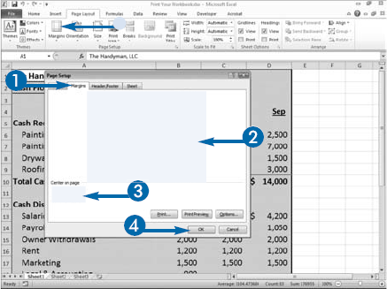
Set the Margins
Alternatively, click the Margins button and then set the margins.
The Page Setup dialog box closes.
Excel sets the margins.
Extra
Clicking the launcher in the Page Setup, Scale to Fit, or Sheet Options group on the Page Layout tab opens the Page Setup dialog box. Every page of the Page Setup Dialog box has a Print Preview button. If you want to see a preview of how your document will look when you print it, click the Print Preview button. You can use the buttons below your document to scroll through your document. If you want to view the margins, select the Show Margins button (
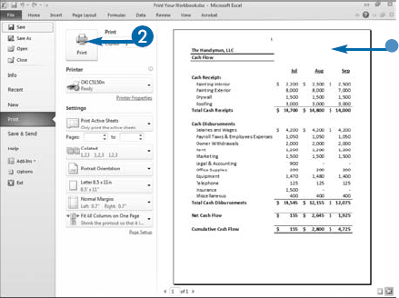
Click Page Setup, which is located under the print options, to open the Page Setup dialog box. Use the Page Setup dialog box to adjust your settings. When you are ready to print, click the Print button.
On the Ribbon, you can click Breaks in the Page Setup group of the Page Layout tab to specify where a new page is to begin in your printed copy. Select where you want to place the break. Click the Breaks button and then click Insert Page Break. Excel inserts a page break above and to the left of your selection.
Margins define the amount of white space that surrounds your document. You can apply Excel's predefined margins by selecting them from the Margins menu, or you can open the Page Setup dialog box to define your margins. By default, Excel places your data in the upper-right corner of the page. The Margins tab in the Page Setup dialog box has options you can use to center your worksheet horizontally and/or vertically.
A header is text that prints across the top of every page of your worksheet. A footer is text that prints across the bottom of every page of your worksheet. You can set the amount of margin space Excel reserves for headers and footers on the Margins tab.
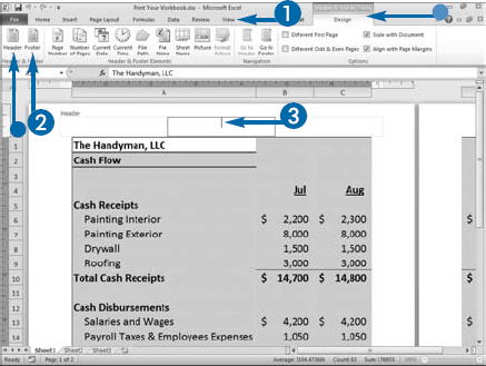
When you click in the header or footer area while in Page Layout view, the Header and Footer tools become available. You can use the Design tab to tell Excel what data you want to include in your header and/or footer. The Header and Footer options provide you with a list of predefined headers and footers. In the Header & Footer Elements group, you can select the options you want to place in your header or footer.
If your data does not fit on the number of pages you want, you can scale your data. You can use a percentage to make your data larger or smaller. For example, setting the scale to 110 makes your data 10 percent larger than its normal size. Setting the scale to 90 makes your data 90 percent of its normal size. You can also scale your data by selecting the number of pages on which you want your data to fit. If you choose Automatic, Excel determines the amount of data to put on each page.
Create a Header or Footer
Excel changes to layout view.
Click Normal to return to normal view.
The left area places information on the left.
The center area places information in the center.
The right area places information on the right.
The Header & Footer tools become available.
Excel places the option in the area you selected.
This example adds a page number in the center.
Click Header or Footer to use a predefined header or footer.

Excel scales your document.
Alternatively, click select a scale option to scale your document.
The Print dialog box appears.
The Print Preview.
Excel prints your worksheet.
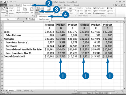
You can print noncontiguous areas of your worksheet, thereby limiting your printing to the information that is of relevance. This feature involves little more than selecting the cells you want to print.
There are many reasons why you may want to print noncontiguous areas of your worksheet. For example, if you have sales data for several products, each in a column, you can select and print only the columns in which you are interested. You select noncontiguous areas of the worksheet by pressing and holding Ctrl as you click and drag. After you select areas, you set them as the print area. Print areas stay in effect until you clear them. You can add to the print area by selecting a range, clicking Page Layout, and then clicking Print Area; or by clicking Page Layout and then clicking Add to Print Area. To clear the print area, click Page Layout, click Print Area, and then click Clear Print Area.
Excel places the ranges you select in the Print Area field in the Page Setup dialog box. A comma follows each range. Use the same format if you want to enter your print ranges manually into the Print Area field.
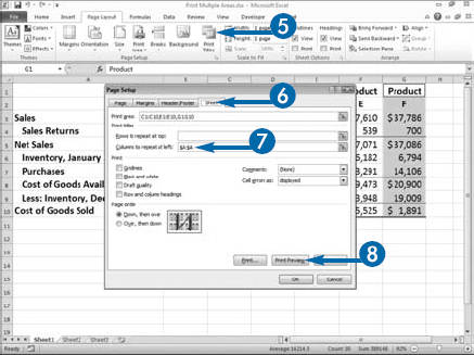
When printing a worksheet, you may have column headings or row labels you want to print with each selection. You can specify the rows you want to repeat at the top or the columns you want to repeat down the left side of every page you print by entering the ranges in the Rows to Repeat at Top and Columns to Repeat at Left fields in the Page Setup dialog box.
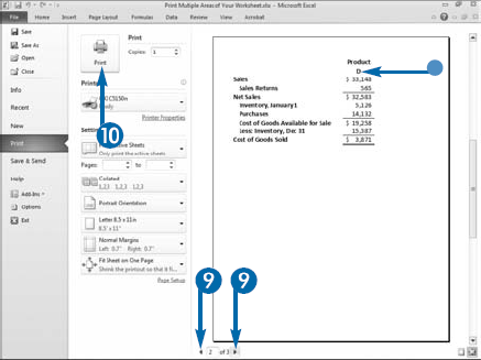
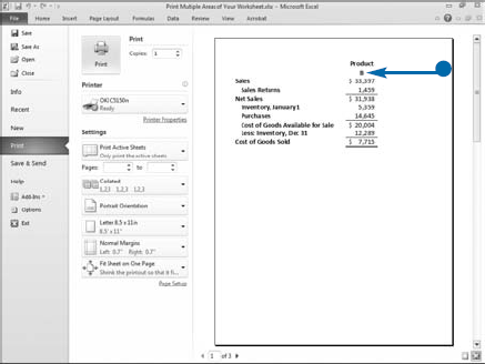
When you print a worksheet with multiple selected areas, each area prints on its own page.
Print Multiple Areas of Your Worksheet
Excel sets the print area.
The Page Setup dialog box appears.
The Print Preview window shows the next page of the printout, which contains" an area you selected in Step 1.
Excel prints the selected areas.
Extra
To open the Page Setup dialog box, click the launcher in the Page Setup group. You can use the Header/Footer tab in the Page Setup dialog box to add page numbers as well as a header or footer. Click Custom Header or Custom Footer to add dates and page numbers to each page.
You can access print options such as number of copies to print, printer to use, sheets and area to print by clicking the File tab and then clicking Print on the menu that appears.
You can print row numbers and column letters on every page. Click the launcher in the Page Setup group on the Page Layout tab to open the Page Setup dialog box. On the Sheet tab, click Row and column headings (