
7.7 Confidence Intervals
Let us return to our research team that wants to investigate how a certain diet affects the blood pressure of healthy people. Since they cannot test the diet on the whole population of healthy people they have chosen a representative sample consisting of 15 persons, which is a common sample size for these types of investigations. Before the tests they measure the blood pressures of their test persons. After 15 days of diet they measure the blood pressures again. Calculating the difference between the systolic blood pressure after and before the diet for each test person, they obtain the following results (in mm Hg):
![]()
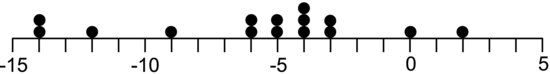
There seems to be a large variation in the results. Two persons’ blood pressures drop by as much as 14 mm Hg, but in one person there is actually an increase. What can we say about the effect of the diet based on these figures? As a first step it is always useful to display the data graphically in a diagram. Figure 7.14 shows that the drop after the diet is about 4 mm Hg for most persons. A few persons show larger drops than this, while others show no effect or even an increase. The mean difference in the sample is −5.8 mm Hg. But this is a limited sample. The interesting question is what the mean difference in blood pressure would have been in the whole population. Is it possible to be, say, 95% certain that the diet is effective?
Figure 7.14 Differences in blood pressure before and after diet.
Stating our problem in general terms, we have a sample from an unknown population and want to estimate a population parameter at a certain level of confidence. The interesting parameter in our case is the mean difference in blood pressure resulting from the diet and we want to have 95% confidence in our estimate of this parameter. Recall from the central limit theorem that, for large sample sizes n, the mean ![]() of a sample approximately follows a normal distribution with mean μ and standard deviation
of a sample approximately follows a normal distribution with mean μ and standard deviation ![]() . Using Equation 7.10 we may thereby make the variable transformation:
. Using Equation 7.10 we may thereby make the variable transformation:
Figure 7.15 There is 95% probability of finding Z in the white region. There is thus 5% probability of finding Z in the shaded regions. This probability is called α. Since each shaded region corresponds to α/2, the critical values limiting the 95% interval are called Zα/2.
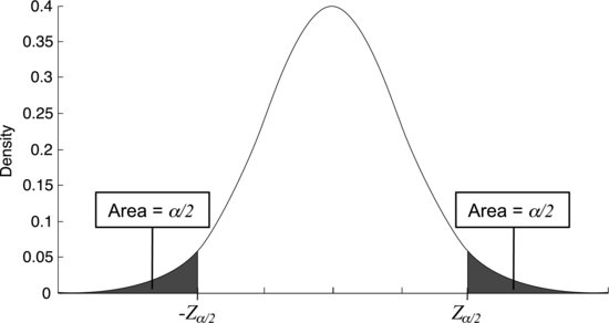
and obtain a variable that follows the standard normal distribution. Since this distribution is known it is now easy to find an interval such that there is 95% probability of finding Z within it.
Alternatively, we could say that there should be 5% probability of finding Z outside the interval; this probability is commonly written α. Looking at Figure 7.15 we see that α corresponds to the shaded areas under the tails of the curve. Each of the two areas corresponds to 2.5% probability, or α/2. The critical values of Z that limit the interval are, therefore, called ![]() and
and ![]() . They may be found in the table of standard normal probabilities in the Appendix. Looking there you will find that a 2.5% probability corresponds to
. They may be found in the table of standard normal probabilities in the Appendix. Looking there you will find that a 2.5% probability corresponds to ![]() = 1.96.
= 1.96.
Box 7.2 shows the steps involved in determining the 95% confidence interval for the population mean μ. The first step states that, by definition, there is 95% probability of finding Z between ![]() and
and ![]() . In the next step we replace Z using Equation 7.11, to get an expression that contains the population mean μ. Finally, we rearrange the terms to obtain an interval for μ. We arrive at the following expression for the 95% confidence interval for μ:
. In the next step we replace Z using Equation 7.11, to get an expression that contains the population mean μ. Finally, we rearrange the terms to obtain an interval for μ. We arrive at the following expression for the 95% confidence interval for μ:
The meaning of this is that, if we take repeated samples and calculate the confidence intervals from them, we expect these intervals to include μ 95% of the time.
We are almost finished solving the problem, but there are two problems with Equation 7.12. Firstly, since we are sampling from an unknown distribution, we do not know σ. Secondly, the central limit theorem requires a large sample, and our sample of 15 people is relatively small. These problems can be remedied by using another distribution that is more suited for small samples, called the t-distribution.