
Theoretical and Numerical Perspectives and Field Observations for the Design and Performance Evaluation of Embankments Constructed on Soft Marine Clay
Buddhima Indraratna1; I. Sathananthan2; C. Bamunawita2; A.S. Balasubramaniam3 1 Professor and Research Director, Centre for Geomechanics and Railway Engineering, Faculty of Engineering and Information Sciences, University of Wollongong, NSW, Australia
2 Former Student, Centre for Geomechanics and Railway Engineering, University of Wollongong, Australia
3 Professor, School of Engineering, Griffith University, Gold Coast, Australia
Abstract
In this chapter, a two-dimensional plane strain solution is adopted for the embankment analysis, which includes the effects of a smear zone caused by mandrel driven vertical drains. The equivalent (transformed) permeability coefficients are incorporated in finite element codes, employing modified Cam-clay theory. Selected numerical studies have been carried out to study the effect of embankment slope, construction rate, and drain spacing on the failure of the soft clay foundation. Finally, the observed and predicted performances of well-instrumented full-scale trial embankments built on soft Malaysian marine clay have been discussed in detail. The predicted results agree with the field measurements.
Acknowledgments
The authors acknowledge the Malaysian Highway Authority for providing the trial embankments data. Significant extracts and adaptations of technical content of this chapter have come from the authors’ previous publications such as the ASCE and Canadian Geotechnical Journal papers, as cited in the text and listed in the references section.
3.1 Introduction
Rapid development and associated urbanization have compelled engineers to construct earth structures, including major highways, over soft clay deposits of low-bearing capacity coupled with excessive settlement characteristics. In the coastal regions of Australia and Southeast Asia, soft clays are widespread, particularly in the vicinity of capital cities. Because soft soils are weak, unreinforced embankments can only be built 4–5 m high. However, higher embankments are often needed and their rapid construction is pertinent given the usual stringent deadlines. To achieve these goals, special construction measures such as lightweight embankment fill, the provision of reinforcement at the bottom of the embankment, and suitable ground improvement techniques and staged embankment construction must be considered. The application of prefabricated vertical drains (PVDs) with preloading (vacuum pressure or surcharge) has become common practice and is one of the most effective techniques for ground improvement.
Many improvement techniques have been developed to suit certain soil conditions, with most soft clay methods based on consolidation. Preloading with vertical drains is a successful ground improvement technique, which involves the loading of the ground surface to induce most of the ultimate settlement of the underlying soft formation. Usually, a surcharge load equal to or greater than the expected foundation loading is applied to accelerate consolidation with the aid of vertical drains. The application of vacuum pressure can reduce the amount of surcharge fill material required to obtain the same consolidation settlement because it generates suction, which increases the effective stress and accelerates consolidation.
Consolidation of soil is the process of decreasing the volume in saturated soils by expelling the pore water. Therefore, the consolidation rate is governed by the compressibility, permeability, and length of the drainage path. The settlement level is directly related to the void ratio change, which is directly proportional to the rate of dissipation of excess pore water pressure. For three decades, vertical drains with preloading have been used to accelerate the consolidation process before construction commences.
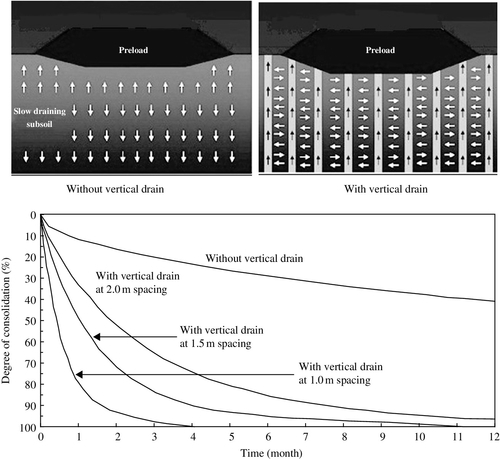
Preloading on its own can reduce the total and differential settlement facilitating the choice of foundations, but when vertical drains are used with preloading the settlement process can be accelerated considerably (Fig. 3.1). The main advantages of vertical drains are: (1) to increase the shear strength of soil through a decreased void ratio and moisture content, (2) to decrease the time for preloading to minimize the same level of postconstruction settlement, (3) to reduce differential settlement during primary consolidation, and (4) to curtail the height of surcharge fill required to achieve desired precompression.
3.2 Installation and monitoring of vertical drains
Before installing a vertical drain it is essential to prepare the site. This may involve removing surface vegetation and debris and grading the site for a sand blanket to act as a medium for expelling water from the drains and an appropriate working mat. Vertical drains can be installed by the washing jet method, the static method, or the dynamic method. The washing jet method is primarily used when installing large diameter sand drains, whereby sand is washed in through the jet pipe. PVDs are usually installed by the static or dynamic method (Fig. 3.2). In the latter, the mandrel is driven into the ground with either a vibrating or drop hammer, but in the former, the mandrel is pushed into the soil by a static load. The static method usually causes less ground disturbances and is preferred for more sensitive soils. Although faster, the dynamic methods generate higher excess pore pressures and a greater disturbance of the soil around the mandrel during installation.

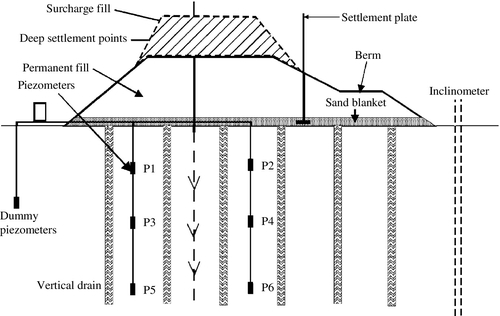
On major projects, instrumentation is essential for verifying performance and observing design amendments, as warranted, to prevent unacceptable displacement. Figure 3.3 shows a typical scheme of instruments required to monitor the performance of a soft clay foundation beneath an embankment containing PVDs. The most commonly used instruments are inclinometers, settlement indicators, and piezometers, as described in the following subsections.
3.2.1 Inclinometers
Inclinometers are used to monitor the lateral (transverse) movements of natural slopes or embankments. An inclinometer casing has a grooved metal or plastic pipe that is placed into a borehole (Dunnicliff, 1988). The space between the wall of the borehole and the casing is backfilled with a sand or gravel grout. The bottom of the pipe must rest on a firm base to achieve a stable point of fixity. To monitor embankment performance, inclinometers are normally placed at or near the toe of the embankment where excessive lateral movement is usually of some concern.
3.2.2 Settlement indicators
Settlement plates or points are commonly installed where significant settlement is predicted (Dunnicliff, 1988) to record the magnitude and rate of settlement under a load. Therefore, they should be placed immediately after installing the vertical drains. In the simplest form, this instrument is a settlement plate consisting of a steel plate placed on the ground before construction of the embankment. Surface settlement points measure vertical displacement with depth, for example, along an embankment centerline. Typically, a reference rod and protecting pipe are attached to the settlement-monitoring platform. Settlement is often evaluated periodically until the surcharge embankment is completed, then at a reduced frequency, measuring the elevation of the top of the reference rod. Benchmarks used for reference data must be stable and remote from all other possible vertical movements. Further information about settlement points is given elsewhere (Dunnicliff, 1988).
3.2.3 Piezometers
A detailed description and analysis of various types of piezometers to measure in situ pore water pressure are presented by Hanna (1985) and Dunnicliff (1988). Piezometers should be installed at the bottom of the sand blanket, at various intermediate depths within the compressible layer. A dummy piezometer is usually installed a sufficient distance away from the embankment to record natural groundwater level, and excess pore water pressure at a given location is determined by comparison with the “dummy” level.
3.3 Drain properties
3.3.1 Diameter of influence zone
As shown in Fig. 3.4, the equivalent diameter of the influence zone (De) can be found in terms of the drain spacing (S) as follows (Hansbo, 1981):
and
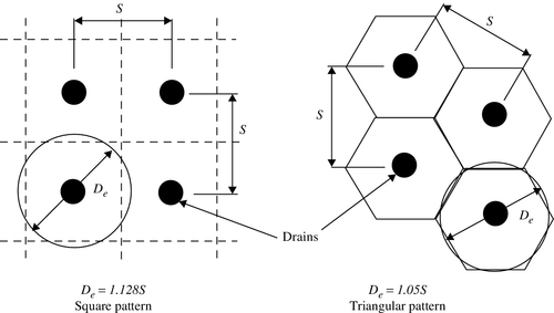
Drains in a square pattern may be easier to lay out and control during installation in the field but a triangular pattern usually provides a more uniform consolidation between them.
3.3.2 Equivalent drain diameter of band-shaped vertical drain
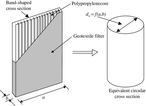
Most prefabricated drains have a rectangular cross section (band-shaped, Fig. 3.5), but for design purposes, the rectangular (width a, thickness b) section has to be converted into an equivalent circle with a diameter of dw, because the conventional theory of radial consolidation assumes that drains are circular.
The following typical equation is used to determine the equivalent drain diameter:
Atkinson and Eldred (1981) proposed that a reduction factor of π/4 should be applied to Eq. (3.3) to take account of the corner effect, where the flow lines rapidly converge. From the finite element studies, Rixner et al. (1986) proposed that
Pradhan et al. (1993) suggested that the equivalent diameter of band-shaped drains should be estimated by considering the flow net around the soil cylinder of diameter de (Fig. 3.6). The mean-square distance of their flow net is calculated as

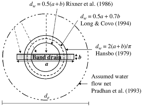
More recently, Long and Covo (1994) found that the equivalent diameter dw could be computed using an electrical analog field plotter:
3.3.3 Discharge capacity
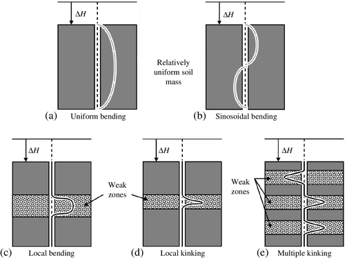
The discharge capacity is probably the most important parameter that controls the performance of prefabricated vertical drains. According to Holtz et al. (1991), the discharge capacity depends primarily on the following factors (Fig. 3.7): (1) the area of the drain core available for flow, (2) the effect of lateral earth pressure, (3) possible folding, bending, and crimping of the drain, and (4) infiltration of fine particles into the drain filter.
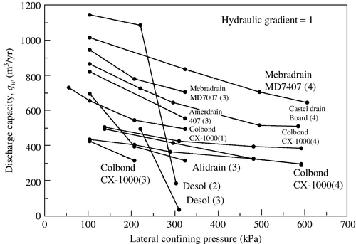
The current recommended values are given in Table 3.1 and the discharge capacities of various types of drains are shown in Fig. 3.8 as a function of lateral confining pressure.
Table 3.1
Current recommended values for specification of discharge capacity
| Source | Value | Lateral stress (kPa) |
| Kremer et al. (1982) | 256 | 100 |
| Kremer et al. (1983) | 790 | 15 |
| Jamiolkowski et al. (1983) | 10–15 | 300–500 |
| Rixner et al. (1986) | 100 | Not given |
| Hansbo (1987) | 50–100 | Not given |
| Holtz et al. (1989) | 100–150 | 300–500 |
| de Jager and Oostveen (1990) | 315–1580 | 150–300 |
3.4 Factors influencing the vertical drain efficiency
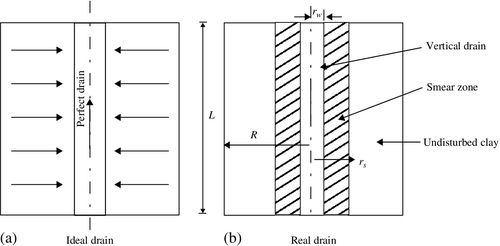
3.4.1 Smear zone
In the field, vertical drains are installed using a steel mandrel, which is pushed into ground statically or dynamically then withdrawn, leaving the drain in the subsoil. This process causes significant remolding of the subsoil, especially in the immediate vicinity of the mandrel. The resulting smear zone will have reduced lateral permeability, which adversely affects consolidation process.
The combined effect of permeability and compressibility within the smear zone causes a different behavior from the undisturbed soil. Predicting soil behavior surrounding the drain requires an accurate estimation of the smear zone properties. In many classical solutions (Barron, 1948; Hansbo, 1981; Indraratna et al., 1997), the influence of the smear zone is considered with an idealized two-zone model.
Two parameters are necessary to characterize the smear effect, namely, the diameter of the smear zone (ds) and the permeability ratio (kh/ks), that is, the value in the undisturbed zone (kh) over the smear zone (ks). Both the diameter of the smear zone and its permeability are difficult to quantify and determine from laboratory tests, and, so far, there is no comprehensive or standard method of measuring them. The extent of the smear zone and its permeability vary with the installation procedure, size, and shape of the mandrel, and the type and sensitivity of soil (macro fabric). Field and laboratory observations (Indraratna and Redana, 1998) indicated a continuous variation of soil permeability with the radial distance away from the drain centerline. Also, the smear zone diameter (ds) has been the subject of much discussion in literature dealing with PVD.
Investigations by Holtz and Holm (1973) and Akagi (1977) indicate that
where dm is the diameter of the circle with an area equal to the cross-sectional area of the mandrel. Jamiolkowski and Lancellotta (1981) proposed that
Hansbo (1981, 1997) proposed a different relationship:
Based on laboratory study and back-analysis, Bergado et al. (1991) proposed that the following relation could be assumed:
Indraratna and Redana (1998) proposed that the estimated smear zone could be as large as (4 − 5)dw. This proposed relationship was verified using a specially designed large-scale consolidometer (Indraratna and Redana, 1995). Figure 3.9 shows the variation of the kh/kv ratio along the radial distance from the central drain. According to Hansbo (1987) and Bergado et al. (1991), the kh/kv ratio was found to be close to unity in the smear zone. This agrees with the study by Indraratna and Redana (1998). More recently, the primary author and his coworkers at the University of Wollongong attempted to estimate the extent of the smear zone caused by mandrel installation using the cylindrical cavity expansion theory. They used the modified Cam-clay (MCC) model and verified that the extent of the smear zone proposed by Indraratna and Redana (1998) was reasonable. Most recent results indicate that for most soft clays the extent of the smear zone is between 4dw and 6dw. The recommended smear zone parameters by different researchers are listed in Table 3.2.
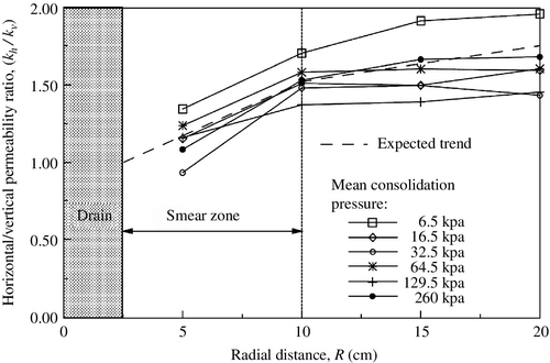
Table 3.2
Proposed smear zone parameters
| Source | Extent | Permeability | Remarks |
| Barron (1948) | rs = 1.6rm | kh/ks = 3 | Assumed |
| Hansbo (1979) | rs = 1.5 ~ 3rm | Open | Based on available literature at that time |
| Hansbo (1981) | rs = 1.5rm | kh/ks = 3 | Assumed in case study |
| Bergado et al. (1991) | rs = 2rm | kh/kv = 1 | Laboratory investigation and back-analysis for soft Bangkok clay |
| Onoue et al. (1991) | rs = 1.6rm | kh/ks = 3 | From test interpretation |
| Almeida and Ferreira (1993) | rs = 1.5 ~ 2rm | kh/ks = 3 ~ 6 | Based on experience |
| Indraratna and Redana (1998) | rs = 4 ~ 5rm | kh/kv = 1.15 | Laboratory investigation (for Sydney clay) |
| Chai and Miura (1999) | rs = 2 ~ 3rm | kh/ks = Cf(kh/ks) | Cf the ratio between lab and field values |
| Hird and Moseley (2000) | rs = 1.6rm | kh/ks = 3 | Recommend for design |
| Xiao (2000) | rs = 4rm | kh/ks = 1.3 | Laboratory investigation (for Kaolin clay) |
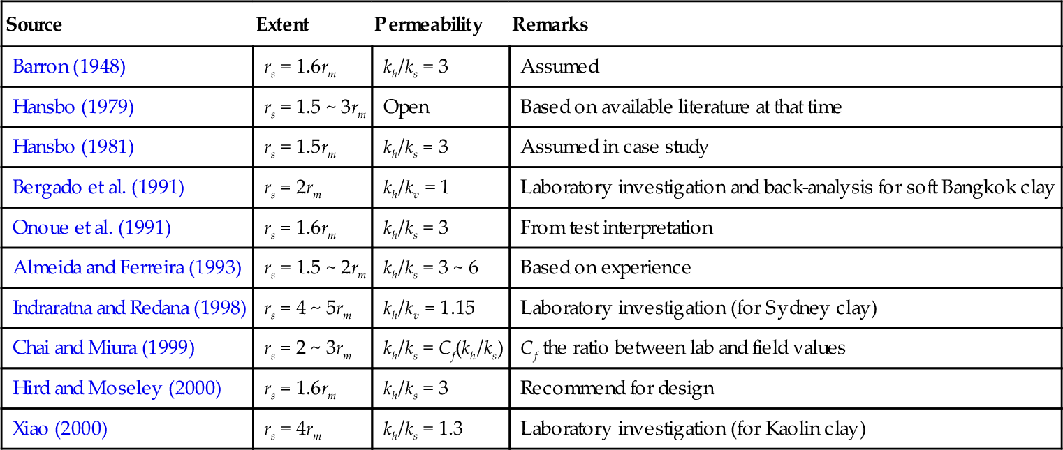
rs = radius of smear zone.
3.4.2 Effect of a sand mat
Part or all water ingress to drains will flow to the ground first and then drain out through the sand mat. Because the hydraulic conductivity of sand is considerably higher than clay, it can usually be assumed that there is no hydraulic resistance in the sand mat. However, in some cases, depending on local materials, lower quality clayey sand may be used as a sand mat. In these instances, the hydraulic resistance in the sand mat may influence the rate of consolidation of the clay subsoil, the amount of which is a function of the hydraulic conductivity of the sand as well as the embankment geometry.
3.4.3 Well resistance
Well resistance refers to the finite permeability of the vertical drain with respect to the soil. Head loss occurs when water flows along the drain and delays radial consolidation. Well resistance is controlled not only by the discharge capacity of the drain qw, but also by the permeability of the soil kh, the maximum discharge length lm, and any geometric deficiencies (bending, kinks, etc.) on the drains.
Mesri and Lo (1991) proposed the governing equation for vertical flow within the vertical drain in terms of excess pore water pressure at soil–drain interface. Based on Mesri’s equation, a well-resistance factor (R) is defined as
Analysis of the field performance of vertical drains indicated that the well resistance is negligible when R > 5. In other words, the minimum discharge capacity qw(min) of vertical drains required for negligible well resistance may be determined from
This relationship is illustrated in Fig. 3.10 for most typical values of kh and lm.
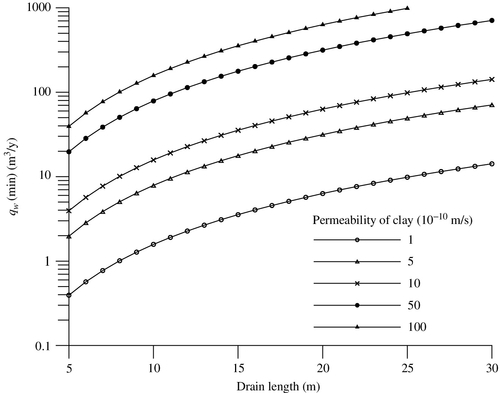
Table 3.3 summarizes the well-resistance indices proposed by various investigators to evaluate the influence of finite discharge capacity of vertical drains. Note that the proposed indices are also transformed to the well-resistance factor (R) proposed by Mesri and Lo (1991). These indices depend on R, except for in the expression proposed by Aboshi and Yoshikuni (1967) and Stamatopoulos and Kotzias (1985), in which the drain spacing is also included.
Table 3.3
Summary of proposed well-resistance indices
| Source | Index of well resistance |
| Aboshi and Yoshikuni (1967) |  |
| Yoshikuni and Nakanodo (1974), Onoue (1988) |  |
| Hansbo (1981) |  |
| Stamatopoulos and Kotzias (1985) |  |
| Zeng and Xie (1989) |  |
| Mesri and Lo (1991) |  |
n = De/dw is the spacing ratio.
In general, laboratory and field data indicate that the discharge capacities of most commercial PVDs have little influence on the consolidation rate of clay, especially for drains that are not too long (Indraratna et al., 1994). For values of qw > 100–150 m3/year (in the field) and where drains are shorter than 30 m, there should be no significant increase in the consolidation time. Given these circumstances, it may be claimed that for commercial PVDs, well resistance is usually negligible in most practical situations unless the drains are excessively long and geometric deficiencies occur during installation (bending, kinks, etc.). In most soft clays, well resistance can be ignored for PVD < 15 m long.
3.5 Development of vertical drain theory
Analytical solutions already developed for consolidation of ground improved with vertical drains invariably employ the “unit cell” model, as illustrated in Fig. 3.11. The theory for radial drainage consolidation has been addressed by many researchers (Rendulic, 1936; Carillo, 1942; Barron, 1948; Yoshikuni and Nakanodo, 1974; Hansbo, 1981; Onoue, 1988; Zeng and Xie, 1989).
3.5.1 Rendulic and Carillo diffusion theory
Rendulic (1936) formulated and solved the differential equation for one-dimensional vertical compression by radial flows
where r is the coordinate and ch the horizontal coefficient of consolidation (kh/γwmv).
Carillo (1942) showed that for radial drainage and associated 1D consolidation, the excess pore water pressure ur,z is given by
where, ur and uz are the excess pore water pressure due to radial flow and vertical flow only, and u0 is the initial pore water pressure. By substituting the average excess pore water pressure into Eq. (3.16), the average degree of consolidation of the compressible stratum can be obtained by combining Uz and Ur, thus
where Ū is the average degree of consolidation of the clay at time t for combined vertical and radial flow, and Ūz and Ūr are the average degree of consolidation at time t for vertical and radial flow, respectively. It should be noted that both Rendulic and Carillo’s solutions are for “ideal” drains only (infinite discharge capacity with no smear zone).
3.5.2 Barron—equal strain rigorous solution
Barron (1948) addressed the smear and well-resistance effects that can decrease the performance of vertical drains. He presented closed-form solutions for two extreme cases for radial drainage-induced consolidation, namely, free strain and equal strain, and showed that the average consolidation obtained in both cases is almost the same.
The free strain hypothesis assumes that the load is uniform over a circular zone of influence for each vertical drain. The differential settlements occurring over this zone do not affect the redistribution of stresses caused by the fill load arching. In contrast, the equal strain assumes that arching occurs in the upper layer during consolidation without any differential settlement in the clay layer; its simplicity is why it is commonly used by researchers.
Figure 3.12 shows the schematic illustration of a soil cylinder with a central vertical drain, where rw is the radius of the drain, rs is the radius of smear zone, R is the radius of soil cylinder, and l is the length of the drain installed into soft ground. The coefficient of permeability in the vertical and horizontal directions are kv and kh, respectively, and kh′ is the coefficient permeability in the smear zone. Based on equal strain, Barron (1948) proposed a solution to Eq. (3.14) taking the smear effect into account as

where the smear factor ν is given by

and

In Equations 3.18 through 3.20, s = rs/rw, n = R/rw, Th is the time factor given by Th = cht/4R2, ū is the average excess pore water pressure, and u0 is the initial excess pore water pressure.
The average degree of consolidation, Ūr, in the soil body is given by
3.5.3 Hansbo—analysis with smear and well resistance
Hansbo (1981) presented an approximate solution for vertical drain based on the equal strain by taking both smear and well resistance into consideration. The Ūr, presented by Hansbo (1981), can be expressed as
where ignoring the insignificance terms, gives

3.6 2D modeling of vertical drains
Even though each vertical drain is axisymmetric, finite element analyses dealing with multidrain embankments have commonly been conducted under plane strain conditions for optimizing computational efficiency. Therefore, to employ a realistic 2D plane strain analysis for vertical drains, the appropriate equivalence between the plane strain and axisymmetric analysis needs to be established in terms of consolidation settlement. Figure 3.13 shows the conversion of an axisymmetric vertical drain into an equivalent drain wall. This can be achieved in several ways (Hird et al., 1992; Indraratna and Redana, 1997), for example: (1) geometric matching—the drain spacing is matched while maintaining the same permeability coefficient; (2) permeability matching—the coefficient of permeability is matched while keeping the same drain spacing; and (3) a combination of (1) and (2), with the plane strain permeability calculated for a convenient drain spacing.

3.6.1 Shinsha et al.—permeability transformation
Shinsha et al. (1982) first proposed an acceptable matching criterion for converting the permeability coefficients. The equivalent coefficient of permeability was calculated on the assumption that the required time for a 50% degree of consolidation in both schemes was the same, giving
where Th50 = 0.197 is a dimensionless time factor at 50% consolidation of laminar flow and Tr50 is the corresponding radial flow.
3.6.2 Hird et al.—geometry and permeability matching
By adapting Hansbo’s (1981) theory for the plane strain case, Hird et al. (1992) showed that the average degrees of consolidation, U, at any depth and time in the two unit cells were theoretically identical if well resistance was ignored:
where subscripts “ax” and “pl” represent the axisymmetric and plane strain conditions, respectively. Note that the geometric matching is achieved by substituting kpl = kax = kh in Eq. (3.25), whereas the permeability matching is obtained by substituting B = R. For incorporating well resistance, the following dimensionless expression can be used:
3.6.3 Bergado and Long—equal discharge concept
The converted permeability, including smear effect, is introduced based on the condition of the equal discharge rate (Bergado and Long, 1994) in both schemes and on the assumption that the coefficient of permeability is independent of the seepage state:
where as = t/D, t is the thickness of the walls in 2D model, D and S are the row spacing and pile spacing of the actual case, respectively, and α = De/D, S = D, and α = 1.05 for square pattern, and S = 0.866D and α = 1.13 for triangular pattern.
3.6.4 Chai et al.—well resistance and clogging
Chai et al. (1995) successfully extended the analysis by Hird et al. (1992) to include the effect of well resistance and clogging. In this approach, the discharge capacity of the drain in plane strain (qwp) for matching the average degree of horizontal consolidation is given by
3.6.5 Kim and Lee—time factor analysis
Kim and Lee (1997) assume that the time durations for the two systems (plane strain and axisymmetric) to achieve a 50% and 90% degree of consolidation are the same. Then, the following simple expression is obtained:

3.6.6 Indraratna and Redana—rigorous solution for parallel drain wall
Indraratna and Redana (1997) converted the vertical drain system shown in Fig. 3.13 into an equivalent parallel drain wall by adjusting the coefficient of soil permeability. They assumed that the half-widths of unit cell B, of drains bw, and of smear zone bs are the same as their axisymmetric radii R, rw, and rs, respectively. The equivalent permeability of the model is then determined by

The associated geometric parameters α and β and the flow term θ are given by

and
where qz = 2qw/πB is the equivalent plane strain discharge capacity.
In Eq. (3.30), as khp appears on both sides of the equation the solution is obtained by iteration with an initially assumed khp/khp′ ratio.
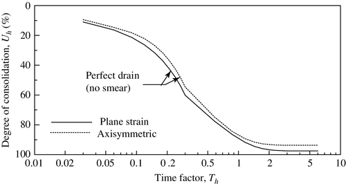
To verify this model, a finite element analysis was undertaken for both axisymmetric and equivalent plane strain models. As an example, a unit drain was analyzed with a drain installed to a depth of 5 m below the ground surface at 1.2 m spacing. The model parameters and soil properties were rw = 0.03 m, rm = 0.05 m, kh = 1 × 10⁻⁸ m/s, and kh′ = 5 × 10⁻⁹ m/s, and the corresponding equivalent coefficients of plane strain permeability were khp′ = 5.02 × 10⁻¹⁰ m/s and khp = 2.97 × 10⁻⁹ m/s based on Eq. (3.30). The water table was assumed to be at the surface and rs = 5rm (based on experimental results). For the elasto-plastic finite element analysis, the MCC model was used as follows: λ = 0.2, κ = 0.04, M = 1.0, ecs = 2, and Poisson’s ratio ν = 0.25, with a saturated unit weight of 18 kN/m3.
The results of both axisymmetric and plane strain analysis are plotted in Fig. 3.14. The average degree of radial consolidation Uh (%) is plotted against the time factor Th for perfect drain conditions. As illustrated, the proposed plane strain analysis agree perfectly with the axisymmetric analysis, with the maximum deviation between the two methods being less than 5%.
Figures 3.15 and 3.16 illustrate the settlements and excess pore pressure variations over time, including smear plus well resistance for a single drain, and again the axisymmetric model and the equivalent plane strain model agreed.
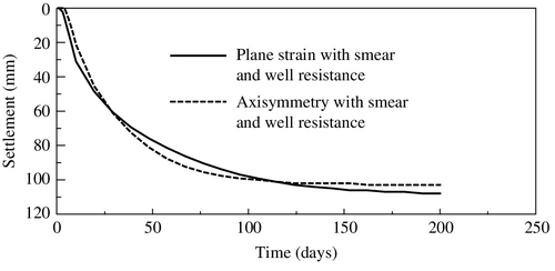
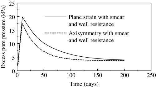
Based on the previous single drain analysis, Figures 3.14 through 3.16 provide concrete evidence that the equivalent (converted) plane strain model is an excellent substitute for the axisymmetric model. In finite element modeling, the 2D plane strain analysis is expected to reduce computational time considerably compared to the time taken by a 3D, axisymmetric model, especially in multidrain analysis.
3.7 Simple 1D modeling of vertical drains
A simple approximate method for modeling the effect of PVD is proposed by Chai et al. (2001). Because PVD increases the mass permeability of subsoil in the vertical direction, it is logical to establish a value for vertical permeability that approximately represents the effect of vertical drainage of natural subsoil and radial permeability toward the PVD. This equivalent vertical permeability (kve) was derived from an equal average degree of consolidation under the 1D condition. To obtain a simple expression for kve, an approximation equation for consolidation in the vertical direction was proposed:
where Tv is the time factor for vertical consolidation, and Cd = constant= 3.54. The equivalent vertical permeability, kve, can be expressed as:
where l is drain length, De the equivalent diameter of unit cell, and
3.8 A finite element model perspective for general design
Finite element analysis is an important tool for current design processes (Potts and Zdravkovíc, 2001). In this section, selected numerical studies have been carried out to study how the embankment slope, construction rate, and drain spacing affect the failure of a soft clay foundation using the finite element code ABAQUS. The subsoil profiles are given in Tables 3.4 and 3.5 and the plane strain permeability coefficients are calculated using Eq. (3.30).
Table 3.4
Soil properties used in finite element analysis
| Depth (m) | Soil type | kh (10–9 m/s) | eo | λ | κ | v | M | γ(kN/m3) |
| 0–2.0 | Weathered clay | 30.1 | 1.8 | 0.3 | 0.03 | 0.3 | 1.2 | 16.0 |
| 2.0–8.5 | Very soft clay | 12.7 | 2.8 | 0.73 | 0.08 | 0.3 | 1.0 | 14.5 |
| 8.5–10.5 | Soft clay | 6.02 | 2.4 | 0.5 | 0.05 | 0.25 | 1.2 | 15.0 |
| 10.5–13.0 | Medium clay | 2.55 | 1.8 | 0.3 | 0.03 | 0.25 | 1.4 | 16.0 |
| 13.0–18.0 | Stiff clay | 0.60 | 1.2 | 0.1 | 0.01 | 0.25 | 1.4 | 18.0 |
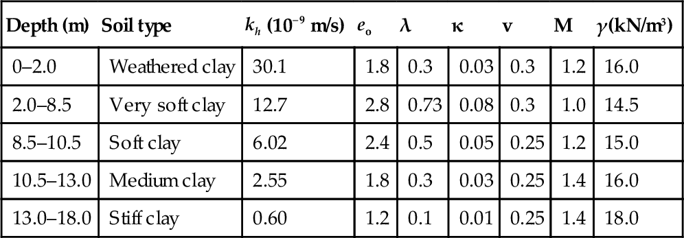
Table 3.5
In situ stress condition used in finite element analysis
| Depth (m) | σho′(kPa) | σvo′(kPa) | u (kPa) |
| 0 | 5 | 5 | − 5 |
| 0.5 | 8 | 8 | 0 |
| 2 | 11 | 11 | 15 |
| 8.5 | 28 | 39.75 | 80 |
| 10.5 | 35 | 49.75 | 100 |
| 13.0 | 49 | 64.75 | 125 |
| 15.0 | 57 | 80.75 | 145 |

3.8.1 Element types for soil and soil–drain interface
The types of elements used in consolidation analysis in the finite element code ABAQUS are shown in Fig. 3.17. The basic element type is a 4-node bilinear displacement and pore pressure element (CPE4P) consisting of 4 displacement and pore pressure nodes at the corners. The higher order of this element is a 20-node triquadratic displacement and trilinear pore pressure nodes with reduced integration (C3D20RP), which contain 20 displacement nodes and 8 pore pressure nodes. As explained by Hibbitt and Sorensen (2004), reduced integration elements use a lower order of integration to form element stiffness. ABAQUS recommends using reduced integration elements because it usually gives more accurate results and is less time consuming than full integration. The common element type used in the analysis presented here is the CPE8RP element, which contains 8 displacement nodes and 4 pore pressure nodes.
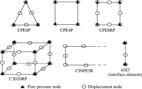
Interface elements are most appropriate to simulate soil–drain interaction. Because the thickness of PVD is relatively small compared to its spacing, the interface element is envisaged as the soil element having properties similar to the adjacent soil except for permeability. A three-node interface element (ASI3) is shown in Fig. 3.17, where there are two pore pressure nodes at the ends.
In finite element analysis, the pore pressure shape function is usually one order less than the displacement shape function. In most of the elements shown in Fig. 3.17, the pore pressure shape function is linear, while the displacement shape functions are either quadratic or cubic.
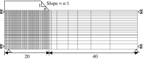
Figure 3.18 presents a typical discretized finite element mesh, which is used for numerical analysis, where only one-half of the embankment is considered by symmetry. A foundation depth of 15 m was considered sufficient for analysis, assuming the existence of a stiff clay layer beneath this depth. The mesh consists of more than 1000 CPE8RP elements and the vertical drains are modeled by an interface element (ASI3). A finer mesh was employed for the zone beneath the embankment, with a half-width of 20 m. The embankment loading is simulated by applying incremental vertical loads.
3.8.2 Embankment constructed on soft clay without any improvement
Effect of the slope of the embankment
To illustrate the effect of embankment slope on foundation failure, two plane strain finite element analyses were conducted using the finite element mesh shown in Fig. 3.18. Two slopes are considered here, 2:1 and 3:1 (horizontal:vertical), and the loading is simulated by a constant rate of 0.1 m/week. Failure is identified when the solution fails to converge and displacement continues to increase without any further load added.
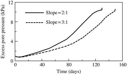
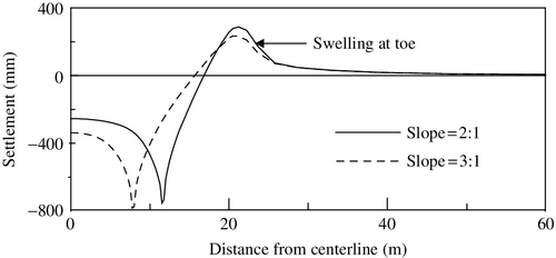
Figure 3.19 shows the predicted heave at the toe of the embankment based on the two models. A measurable change in settlement rate close to failure is observed and, finally, settlement increases without having to increase the embankment height. The decrease in embankment slope has the effect of increasing the embankment height at failure from 1.8 to 2.1 m. Figure 3.20 presents excess pore pressure distribution at 2 m below ground level at the embankment toe. As expected, excess pore pressure increment is not gradual and a sudden increase is observed because the point considered here is located within the expected failure zone. Predicted surface settlement profile at failure based on these two models is presented in Fig. 3.21.

Effect of loading rate of the embankment
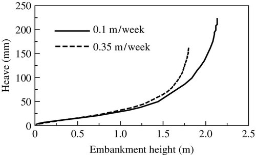
To study the effect of construction rate of the embankment on failure height, plane strain finite element analysis was conducted for the two different construction rates, 0.1 m/week and 0.35 m/week, for an embankment slope of 3:1. The predicted heave at the toe of the embankment is shown in Fig. 3.22. The slow rate of construction permits a greater embankment height at failure, because this gradual rate of construction allows the soft clay to gain shear strength after pore pressure dissipation.
3.8.3 Influence of drain spacing
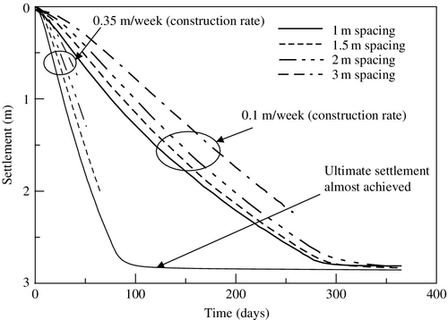
To investigate the effect of vertical drains on embankment stability, four different drain spacings were considered in the analysis: 1, 1.5, 2, and 3 m. The embankment is raised to a maximum height of 4 m, with two different construction rates: 0.1 m/week and 0.35 m/week. The slope of the embankment is assumed to be 2:1.
Figures 3.23 and 3.24 show the predicted surface settlement at the centerline and toe of the embankment, respectively. For a construction rate of 0.1 m/week, impending failure is not noticed for a small drain spacing of up to 2 m, which suggests that the higher dissipation of pore pressure and slower construction rate allow the soft clay foundation to gain sufficient strength to support a 4 m high embankment. If the construction rate is increased to 0.35 m/week, the foundation stabilized with PVD at 1 m spacing reaches its ultimate settlement within a shorter period (100 days) compared to a construction rate of 0.1 m/week (300 days). It is not possible to reach the final embankment height of 4 m if the drain spacing is 1.5, 2, or 3 m (Fig. 3.24b).

3.9 Performance of test embankments constructed on soft marine clay in malaysia
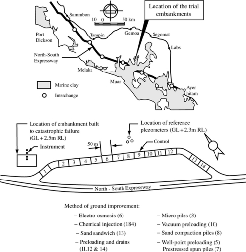
To study the performance and cost effectiveness of various ground improvement methods, in 1986 the Malaysian Highway Authority constructed a series of 15 trial embankments in Muar clay with 9 different ground improvement techniques. The site of the test embankment is about 500 km east of Malacca on the southwest coast of Malaysia (Fig. 3.25). The finite element program ABAQUS is used to predict the behavior of two of these embankments; one without any foundation improvement (i.e., north of embankment #1 in Fig. 3.25), the other with geosynthetic vertical drains (PVD) at 1.3 m spacing installed in a triangular pattern (i.e., #14 in Fig. 3.25).
3.9.1 Embankment constructed to failure
An embankment built for catastrophic failure is shown in Fig. 3.25, located just north of embankment #1. The cross section of the embankment, showing the key instruments with subsoil variation and the discretized finite element mesh, is shown in Figures 3.26 and 3.27, respectively. The piezometers P5 and P6 and the inclinometers I3 and I4 are used to monitor embankment failure. The embankment was raised with a fill material of 20.5 kN/m3 bulk unit weight at a constant rate of 0.4 m/week (Indraratna et al., 1992). The MCC parameters and the in situ stresses are given in Tables 3.6 and 3.7, respectively.
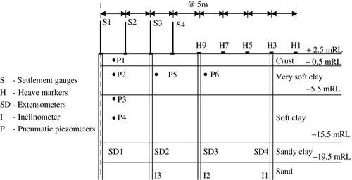

Table 3.6
Soil parameters used in finite element analysis
| Depth | k | λ | ecs | M | v | γs (kN/m3) | kh (m/s) | kv (m/s) |
| 0–2.5 | 0.05 | 0.13 | 3.07 | 1.19 | 0.3 | 16.5 | 1.5 × 10⁻⁹ | 0.8 × 10⁻⁹ |
| 2.5–8.5 | 0.05 | 0.13 | 3.07 | 1.19 | 0.3 | 15.5 | 1.5 × 10⁻⁹ | 0.8 × 10⁻⁹ |
| 8.5–18.5 | 0.08 | 0.11 | 1.61 | 1.07 | 0.3 | 15.5 | 1.1 × 10⁻⁹ | 0.6 × 10⁻⁹ |
| 18.5–22.5 | 0.10 | 0.10 | 1.55 | 1.04 | 0.3 | 16.0 | 1.1 × 10⁻⁹ | 0.6 × 10⁻⁹ |
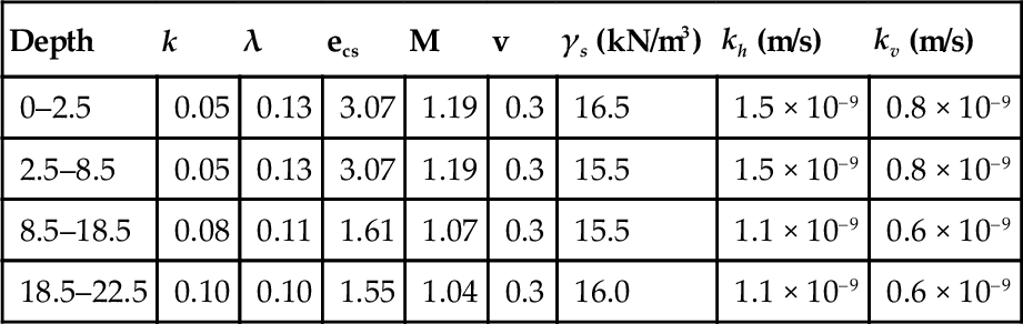
Source: Indraratna and Sathananthan (2003).
Table 3.7
In situ stress condition
| Depth (m) | σh0 (kPa) | σv0 (kPa) | u (kPa) | P′c (kPa) |
| 0 | 0 | 0 | 0 | 110 |
| 2.5 | 13.2 | 22.0 | 16.7 | 110 |
| 8.5 | 33.7 | 56.1 | 75.5 | 40 |
| 18.5 | 67.9 | 113.1 | 173.6 | 60 |
| 22.5 | 81.5 | 135.9 | 212.9 | 60 |
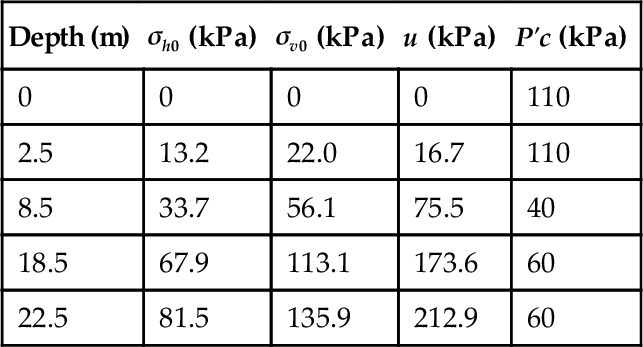
Source: Indraratna and Sathananthan (2003).
The excess pore pressure variation along the embankment centerline, the surface settlement, and the lateral displacement at 10 m from the centerline are plotted in Figures 3.28 through 3.30 for a fill height of 5 m. As expected, the lateral displacement is significantly reduced in the stiffer clay layer. In general, the MCC theory overestimates the lateral displacements. The reason for this discrepancy can be attributed to several factors, including the lateral variability of soil parameters, the use of a simplified associated flow rule, and the effect of the stiff surficial crust (Potts and Zdravkovic, 2001). It was found that lateral displacements are also sensitive to nominal changes of compression parameter λ (Indraratna et al., 1992).

3.9.2 Embankment stabilized with geosynthetic vertical drain
An embankment stabilized with a geosynthetic vertical drain is shown in Fig. 3.25 as embankment #14. The embankment cross section with key instrumentation and the associated subsoil profile is shown in Fig. 3.31. The equivalent drain radius based on Eq. (3.4) is estimated to be rw = 0.03 m and the smear zone radius is taken as rs = 0.15 m. The Cam-clay parameters and equivalent plane strain permeabilities based on Eq. (3.30) are given in Table 3.8. Table 3.9 tabulates the in situ stress distribution. Embankment construction was carried out in two loading stages; during the first 14 days the height was raised to 2.57 m (stage 1) and after a 90-day rest period the height was raised to 4.74 m in 24 days (stage 2).
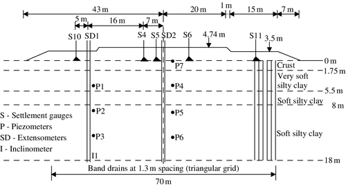
Table 3.8
Soil parameters used in finite element analysis
| Depth (m) | κ | λ | ecs | M | v | γs | Permeability (10–9 m/s) | |||
| kh | k′h | khp | k′hp | |||||||
| 0–1.75 | 0.06 | 0.30 | 3.10 | 1.19 | 0.29 | 15.0 | 6.4 | 3.0 | 2.45 | 0.60 |
| 1.75–5.50 | 0.06 | 0.60 | 3.10 | 1.19 | 0.31 | 15.0 | 5.2 | 2.7 | 1.36 | 0.58 |
| 5.50–8.0 | 0.05 | 0.30 | 3.06 | 1.12 | 0.29 | 15.5 | 3.1 | 1.4 | 0.81 | 0.29 |
| 8.0–18.0 | 0.04 | 0.35 | 1.61 | 1.07 | 0.26 | 16.0 | 1.3 | 0.6 | 0.34 | 0.13 |
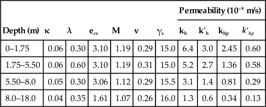
Source: Indraratna and Sathananthan (2003).
Table 3.9
In situ stress condition
| Depth (m) | σv0′ (kPa) | σh0′ (kPa) | u (kPa) | Pc′ (kPa) |
| 0 | 0 | 0 | 0 | 110 |
| 1.75 | 28.6 | 17.3 | 0 | 95 |
| 5.50 | 48.4 | 29.1 | 36.7 | 44 |
| 8.0 | 62.6 | 37.6 | 61.3 | 60 |
| 18.0 | 124.6 | 74.8 | 159.3 | 135 |
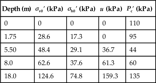
Source: Indraratna et al. (1994).
The finite element mesh of the embankment is shown in Fig. 3.32 and the location of inclinometer (ID1, 23 m away from the centerline) and piezometers are conveniently defined at mesh nodes. The well resistance of the drain was included because it was 18 m long. The well resistance was simulated by considering the vertical permeability of the transformed drain wall, as previously shown in Eq. (3.31c). The equivalent coefficient of permeability of the drain was estimated as 0.0005 m/s by a single drain analysis.

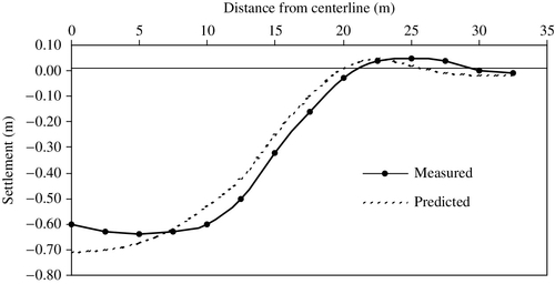
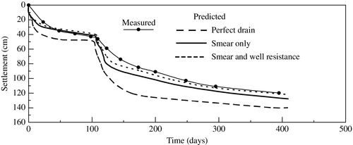
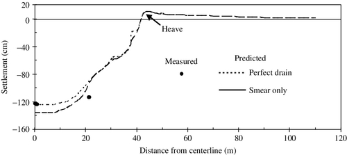
The predicted and measured settlements at the centerline and along the surface are shown in Figures 3.33 and 3.34, respectively. Heave is also predicted beyond the toe of the embankment, that is, at about 45 m away from the centerline, but, regrettably, no field data were available for comparison. The predictions acceptably agree with the limited field measurements obtained near the centerline.
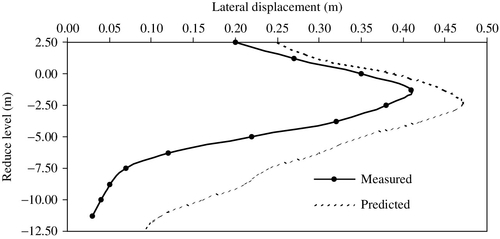
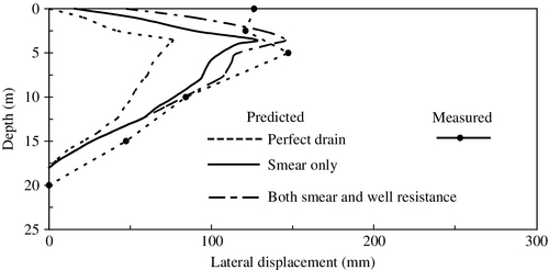
The evaluated and measured excess pore water pressure variations are shown in Fig. 3.35. The measured excess pore pressure does not indicate much dissipation during stage 2 due to the piezometer malfunctioning. Even though the prediction of excess pore pressure is made accurately in stage 1 by including the smear effect, the predicted postconstruction pore pressure only improved slightly by including both smear and well resistance. As expected, the “perfect drain” underestimates the measurements. Observed and predicted lateral deformations are plotted in Fig. 3.36. Acceptable agreement between the field data and predictions is obtained when both the smear and well resistance are considered. The perfect drain condition gives the smallest lateral deformation while maximizing vertical deformation.

3.9.3 Normalized deformation factors
The lateral displacement and settlement can be normalized with respect to the corresponding fill height to examine the effectiveness of the ground improvement techniques. Thus, the following “stability” indicators are defined (Indraratna et al., 1997): β1, the ratio between lateral displacement and the corresponding fill height, β2 the ratio between settlement and the corresponding fill height, and α = β1/β2.
Figure 3.37 shows variation of β1 with depth and Fig. 3.38 shows the variation of α with depth. The normalized displacement of a PVD-stabilized embankment is considerably less than an embankment constructed to failure. These results clearly show that vertical drains effectively decrease lateral deformations and enable the critical height of an embankment to be increased. After 13 days, the untreated embankment fails with unacceptably large lateral displacement (Fig. 3.37). The PVD-stabilized foundation takes more than 7 years before lateral displacement becomes similar to the failed embankment.


The normalized deformation factors for a few trial embankments are also compared in Table 3.10. In comparison with the unstabilized embankment constructed to failure, the stabilized foundations are characterized by considerably smaller values for α and β1, which elucidates their obvious implications on stability. The normalized settlement (β2) on its own is not a proper indicator of instability, but is still a useful stability indicator when taken in conjunction with α and β1. For example, the foundation having SCP gives the lowest values of β1 and β2, clearly suggesting the benefits of sand compaction piles over band drains.
Table 3.10
Normalized deformation factors (modified after Indraratna et al., 1997)
| Ground improvement scheme | a | ß1 | ß2 |
| Sand compaction piles for pile/soil stiffness ratio of 5 (h = 9.8 m, including 1 m sand layer) | 0.185 | 0.018 | 0.097 |
| Geogrids + vertical band drains in square pattern at 2.0 m spacing (h = 8.7 m) | 0.141 | 0.021 | 0.149 |
| Vertical band drains in triangular pattern at 1.3 m spacing (h = 4.75 m) | 0.127 | 0.035 | 0.275 |
| Embankment rapidly constructed to failure on untreated foundation (h = 5.5 m) | 0.695 | 0.089 | 0.128 |

3.10 Conclusion
In this chapter, the use of prefabricated vertical drains, their properties, and associated merits and demerits have been discussed. The behavior of soft clay under the influence of PVD was described on the basis of numerous case histories where both field measurements and numerical predictions were available. A sophisticated 3D multidrain analysis with an individual axisymmetric zone of influence, with smear for each and every drain, will easily exceed computational capacity when applied to a real embankment project with a large number of PVDs. In this context, the equivalent plane strain models will continue to offer a sufficiently accurate predictive tool for design, performance verification, and back-analysis.
Selected numerical studies have been carried out to study the effect of embankment slope, construction rate, and drain spacing on the failure of soft clay foundations. Finally, the observed and the predicted performances of well-instrumented full-scale trial embankments built on soft Malaysian marine clay have been discussed using the plane strain theory. The numerical results based on ABAQUS conclude that the inclusion of both smear and well resistance improves the accuracy of the predicted settlement, excess pore pressures, and lateral deformation. As expected, the perfect drain analysis always overpredicts settlement and underpredicts excess pore pressures. The results presented here reaffirm that the effects of soil disturbance (smear) and well resistance are important for estimating deformation. While an accurate prediction of surface settlement is generally feasible, the acceptable prediction of lateral displacement is often difficult due to inherent assumptions made in the plane strain models. An accurate prediction of lateral displacement undoubtedly depends on the correct assessment of the value of λ of the MCC model, and the discharge capacity of PVD, among other parameters.