
New Analytical Approach for Predicting Horizontal Displacement of Stone Columns
Kim Chan; Bosco Poon GHD, Sydney, Australia
Abstract
This chapter presents an analytical approach for the prediction of both vertical and horizontal displacements of soft ground improved using stone columns in a two-dimensional (2D) finite element analysis (FEA). This involved simulating the stone columns as continuous strips in the FE model with appropriate strip width, spacing, and smeared properties. This approach relies on the selection of appropriate stress concentration ratios between the vertical stress supported by the stone columns and the stress within the surrounding soil.
A parametric study of the various key influencing factors on the stress concentration ratio is presented. Design charts to assess the equivalent 2D column stress concentration ratios are provided for the design of both fully penetrating columns and floating columns.
The accuracy of the proposed 2D strip model was investigated by comparing the results with the baseline 3D analysis, axisymmetric FEA, and conventional 2D FEA approach using equivalent blocks. It was found that all approaches estimated reasonably similar settlement. However, the conventional 2D equivalent block method tended to underestimate horizontal displacement. The proposed 2D strip model is therefore preferable over the conventional 2D approach using composite block material to represent the entire improved soil, particularly when horizontal displacement or edge deformation is important in the design.
To validate the new analytical approach, this method of analysis was used to compare with the results of a full-scale trial pad loading test on an area installed with working stone columns. Both settlement and horizontal displacement were predicted and compared with monitoring results. In addition, vertical stresses at different locations at the original ground surface level were assessed using load cell monitoring results. The comparison showed that the new analytical approach agrees well with the monitoring results and thus seems to confirm the appropriateness of the new analytical method for practical design applications.
18.1 Introduction
Stone column installation is considered an effective and low-cost ground improvement technique for the support of structures and embankments founded on soft soils. It is believed that one of the earliest known stone column applications was the construction of the Taj Mahal in India in the 1650s. In more recent times, the stone column technique was used as a ground-strengthening system in 1830 in France for military purposes (Hughes et al., 1975). The modern-day stone column system installed using a vibratory technique was introduced in 1939 by Steuermann. Since then, the installation method has been refined with the procedure controlled and monitored using computers.
The basic concept of stone column installation involves creating vertical holes in the ground and filling them with compacted granular materials such that the surrounding soft ground is strengthened. Nowadays, the construction of stone columns typically uses two main installation techniques, namely the vibro-replacement method using the wet, top-feed approach and the vibro-displacement method using the dry, bottom-feed approach. It is important to note that the stone columns thus created do not behave as structural elements like some other columnar systems formed using concrete or cement grout.
While the compacted granular materials usually have significantly higher shear strength than the surrounding soils, the columns do not exhibit any discernible structural capacity such as bending and tension. As a result, stone columns should not be designed as structural members, but should be treated as soil elements. The design approaches for stone columns are therefore somewhat different to other columnar ground improvement systems and require special consideration when designing them to improve soft ground.
18.2 Conventional design approaches
The stone column technique is conventionally used to improve the bearing capacity of the ground and to reduce both total and differential settlements when the ground is loaded. Because the columns are created using compacted granular materials, they are also effective in reducing the liquefaction potential of the treated ground and in accelerating the rate of consolidation of the surrounding soft soils by acting as vertical drains.
As the stone columns are usually significantly stiffer than the surrounding soils, most of the applied load to the ground will be taken by the stone columns instead of the surrounding soft soils because of strain compatibility. If the superimposed load is applied via a relatively rigid slab, the settlement and vertical strain between the rigid slab and the soft soils should be similar. In this instance, the ratio of the load carried by the columns to the load carried by the soft soils should be roughly proportional to the stiffness ratio between the stone columns and the soft soils.
Conversely, if the stone columns are used to support a relatively flexible embankment, the load distribution will be dependent on the amount of soil arching between columns, which is a function of the spacing of the stone columns. Furthermore, the soft soils surrounding the stone columns will settle slightly more than the stone columns. The additional load applied to soft soils will cause some consolidation of the soft soils. As the soft soils consolidate, some of the load will be transferred to the adjacent stone columns which in turn will cause settlement of the stone columns, leading to some load transfers back to the soft soils. This process will continue until some equilibrium is reached.
When the stone columns are loaded and settle, they deform in shape, which could cause bulging of the stone columns, particularly at the top sections of the columns where the stresses within the columns are higher. With no or limited lateral support, the stone columns will fail in bulging and shearing. As a result, stone columns are more effective when they are installed in soils with some reasonable shear strength, typically with undrained shear strength, su of at least about 20 kPa. The methods generally used to design and analyze stone columns range from semiempirical methods to simple theoretical approaches (e.g., Balaam and Booker, 1983) to 2D and 3D finite element analysis (FEA).
Because many applications using stone columns are intended to reduce settlement and to improve bearing capacity, most of the design methods have been developed and calibrated with vertical loading. This includes the so-called “unit cell” concept where one column and its tributary area of surrounding soil is treated as a unit cell. The behavior of the stone column and the unit cell can then be analyzed as either elastic materials or as elastoplastic materials (e.g., Balaam and Booker, 1981; Balaam and Booker, 1983).
Using the unit cell concept, a number of design approaches have been proposed by various researchers (e.g., Priebe, 1995, Balaam and Booker, 1983). Generally, these approaches have been calibrated using full-scale field tests and/or laboratory tests. They have been proven to give reasonable predicted settlement of soft ground treated with stone columns.
Alternatively, some designers have adopted finite element analytical (FEA) methods to analyze and design stone columns (e.g., Kundu et al., 1994). Typically, the stone-column-treated soft ground is modeled as a homogenous material with equivalent composite properties adopted based on the soft soil properties and the stone column design (e.g., diameter, spacing, properties of stone). When appropriate equivalent composite properties are used, the settlement prediction seems to be reasonably accurate.
Recently, some researchers (e.g., Tan et al., 2008) have started to simulate rows of stone columns using equivalent plane-strain strips in FEA modeling. This approach is considered more appropriate when variable column spacing is adopted or when differential settlement is critical.
It is reiterated that the previously discussed design methods mainly deal with vertical loading. However, when stone columns are used for slope stabilization (e.g., Vekli et al., 2012) or when lateral displacement is critical in the satisfactory performance of the development, the previously mentioned approaches and simplifications may no longer be applicable.
In recent years, the authors of this chapter have carried out research to develop an appropriate FEA method to analyze stone columns subjected to lateral loading (e.g., Chan et al., 2007; Chan and Poon, 2012; Poon and Chan, 2013). This FEA approach using equivalent 2D strips is described in detail in the following.
18.3 Idealized 2D modeling approach
For the modeling of stone columns in 2D FEA, the width of the equivalent strips can be made to be equal to the width of an equivalent square of the cross-sectional area as shown in Fig. 18.1. The spacing of the strips is equal to the actual spacing of the stone columns, s, for square arrangement and ![]() for equilateral triangular arrangement. A Mohr–Coulomb model is used for the assessment of strength capacity of stone columns with Poisson’s ratio of 0.3. The equivalent Young’s modulus Eeq and cohesion ceq of the strips can be calculated based on weighted average approach as given by Eq. (18.1).
for equilateral triangular arrangement. A Mohr–Coulomb model is used for the assessment of strength capacity of stone columns with Poisson’s ratio of 0.3. The equivalent Young’s modulus Eeq and cohesion ceq of the strips can be calculated based on weighted average approach as given by Eq. (18.1).

where Asoil and Acolumn are the areas of the soil and column inside a unit cell within the 2D strip, as shown in Fig. 18.1.
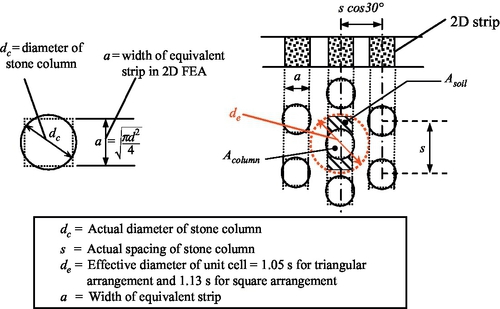
The equivalent friction angle, ϕeq, of the strips can be derived based on a force equilibrium approach as given by:

where ϕsoil is the friction angle of the soil and ϕcolumn is the friction angle of the stone column. The determination of ϕeq requires a presumption of stress concentration ratio, n, which is defined as the ratio of the average applied vertical stress within stone column to the average applied vertical stress of the surrounding soil at the same level. Section 18.4 presents an appraisal for this parameter. Note that the present 2D FEA is an elasto-plastic analysis in which the decay of excess pore pressure with time was not taken into account.
18.4 Stress concentration of stone columns under flexible embankment loading
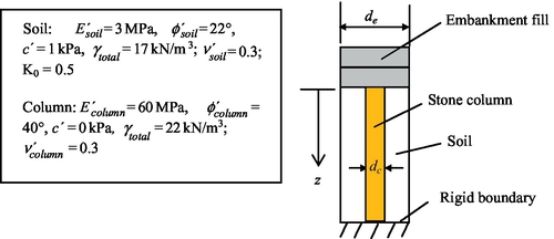
This section presents a series of elasto-plastic solutions in charts for the stress concentration ratio, n, of stone columns founded on (1) rigid boundary and (2) infinite compressible soil materials. The solutions were obtained based on axisymmetric FEA using PLAXIS software for a “unit cell” consisting of a stone column and the surrounding soil within a column’s zone of influence. Interface elements were introduced at the soil–column contact to allow for potential slippage. The interface strength was assumed to be 70% of the original soil strength (Rint = 0.7 in PLAXIS). Note that the interface properties have minimal effect on the results as the stone column is in triaxial state.
18.4.1 Stone columns on rigid base
Figure 18.3(b) presents the calculated n with depth for a particular case where embankment load is applied on stone columns that are founded on a rigid base. The selected column configuration and parameters for the axisymmetric “unit cell” analysis are shown in Fig. 18.2. In particular, the ratio of the effective diameter of the unit cell to the column diameter, de/dc, is 2. Additionally, the embankment fill was modeled as soil elements, and the arching stresses developed above the column have been accounted for in the FEA model.
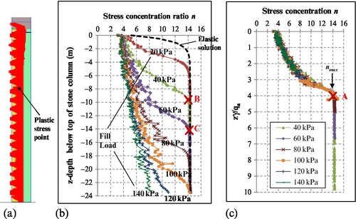
If the column and soil were appraised as elastic materials, the calculated n (dashed line in Fig. 18.3(b)) increases from 5 at the top of column, which is consistent with the value obtained from design chart given in FHWA (1983) for embankment supporting columns, to about 14 at depth, which is commensurate with the equal strain solution (soil and column settle at the same rate at depth) given by Balaam and Poulos (1982).
When the column and soil are modeled as Mohr–Coulomb materials, yielding elements begin to form at the column top after a small load (~ 20 kPa) is applied, leading to a reduction in stress concentration. The yielding of the column (thus the reduction of n) progresses downward through the column as the applied load level increases, as shown by the solid curves in Fig. 18.3(b). Note that the oscillatory trend of the curves is due to some instability of the numerical solution, which is common for the current adoption of highly non-associated flow rule (dilation angle ψ = 0°) in the Mohr–Coulomb model (Carter et al., 2005). Figure 18.3(a) shows the stress state of the unit-cell model after the application of maximum embankment load. This figure indicates that most yielding elements are confined within the column periphery. The soil is generally elastic and therefore the soil friction angle has little influence on the solution.
Figure 18.3(c) shows a normalized plot in which the depth of the column, z, was normalized by qa/γ, where qa is the applied fill stress and γ is the total unit weight of the soil. It is found that the normalized stress concentration curves for the different load levels (≥ 40 kPa) lie on a single curve. The turning point of the normalized curve corresponds to the transition from the upper yielded zone to the lower nonyielding zone, which occurs at different z for the different qa. For example, point A in Fig. 18.3(c) occurs at z · γ/qa = 4. When qa = 40 kPa and γ = 17 kN/m3, z = 9.5 m (i.e., point B in Fig. 18.3(b)). When qa = 60 kPa, z ≈ 14 m (i.e., point C in Fig. 18.3(b)).
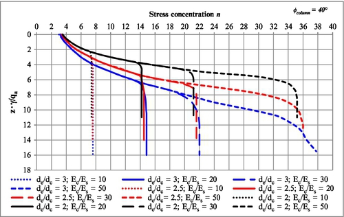
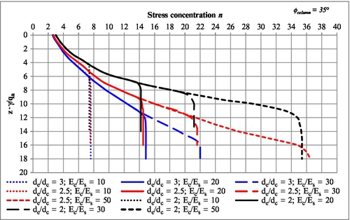
Figures 18.4 through 18.6 presents a series of normalized curves for the n value under different modulus ratios, de/dc ratio, and friction angles of the stone column, ϕcolumn. For a given de/dc ratio and ϕcolumn, the stress concentration is higher for higher modulus ratio Ecolumn/Esoil (denoted as Ec/Es in the figures). Conversely, for the columns with a given modulus ratio, the extent of the yielding zone, and thus the reduction of stress concentration, is greater as de/dc ratio increases even though the maximum stress ratio in the columns (elastic condition) is ultimately similar. This occurs because there is less lateral confinement for the spaced columns, leading to greater yielded zone and stress reduction within columns. A comparison of the corresponding curves in figures shows that the loss of stress concentration due to yielding is more severe for column material having a lower ϕcolumn.

18.4.2 Stone columns on compressible soils: elastic appraisal
For stone columns founded on rigid base, it can be expected that the surrounding soil generally settles more than the stiffer stone columns. Conversely, for stone columns founded on compressible soil, the FE solution based on elastic model has indicated that there exists a lower equal settlement plane below which the columns move more than the soil to mobilize positive skin resistance of the soil. This has resulted in a greater load transfer from the column to the surrounding soil and therefore the stress concentration ratio, n, reduces (see Fig. 18.7(a)).
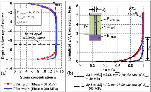
Figure 18.7(b) shows a plot of normalized distance from the column base y/dc versus stress concentration reduction ratio r (= n/nmax) for the corresponding elastic FE solutions given in Fig. 18.7(a), where y and dc are defined in the inset in Fig. 18.7(b); and nmax is the maximum computed n value based on elasticity, as shown in Fig. 18.7(a). The FEA results for r near the column base can be approximated by the following logarithmic relationship.
where ξ is the influenced zone (also normalized by the column diameter dc) that is measured from the base of the column to the equal settlement plane. The magnitude of m controls the rate of reduction of r with y/dc. The higher the m, the more rapid reduction of r would be toward the column tip.
Figure 18.7(b) indicates that as the Young’s modulus Ebase of the soil beneath the columns increases, the extent of ξ reduces. Also, the ratio r reduces more rapidly toward the tip of the column (i.e., m increases) as Ebase increases. Figure 18.8 presents the computed ξ and m for the different Ebase/Ecolumn and Ebase/Esoil ratios based on linear elasticity finite element analyses. The following points can be drawn:

• The influenced zone ξ at the column base reduces as Ebase/Ecolumn increases. The reduction may be approximated by linear ξ – log(Ebase/Ecolumn) relationships as delineated by curves 1 and 4 in Fig. 18.8(a) for de/dc ratio of 3 and 2, respectively. A curve in-between representing de/dc ratio of 2.5 has not been shown for clarity of the figure. Note that these curves can apply to cases where Ebase/Esoil ≥ 10 as Esoil has negligible effect on the shape of r under this condition. For a particular de/dc ratio, ξ shows a lower value as Ebase/Esoil reduces to less than 10, although the trend of reduction with log(Ebase/Ecolumn) remains linear and parallel with that for Ebase/Esoil ≥ 10 (curves 2 and 3, 5, and 6 in Fig. 18.8(a)).
• The rate of reduction of r toward the column tip, represented by the parameter m, has been found to increase linearly with Ebase/Ecolumn. Curve 7 in Fig. 18.8(b) shows such relationship and is applicable for cases with different de/dc ratio up to 3 (limit of parametric range) and with Ebase/Esoil ≥ 10. Curves 8 and 9 delineate the corresponding curves for cases with Ebase/Esoil = 2 and 1, respectively.
18.4.3 Stone columns on compressible soils: elastoplasticity
The effect of compressible base on stress concentration ratio, n, is now discussed based on a linearly elastic–perfectly plastic Mohr–Coulomb model. In particular, the soils surrounding and below the stone columns have been appraised separately using (1) effective shear strength (c′, ϕ′) and (2) undrained shear strength su.
Figure 18.9(a) shows the computed n under different fill loads for the same case as in Fig. 18.2, except that the column is founded on compressible soil that is represented by c − ϕ materials. The stress concentration curves initially follow identical paths as those shown in Fig. 18.3(b) until they intercept the lower equal settlement plane and thereafter trace along the curve of the elastic solution at the column base. To explain the stress transfer mechanism, the material stress state of the model at the end of simulation (under 140 kPa fill stress) is presented (inset in Fig. 18.9(a)). As before, yielding of the column follows a top-down process. While there is significant yielding of the column due to high stress ratio, there is little yielding in the surrounding soil, especially toward the column base because of sufficient confinement even with an adopted soil friction angle as low as 22°. Because the soil is elastic, the reduction of n due to the compressible elastic base soil can be superimposed directly onto the aforementioned reduction due to yielding of column.
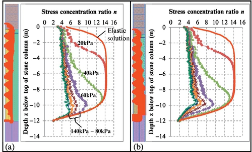
Figure 18.9(b) presents the results for the case where su = 30 kPa has been adopted for the soils surrounding and below the column. Significant yielding occurs in the soils, which has altered the shape of the stress concentration curves toward the column base as compared to that of the c − ϕ soils. However the differences are not great and for the purpose of assessing n, the problem can be idealized by assuming that there is no failure in the surrounding soil so that its behavior is essentially elastic.
18.4.4 Procedure for assessing stress concentration
The following procedure for assessing the stress concentration of the stone columns under fill embankment may be proposed:
Step 1 – Assess the stress concentration ratio, n, along column depth by using charts given by Figs. 18.4 through 18.6, which have accounted for, in a 3D sense, the load transfer mechanism between stone columns and the surrounding soil with depth. The charts developed herein provide solutions of n under different column spacing (i.e., de/dc ratio), ratios of column to soil moduli (Ecolumn/Esoil), and friction angles of the stone column.
Step 2 – Assess the influence of the compressible base soil on n, based on elasticity by the following equation:
where r is the stress concentration reduction ratio given in Eq. (18.4), which is a function of ξ and m given in Fig. 18.8; and nmax is the maximum elastic n value below the turning point of each normalized z · γ/qa–n curve in Figures 18.4 through 18.6.
Step 3 – Superimpose the solution for below the equal settlement plane from Step 2 onto that of Step 1. Thereby, the final n along the depth of the column is the lower of the two solutions at the same depth.
18.5 Modeling of fill embankment over soft clay treated with stone columns
The accuracy of plane-strain idealization of stone columns using equivalent strips in 2D FEA was investigated under self-weight load imparted by a 6-m-high embankment with 2H:1V batter. The analyses undertaken for the investigation include:
• Analysis 1: Full 3D FEA of embankment over stone columns modeled by solid elements
• Analysis 2: Axisymmetric FEA of a unit cell consisting of one stone column
• Analysis 3: 2D plane-strain FEA with the stone columns modeled as strips
• Analysis 4: 2D FEA with the entire soil and columns modeled as equivalent block
Table 18.1 summarizes the adopted parameters for all analyses. The full 3D FEA (Analysis 1) is considered a baseline model that comprises a 13-m-long segment of embankment over soft clay foundation treated with stone columns in a triangular grid formation. The analysis was repeated with the 0.9-m-diameter stone columns spaced at 1.7 m, 2 m, and 2.5 m. The 3D FE mesh is shown in Fig. 18.10. Only half of the embankment segment was modeled because of symmetry. The 3D FEA utilizes solid elements (15 nodes wedge element) for stone columns and interface elements at the column–soil contact. Two cases of interface strength of 100% and 67% of the surrounding soil strengths have been considered.
Table 18.1
FEA model parameters for stone column
| Analysis (1) (2) | Column spacing s (3) (m) | Ratio of unit cell diameter to column diameter de/dc | Area replacement ratio ar | Stone Column Parameters | Comment |
| 1,2 - baseline FEA | 1.7, 2, 2.5 | 2.0, 2.3,2.9 | 0.26, 0.19, 0.12 | E′col = 50 MPa, c′col = 0kPa, ϕ′col = 40º | − |
| 3 - 2D FEA with strips | 1.7 | 2.0 | 0.26 | E′strip = 26 MPa, c′strip ~ 1kPa, ϕ′strip = 37º | Stress concentration ratio n ≈ 4 − 5 |
| 2 | 2.3 | 0.19 | E′strip = 22 MPa, c′strip ~ 1kPa, ϕ′strip = 35º | Stress concentration ratio n ≈ 4 | |
| 2.5 | 2.9 | 0.12 | E′strip = 18 MPa, c′strip ~ 1kPa, ϕ′strip = 33º | Stress concentration ratio n ≈ 3.5 − 4 | |
| 4 - 2D FEA with equiv. block | 1.7 | 2.0 | 0.26 | E′block = 6 MPa, c′block ~ 1kPa,ϕ′block = 30º | − |
| 2 | 2.3 | 0.19 | E′block = 6 MPa, c′block ~ 1kPa, ϕ′block = 30º | − | |
| 2.5 | 2.9 | 0.12 | E′block = 6 MPa, c′block ~ 1kPa, ϕ′block = 30º | − |

Notes to Table 18.1:
(1) Properties of soil surrounding the columns are E′soil = 3 MPa, c′soil = 2kPa, ϕ′soil = 26º.
(2) Properties of soil beneath the columns are E′base = 30 MPa, c′soil = 5kPa, ϕ′soil = 28º.
(3) Stone columns in triangular arrangement.

The axisymmetric 3D FEA (Analysis 2) is also considered as a baseline model for embankment settlement under axially axisymmetric loading condition that occurs in the zone away from the embankment batter. The influence radius of the axisymmetric unit cell was varied, so as to be equivalent to the actual spacing as adopted in the full 3D Analysis 1.
In Analysis 3, a 2D plane-strain idealization of the stone columns using equivalent strips was investigated. The strips are divided into several segments, each of which has different strength properties that correspond to the varying stress concentration along the column depth. The dimension and spacing of the 2D strips and their equivalent properties were derived as per the procedure outlined in Section 18.4 and stress concentration ratio from Figs. 18.4 through 18.6.
Analysis 4 presents the conventional 2D approach in which the entire treated soil is represented by a single block with the equivalent strengths, ϕ block, c block, and Young’s modulus E block derived based on a semiempirical relationship given by Madhav and Nagpure (1996):

In the preceding equations, ar is the area replacement ratio and is defined as the ratio of the cross-sectional area of one column to the total area of the unit cell.
Before considering the numerical results in detail, it is illuminating to discuss the deformation mechanism of the stone columns under the loading of a flexible fill embankment. Figure 18.11(a,b) indicate that the deformation of the stone columns as given by the 2D strip model (Analysis 3) is similar to that of the baseline 3D (Analysis 1) result, in which the stone columns can be broadly divided into three zones: Zone 1 away from the fill batter where columns underwent vertical deformation by “bulging”; Zone 2 just behind the crest of the fill batter where columns underwent both vertical and horizontal deformation by “bulging” and “leaning”; and Zone 3 beneath the fill batter where columns underwent mainly leaning. This numerical prediction for the deformation appears to be consistent with the results of the centrifuge model test carried out by Stewart and Fahey (1994) for a stone column foundation system supporting a stockpile and railway embankment.
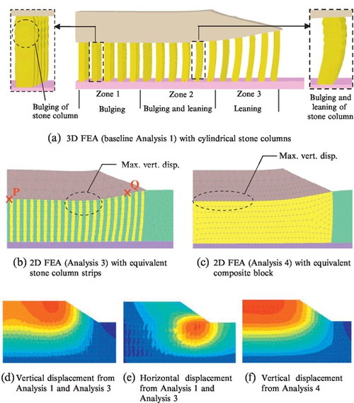
In Zone 1 away from the fill batter, the stone columns are subject to axially symmetric loading conditions and thus the axisymmetric FEA (Analysis 2) is also considered applicable as the baseline solution for this zone. In Zone 2 just before the crest of the fill batter, it can be observed from the FEA results (see Fig. 18.11(b,d)) that stone columns exhibit the greatest vertical displacement (more than those at Zone 1). This is presumably due to the concurrence of the bulging and leaning deformation mechanisms of the stone columns. Conversely, the columns in Zone 3 exhibit a maximum horizontal displacement mechanism (Fig. 18.11(e)) and this is likely due to the prevailing leaning deformation of the stone columns.
Figure 18.11(c) presents the deformation mechanism given by the 2D FEA using the conventional composite block material (Analysis 4). This method is unable to capture the bulging and leaning deformation of the stone columns. The maximum vertical displacement is predicted to occur at the center of the embankment (i.e., at Zone 1; refer to Fig. 18.11(f)), as opposed to occurring in Zone 2 as predicted by the baseline 3D FEA (Analysis 1) and the proposed 2D FEA approach using equivalent strips (Analysis 3).
Figure 18.12(a) shows a plot of predicted settlements at point P versus area replacement ratio ar. All analyses give comparable results, indicating that all the different FE methods are commensurable in terms of settlement prediction under axially symmetric load condition. Figure 18.12(b) presents the predicted horizontal displacement at point Q. The following points are drawn from the results:

• When original soil strengths are used for the interface properties, the result of the 2D strip model (curve 2) compares well with that of the 3D baseline model (curve 1). Both results show a trend of reducing horizontal displacement with ar.
• When the interface strength of the columns in the 3D model are reduced to 67% of the soil strengths, the result (curve 3) indicates an initial drop-off in horizontal displacement with ar, but increases again once ar > 20%. This is due to increasing proportion of yielding elements in the remolded soil as the columns draw closer to each other.
• The application of the same interface strength reduction (67% of surrounding soil strength) in the 2D equivalent strip model has caused excessive yield in the remolded soil and led to increased horizontal displacement with ar (curve 4). A better fit to the 3D solution is by changing the interface strength to 80% of the surrounding soil strength (curve 5). Evidently, there needs a regime to determine an equivalent interface strength for the strip model. This merits further research.
• The 2D block model result (curve 6) underpredicts the horizontal displacement when compared with the 3D baseline model predictions. This indicates that the use of isotropic soil properties in the 2D block model, which were derived based on semiempirical relationships originally for settlement prediction under axially loading condition, have overestimated the reduction in lateral spreading underneath the embankment batter. The use of equivalent strips in the 2D strip model is able to capture the interaction between the soil and the stone column, leading to a better agreement with the lateral deformation prediction from the 3D baseline solution.
18.6 Instrumented trial embankment on stone-column-treated soft ground at kooragang island
18.6.1 Background
Kooragang Island is located on the lower reaches of the Hunter River in Australia and comprises an island about 10 km × 3 km that has been formed by reclamation of a number of former smaller islands, channels, and shallows. The Hunter River splits into the north and south arms on either side of the island.
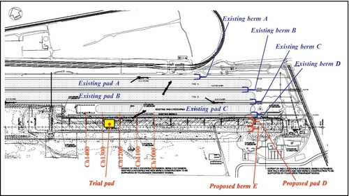
The Kooragang Coal Terminal is located on the southeastern portion of the island, a reclaimed swamp land underlain by soft soil sediments. The facilities allow unloading of coal brought in by rail and storage of the coal until transfer to ship-loading facilities on the south arm of the Hunter River. All of the coal delivered to Kooragang is stored in the stockpiling areas located on the northern edge of the terminal. To increase coal export capacity from 90 to 102 MPa, the coal terminal has undergone expansion including the construction of an additional stockyard and a new machinery berm. The new expansion was sited to the south of and parallel to the existing stockpile area—that is, stockpile pads A to C and berms A to D for machinery as shown in Fig. 18.13. The new area is designated as pad D and berm E.
In general, the proposed site was preloaded to reduce postconstruction settlement. However, it was known that the depth of soft clay increased on the eastern and western ends of the new areas. Given the planned commencement dates for coal export, there was insufficient time to consolidate these areas under preload and, thus, a ground improvement solution using vibro-replacement stone columns was adopted to treat the eastern and western sections of the new stockyard. Refer to Chan et al. (2007) for the details of stone column design at Kooragang site.
One key aspect of the design was to satisfy the extremely stringent postconstruction displacement criteria for machinery operation considerations. To verify the design, a trial embankment load test was conducted on working columns in the region of the deepest soft clay zone. The trial embankment was instrumented and was monitored for a period of about two months to assess the performance of the stone columns under the trial embankment loading.
This section presents the measured stress distribution, settlements, and horizontal displacements at the trial embankment, and compares with those predicted by 2D FEA using the equivalent strip method.
18.6.2 Subsoil conditions
The basic site stratigraphy comprises a layer of about 3-m-thick very dense sand fill, underlain by a 2 to 4.5-m-thick layer of very soft to soft alluvial clay, over a lower dense alluvial sand horizon. A deep clay unit underlying the lower sand was also encountered in certain sections of the stockyard site. However, for the stone column design purposes, the presence of the deep clay is considered to be of secondary importance only. The upper sand fill and soft clay units are of particular interest for assessing the performance of the stone columns.
The Atterberg limits shown in Fig. 18.14 indicate that the very soft to soft alluvial clay is highly plastic with average LL and PI values of 80 and 54, respectively. The average moisture content and the bulk unit weight are 69% and 15.5 kN/m3, respectively.
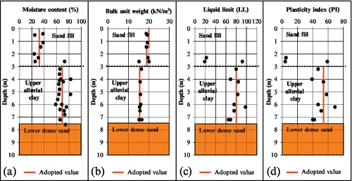
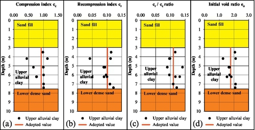
Figure 18.15 presents the compression index (cc), recompression index (cr), cr/cc ratio, and the initial void ratio (eo) versus depth for the available alluvial clay data. Most of the cc data points lie within 0.8–1.1 and the cr values within 0.012–0.026. The cr/cc ratios lie within a range of 0.09–0.14, which is consistent with published typical values. The eo range of the clay is 1.5 to 2.1. For the current assessment, the adopted mean values of cc and cr values are 0.92 and 0.10, respectively. Using a mean eo value of 1.77, the adopted compression ratio (CR = cc/(1 + eo)) and the recompression ratio (RR = cr/(1 + eo)) are 0.33 and 0.0365, respectively.
A series of friction cone penetrometer tests (CPT) at regular spacing (generally 25 m grid) were carried out to estimate the depth extent of the soft soils that require stone column treatment. The CPTs were set out at different offsets from the centerline of berm E. Figure 18.16(a) shows the cone tip resistance (qc) from the CPT tests in the vicinity of the trial pad. This qc plot indicates the presence of medium dense to dense sand with qc values of about 10–20 MPa within the upper 1.5 m depth, followed by loose to medium dense sand with qc of about 4 to 7 MPa between depths of 1.5 and 3 m. This is underlain by a 3.5 to 4-m-thick soft clay unit with qc values of less than 1 MPa over a lower dense sand profile. Some discontinuous intermediate sand lenses are present within the bottom half of the soft clay. For the purpose of settlement prediction, the soft clay sublayers have been combined to determine the total thickness of the soft clay. The inferred soft clay thickness isopachs around the trial pad area are shown in Fig. 18.17.
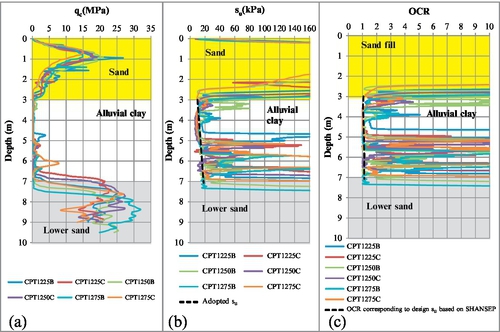
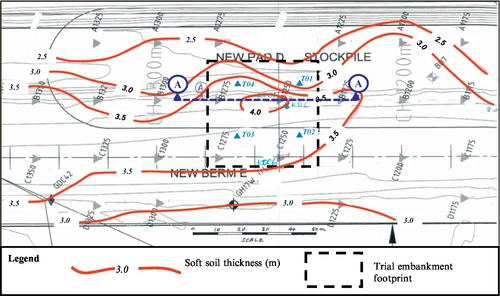
Figure 18.16(b) shows that for the soft clay layer, the inferred representative undrained shear strength, su increases from about 11 to 20 kPa at depths of 3–7 m. These su values were derived using a cone-bearing factor, Nk of 15, which was calibrated against the corrected in situ vane shear data.
The overconsolidation ratio, OCR profiles shown in Fig. 18.16(c) indicate that the soft clay layer is close to its normally consolidated state, with the assessed in situ OCR values being equal to or close to 1. These OCR values were inferred from the su profiles based on the relationship proposed by Ladd (1991):
where σ′vo is the initial effective stress. For sedimentary clays of low to moderate sensitivity with plasticity index PI of 20–80%, Ladd (1991) has adopted the following relationships:
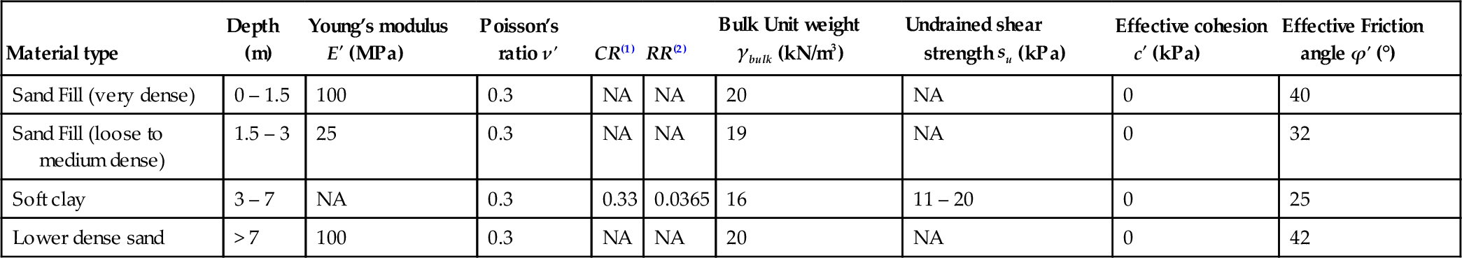
For an averaged PI value of 0.54, as shown in Fig. 18.14(d), S is assessed to be about 0.227. Also, using an averaged RR/CR ratio (= cr/cc) of 0.11, as indicated in Fig. 18.15(c), m is calculated to be about 0.8. Table 18.2 presents the geotechnical model that was developed at the deepest soft soil location within the footprint of the trial pad.
Table 18.2
Geotechnical model and adopted soil parameters
| Material type | Depth (m) | Young’s modulus E′ (MPa) | Poisson’s ratio ν′ | CR(1) | RR(2) | Bulk Unit weight γbulk (kN/m3) | Undrained shear strength su (kPa) | Effective cohesion c′ (kPa) | Effective Friction angle ϕ′ (°) |
| Sand Fill (very dense) | 0 – 1.5 | 100 | 0.3 | NA | NA | 20 | NA | 0 | 40 |
| Sand Fill (loose to medium dense) | 1.5 – 3 | 25 | 0.3 | NA | NA | 19 | NA | 0 | 32 |
| Soft clay | 3 – 7 | NA | 0.3 | 0.33 | 0.0365 | 16 | 11 – 20 | 0 | 25 |
| Lower dense sand | > 7 | 100 | 0.3 | NA | NA | 20 | NA | 0 | 42 |
Notes to Table 18.2:
(1) CR = compression ratio = cc/(1 + eo), where cc is the compression index and eo is the initial void ratio.
(2) RR = recompression ratio = cr/(1 + eo), where cr is the recompression index and eo is the initial void ratio
18.6.3 Stone columns
Stone columns were installed as a ground improvement scheme below the coal pad and berm. The stone columns were installed using the vibro-replacement technique with a top feed wet installation method. Such a technique introduces a coarse-grained material as load-bearing elements consisting of gravel or crushed stone aggregate as a backfill medium. The spacing of the columns in the trial pad area was in a square configuration with 2.75 m center-to-center spacing. The column diameter varied with depth as discussed in the “Stone column diameter” section that follows. The selection of design friction angle of the stone columns is outlined in the “Friction angle of stone columns” section.
Stone column diameter
During the installation of the stone columns, the oscillating vibrator with its extension tubes sunk rapidly into the soil under its own weight with the assistance of water jetting. Aggregates were then imported using a loader and deposited around the probe point to fall into the annular space. The vibrator is slowly withdrawn in short steps and the stone falls to the tip of the vibrator. The vibrator is then lowered back into the hole between 0.7 and 0.8 m and densifies the aggregates using vibration, thereby creating progressive stepped length of densified stone column.
The action of the vibrator compresses stone radially into the surrounding soil and also compacts the stone in the annular space, resulting in a stone column of a diameter that is dependent on the relative stiffness of the in situ soil. A larger diameter is achieved in the soft clays compared to the dense sand fill for a given energy/amperage drawn. The as-constructed column diameters were 1.2 m in the soft clay layer and between 0.6 and 1.1 m in the sand fill layer.
Friction angle of stone columns
The friction angle of granular soil is not a material constant, but depends on relative density and pressure level. It has been shown by de Beer (1965) that the friction angle of sand decreases with increasing confining pressure, thus implying a curved soil failure envelope. Bolton (1986) related this nonlinear strength behavior of sand to the dilatant characteristics described by the well-known stress-dilatancy theory, and related the peak friction angle ϕ′peak for a given granular soil with the soil relative density Dr, the mean effective stress p′, and the critical state friction angle ϕ′crit.
Extensive experimental work has been done in relation to the strength properties of granular soils that are relevant to stone column design. Tests on round Hochstetten gravel by Herle (1997) yielded a residual friction angle of 36° and calculated peak friction angles depending on the relative density Dr, as follows:
• ϕ′ peak = 45° at Dr = 70%
• ϕ′ peak = 50° at Dr = 80%
• ϕ′ peak = 60° at Dr = 90%
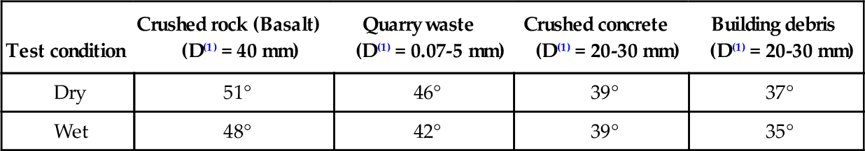
Moroto and Ishii (1990) carried out triaxial compression tests on two rounded natural river gravels and five angular crushed gravels under a cell pressure level of up to 200 kPa. The test results indicated that the friction angles for the rounded and angular gravels are 45–46° and 43– 48°, respectively. The average value for both types of gravels was of the same order, but the void ratio for rounded gravels is smaller (i.e. higher in density). McKelvey et al. (2002) has carried out large shear tests on different materials intended for use in stone columns. Their test results are summarized in Table 18.3.
Table 18.3
Angle of internal friction of various construction materials for vibro stone columns (cited McKelvey et al., 2002)
| Test condition | Crushed rock (Basalt) (D(1) = 40 mm) | Quarry waste (D(1) = 0.07-5 mm) | Crushed concrete (D(1) = 20-30 mm) | Building debris (D(1) = 20-30 mm) |
| Dry | 51° | 46° | 39° | 37° |
| Wet | 48° | 42° | 39° | 35° |
Note to Table 18.3:
(1) D = particle size.
For the present Kooragang ground treatment work, the materials used for the stone column installation are gravels/crushed rocks. The recorded angle of repose from the stockpile prior to installation was 42°, which is considered as a lower bound friction angle for design. The adopted peak friction angle for the present numerical work, based on published data, consideration of the measured angle of repose, and review of the installation method, was 46°.
18.6.4 Full-scale trial pad
A large-scale trial pad load test was performed on working columns in the region of the deepest soft clay zone. The trial pad was about 5.0 m high with a crest plan area of about 20 m × 20 m. To further simulate the working conditions, additional load was imparted by the use of sand-filled shipping containers placed on top of the embankment to provide a total surcharge load of about 40 kPa (under the containers). Following a trial load monitoring for a period of about two months, the pad and the containers were removed.
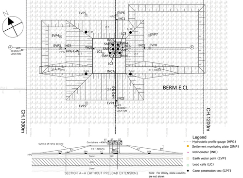
A suite of borehole inclinometers, settlement monitoring plates, hydrostatic profile gauges (HPG), survey vector points, and load cells was installed for the monitoring of the performance of the trial pad, as shown in Fig. 18.18.
18.6.5 Prediction of the trial pad load test using two-dimensional finite element analysis with an equivalent strip method
The modeling of the trial pad load test over stone-column-treated soft ground was carried out by 2D FEA with equivalent strips using PLAXIS software. A section following the HPG in the east–west direction (i.e., section A-A shown in Figs. 18.17 and 18.18) was adopted for the numerical analysis. The 2D FEA model included the upper sand fill, soft clay unit, and lower sand horizon extended to a depth of 30 m below the natural ground surface. The variable soft clay thickness, as depicted on the soft clay thickness isopachs shown in Fig. 18.17, was simulated by varying the base level of the soft clay unit. The soft clay thickness in the back-analysis model varied between about 3.2 m and 4.2 m. The geometry of the FEA model is shown in Fig. 18.19.

The soft clay layer in the 2D FEA was modeled using “Soft Soil Model” in PLAXIS, which resembles the modified Cam-clay model but with a Mohr–Coulomb hexagon yield surface in the deviatoric plane. Conversely, the sand fill and the lower dense sand were modeled using Mohr–Coulomb model. The adopted soft soil model parameters are given in Table 18.2. Note that the modified compression index λ* and the modified swelling index κ* used in PLAXIS can be obtained from the measured laboratory CR and RR values based on λ* = CR/2.3 and κ* = 2RR/2.3, respectively.
The stone columns were modeled as equivalent strips that are represented by Mohr–Coulomb materials with an adopted Poisson ratio of 0.3, which was taken to be the value for the soil itself. The width and the spacing of the equivalent strips were in accordance with that outlined in Fig. 18.1. The equivalent Young’s modulus Eeq and cohesion ceq of the strips were calculated based on the weighted average approach as given in Eq. (18.1). The equivalent friction angle ϕeq was calculated based on Eq. (18.2). For the stone columns founded on the lower dense sand that is considered to be a rigid base, the stress concentration ratio, n in Eq. (18.2), was assessed using the design chart as given in Fig. 18.4. The calculated design parameters of the equivalent strip in the different soil layers are summarized in Table 18.5.
Table 18.5
Design parameters for equivalent strips
| Depth below existing ground z (m) | Soil layer | Soil friction angle ϕ′soil (degrees) | Soil Young’s modulus E′soil (MPa) | Stress concentration ratio, n | ϕ′eq for equivalent strip in 2D FEA (degrees) | E′eq for equivalent strip in 2D FEA(4) (MPa) | |
| 0 – 1.5 | Very dense sand | 40 | 100 | 0.1(2) | 1 | 42.2 | 100 |
| 1.5 – 3 | Loose to medium dense sand | 32 | 25 | 0.3(2) | 3 | 41.2 | 51 |
| 3 – 5 | Soft clay | 25 | 1.8(1) | 0.5(2) | 5(3) | 41.6 | 36 |
| 5 – 7 | Soft Clay | 25 | 2.2(1) | 0.75(2) | 5.5(3) | 41.9 | 36 |
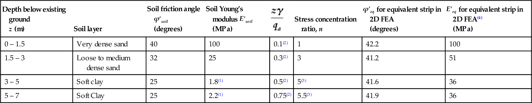
Notes to Table 18.5:
(1) In the 2D FEA, Soft Soil Model was used to model the soft clay, in which the soil compressibility was calculated based on λ* and κ*. For the derivation of equivalent strip parameter, however, E′ is required and has been assessed based on E′ = 150 × su.
(2) z is the depth to the middle of the layer. qa = 140kPa calculated based on 5 m of fill + 40kPa container load.
(3) The strips are divided into several segments, each of which has different strength properties that correspond to the varying stress concentration ratio, n along the column depth as determined from Figure 18.4.
(4) Calculated in conjunction with the adopted Young’s Modulus of stone column, Ecolumn, of 100 MPa.
The trial pad was modeled as a separate material using the Mohr–Coulomb model while the containers were simulated using a 40 kPa surcharge load over the container area. Furthermore, based on the survey vector peg readings and advice from site personnel, a “bridging sand” layer above the upper sand fill unit was added to the model to take into account ground-leveling work and some heaving of the ground surface due to the installation of the stone columns. The bridging sand layer was about 0.6 m thick on the western side of the trial pad and 1.1 m on the eastern side of the trial pad.
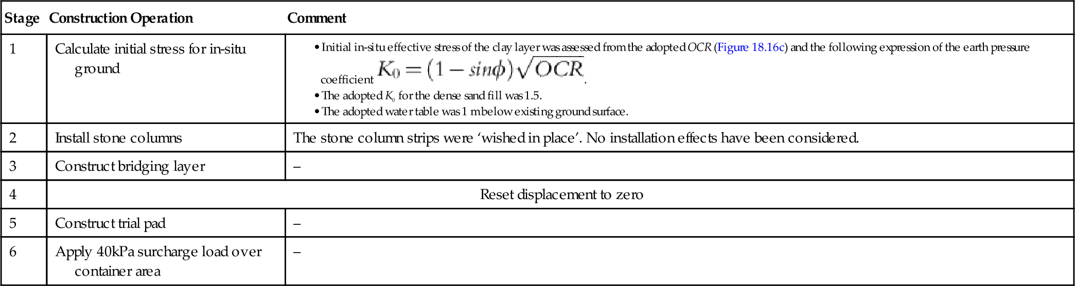
Table 18.4 summarizes the construction sequence adopted in the numerical analysis. Note that the 2D FEA undertaken was an elastoplastic analysis for the assessment of long-term deformation in which the decay of excess pore pressure with time during the primary consolidation stage was not taken into account.
Table 18.4
Adopted construction sequences in the 2D FEA
| Stage | Construction Operation | Comment |
| 1 | Calculate initial stress for in-situ ground |
• Initial in-situ effective stress of the clay layer was assessed from the adopted OCR (Figure 18.16c) and the following expression of the earth pressure coefficient • The adopted K0 for the dense sand fill was 1.5. • The adopted water table was 1 m below existing ground surface. |
| 2 | Install stone columns | The stone column strips were ‘wished in place’. No installation effects have been considered. |
| 3 | Construct bridging layer | ‒ |
| 4 | Reset displacement to zero | |
| 5 | Construct trial pad | ‒ |
| 6 | Apply 40kPa surcharge load over container area | ‒ |
18.6.6 Modeling results and measurements
Settlement
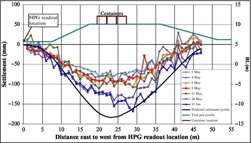
Vertical settlement of the ground surface underneath the trial embankment was regularly monitored at the HPG locations. Figure 18.20 indicates that after the completion of loading, the rate of settlement as recorded by the HPG along section A-A has reduced to a stable small value within one month after the fill placement and the application of the container load. The predicted maximum settlement was 180 mm, which is consistent with the monitored value of 170 mm. The predicted settlement profile is reasonably consistent with the measured HPG profile. However, the position of the predicted maximum settlement occurred directly under the heavy container area, while the measured maximum value was slightly offset by some 5 m. It is considered that this slight offset was possibly due to instrument inaccuracy and inevitable local variation of material properties.
Horizontal soil displacement
Horizontal displacement of the subsoils at the toes of the trial pad was measured at inclinometers INC4 (west) and INC2 (east). Figure 18.21(a) shows that the predicted horizontal profile on the western side compares reasonably well with the INC4 monitored results with regards to the horizontal displacement at the ground surface (≤ 3 mm), as well as the maximum displacement within the clay layer (about 23 mm)
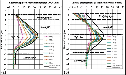
For the eastern side of the trial pad, the predicted horizontal profile within the upper sand fill differs slightly from the measured INC2 monitored results (Fig. 18.21(b)). A closer review of the inclinometer measurements indicated that the first set of monitoring results was likely to be erroneous. It is thus likely that some problems occurred during the installation of this inclinometer, or the datum readings of INC2 were taken prior to the inclinometer casing was fully stabilized, thus affecting the relative displacements since the datum readings were taken. Nevertheless, it is noted that both the measured and predicted movements are minimal, bearing in mind the size of the surcharge and embankment. As such, while relatively large in percentage, the absolute values of horizontal ground surface displacement were minimal and fell within the same order of magnitude as the prediction.
Vertical stress
Three load cells were installed at the ground surface prior to the construction of the trial pad. Two load cells were located underneath the heavy container area: one (LC3) directly on top of a stone column, while the other one (LC2) in-between the columns. The third load cell (LC1) was placed at some 3 m from the containers on top of another stone column. The vertical pressures recorded by the load cells were 152 kPa, 111 kPa, and 132 kPa, respectively. These results are somewhat unexpected since the maximum pressure recorded at LC1 was located away from the heavy container area.
Figure 18.22 shows the predicted profiles of the increased vertical effective stress, both at the top of the bridging layer over the stone columns at approximately RL5.5 m (section X-X) and along a section within the soft clay unit at RL0.0 m (section Y-Y). It can be seen from section Y-Y within the clay unit that the majority of the imparted load was carried by the stone columns.
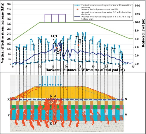
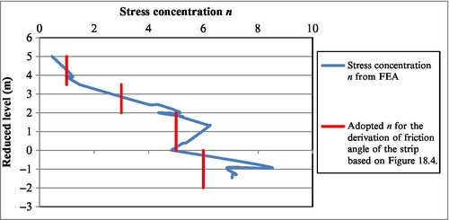
At the area underneath the containers where axisymmetric loading condition is prominent, the ratio of the predicted averaged stress increase within the column strip at section J-J to the stress increase within the surrounding soil at section K-K is plotted in Fig. 18.23. It can be seen that the stress concentration ratio n obtained from the FEA is commensurate with that assessed from Fig. 18.4. (Refer to Table 18.5 for the adopted stress concentration ratio, n, in the derivation of the friction angle of the equivalent strip.) Away from the containers and toward the areas underneath the fill batter, the columns tend to carry a higher proportion of load and therefore higher stress concentration, as the yielding zones within the columns reduce.
For the section at the top of the bridging layer (section X-X), the vertical effective stress distribution between the stone columns and the upper sand fill is significantly less dramatic with the vertical stress varying between 80 kPa and 160 kPa over the entire trial pad top area. The variation is in reasonably good agreement with the measured load cell results, as shown in Fig. 18.22.
18.7 Conclusion
A 2D finite element approach for analyzing the response of stone columns under embankment loading was presented. One of the key features in the 2D FEA is the modeling of the stone columns as equivalent strips that account for, in a 3D sense, the load transfer mechanism between stone columns and the surrounding soils. The equivalent cohesion and Young’s modulus of the strips can be calculated based on a weighted average approach, whereas the equivalent friction angle can be derived based on a force equilibrium method, which requires a presumption of the stress concentration ratio of the stone columns (defined as the ratio of vertical stress within the stone column to the vertical stress of the surrounding soil).
For convenience, charts to assess the stress concentration ratio were generated for full depth and floating stone columns. The chart solutions cover key parameters including (1) load levels, (2) ratio of unit cell diameter to column diameter, de/dc, (3) Ecolumn/Esoil ratio, (4) Ebase/Ecolumn ratio, (5) Ebase/Esoil ratio, and (6) friction angle of stone columns ϕ column.
The accuracy of the proposed 2D FE strip model was investigated by comparing the results with the baseline solutions obtained from the full 3D and axisymmetric FEA. The results indicated that the 2D strip model is able to capture the “bulging” mechanism of the stone columns under an axially symmetric loading condition away from the embankment fill batter, and the “bulging” and “leaning” deformation toward the fill batter. The predictions of vertical and horizontal displacements at various positions across the embankment agreed reasonably well with baseline solutions.
Conversely, the 2D FE model using conventional composite block material is unable to capture the bulging and leaning of the stone columns. The solution grossly underpredicts the vertical and horizontal displacements near the embankment batter when compared with the baseline solutions, although it gives a comparable vertical displacement result under an axially symmetric loading condition. Thus the 2D strip FE model is preferable over the 2D block model for stone column design, particularly when horizontal displacement or edge deformation is critical.
To validate the design approach, survey measurements from a large-scale area load test over working stone columns was used to compare with the numerical predictions using the proposed 2D FE strip method. The 5-m-high trial embankment was built over an area of 40 m2. To further simulate the working conditions, additional load was imparted by the use of sand-filled shipping containers placed on top of the embankment. The test was instrumented and monitored, including settlement plates, hydrostatic profile gauge, load cells, inclinometers, and survey monuments.
In summary, the FE modeling results predicted maximum test pad settlement and maximum horizontal displacement of some 180 mm and 23 mm, respectively, for the “as constructed” case. These predictions compare with the measured maximum values of 170 mm and 24 mm. Similarly, the FE predictions of the vertical stresses below the containers, at the original ground surface level, are about 155 kPa and 110 kPa at the columns and in-between columns, respectively. These values again compare (favorably) with the corresponding measured results of 152 kPa and 111 kPa. The actual monitoring results were thus considered to be in reasonably good agreement with (but slightly lower than) the predicted results.