
9
The Counterfactual Explanations Method
The EU General Data Protection Regulation (GDPR) states that an automatic process acting on personal data must be explained. Chapter 2, White Box XAI for AI Bias and Ethics, described the legal obligations that artificial intelligence (AI) faces. If a plaintiff requires an explanation for a decision that a machine learning (ML) application made, the editor of the AI system must justify its output.
In the previous chapters, we used a bottom-to-top method to understand an explainable AI (XAI) method. We displayed the source code. We then saw how the data was loaded, vectorized, preprocessed, and split into the training/test datasets. We described the mathematical representation of some of the ML and deep learning algorithms in the programs. We also defined the parameters of the ML models.
In Chapter 4, Microsoft Azure Machine Learning Model Interpretability with SHAP, we calculated the Shapley value of a feature to determine its marginal contribution to a positive or negative prediction.
In Chapter 8, Local Interpretable Model-Agnostic Explanations (LIME), we scanned the vicinity of an instance to explain a prediction locally.
Counterfactual explanations look at AI from another perspective. In a real-life situation, an editor who may have invested considerable resources in an AI system does not want to make it public. The legal obligation to explain an ML process in detail can become a threat to the very survival of the editor's business. Yet an explanation must be provided.
The counterfactual explanation approach introduces a new dimension: unconditionality. Unconditional explanations take us a step further. We will go beyond positive and negative predictions. We will look at a result irrespective of whether or not it was fully automated.
Counterfactual explanations do not require opening and looking inside a "black box" algorithm, the preprocessing phases, and whether they were automated. We do not need to understand the algorithm, read its code, or even know what the model does at all.
Counterfactual explanations require a new challenging approach for an AI specialist, a top-to-bottom approach.
In this chapter, we will begin to view counterfactual explanations through distances between two predictions and examine their features. We will have a user's perspective when objectively stating the position of two features regardless of their classification or origin (automated or semi-automated).
We will then leave the top layer of the counterfactual explanation, moving to explore the logic and metrics of counterfactual explanations.
Finally, we will then reach the code level and describe the architecture of this deep learning model.
This chapter covers the following topics:
- Visualizing counterfactual distances in the What-If Tool (WIT)
- Running
Counterfactual_Explanations.ipynbin Google Colaboratory - Defining conditional XAI
- Defining belief in a prediction
- Defining the truth of a prediction
- Defining justification
- Defining sensitivity
- L1 norm distance functions
- L2 norm distance functions
- Custom distance functions
- How to invoke the What-If Tool
- Custom predictions for WIT
- XAI as the future of AI
Our first step will be to explore the counterfactual explanations method with examples.
The counterfactual explanations method
In this chapter and section, we will be exploring AI explanations in a unique way. We will not go through the "getting started" developer approach and then explore the code in sequential steps from beginning to end.
We will start from a user's perspective when faced with factual and counterfactual data that require an immediate explanation.
Let's now see which dataset we are exploring and why.
Dataset and motivations
Sentiment analysis is one of the key aspects of AI. Bots analyze our photos on social media to find out who we are. Social media platforms scan our photos daily to find out who we are. Our photos enter the large data structures of Google, Facebook, Instagram, and other data-collecting giants.
Smiling or not on a photo makes a big difference in sentiment analysis. Bots make inferences on this.
For example, if a bot detects 100 photos of people, which contain 0 smiles and 50 frowns, that means something. If a bot detects 100 pictures of a person with 95 smiles, this will mean something else.
A chatbot with a connected webcam will react according to facial expressions. If a person is smiling, the chatbot will be chirpy. If not, the chatbot might begin the conversation with careful small talk.
In this chapter, we will be exploring the CelebA dataset, which contains more than 200,000 celebrity images with 40 annotated attributions each. This dataset can be used for all types of computer vision tasks, such as face recognition or smile detection.
This chapter focuses on counterfactual data points for smile detection.
We will now visualize counterfactual distances in WIT.
Visualizing counterfactual distances in WIT
Open Counterfactual_Explanations.ipynb in Google Colaboratory. The notebook is an excellent Google WIT tutorial to base counterfactual explanations on. In this section, we will use WIT's counterfactual interface as an AI expert who demands an explanation for certain results produced by an AI system.
The WIT widget is installed automatically at the start of the program.
The program first automatically imports tensorflow and prints the version:
import tensorflow as tf
print(tf.__version__)
You will be asked to restart the notebook. Restart the program (from the Runtime menu) and then click on Run all.
Then, automatically install the widget:
# @title Install the What-If Tool widget if running in Colab
# {display-mode: "form"}
!pip install witwidget
We will not be running the program cell by cell in this top-to-bottom approach. We will run the whole program and start analyzing the results interactively. To do so, open Runtime in the menu bar and click on Run all:

Figure 9.1: Running the program
Once the program has gone through all of the cells, scroll down to the bottom of the notebook until you reach the Invoke What-If Tool for the data and model cell.
You will see a region on the right side of the screen with smiling faces and not-so-smiling faces. To view the images in color, set Color By to (none):

Figure 9.2: Displaying images as data points
On the left side of WIT's interface, you should see an empty screen waiting for you to click on a data point and begin analyzing the data points:

Figure 9.3: The WIT interface
This top-to-bottom process leads us to explore WIT with the default settings going down the interface, level by level.
Exploring data point distances with the default view
The data points are displayed by their prediction value. Choose Inference value in the Label By drop-down list:

Figure 9.4: Choosing a label name
The data point labels appear with their prediction value:

Figure 9.5: Inference values of the data points
Now, set Label By to (none) and Color By to Inference value. This time, the images will appear again with one color for images classified as smiling (top images) and another for the not smiling (bottom) images. The higher the image, the higher the probability the person is smiling:

Figure 9.6: Displaying the data points by the color of the prediction value
To begin a counterfactual investigation, click on one of the images:

Figure 9.7: Selecting a data point
The features of the data point will appear on the left side of the interface:

Figure 9.8: Attributes of the data point
Scroll down under the image to see more features. Now activate the Nearest counterfactual data point function:

Figure 9.9: Activating the Nearest counterfactual function
We now see the counterfactual features of the counterfactual datapoint next to the data point we selected. The closest counterfactual data point is a person classified as "smiling":

Figure 9.10: Visualizing the data point and its counterfactual data point
We now see the attributes of the image of the "smiling" person on the left side of the interface:
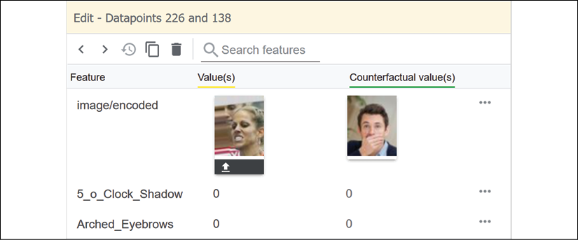
Figure 9.11: Comparing the attributes of two data points
A human can easily see that there is a problem here! We do not really know what these people are doing! Is the person on the left sort of happy and smiling? Who knows what the person on the right is doing?
If we scroll down to compare the features of both images, we can see that both images are labeled as not smiling:

Figure 9.12: Two possible features of an image
This raises several issues on the reliability of the model. First, we can imagine some issues from a counterfactual explanations' unconditional perspective for the person of the left:
- This picture does not really prove the person is smiling or not smiling.
- This person could have this sort of expression when expressing a happy, "Yes, I did it!" moment.
- Why choose such a picture to illustrate that a person is smiling or not?
- How can a mouth covered by a hand end up in the Smiling category?
Maybe we are wrong and are not interpreting the image correctly. You can play around with WIT. That's the whole purpose of the interface.
To check, set Label By to Inference value and Color By to Inference score:

Figure 9.13: Showing the prediction value of a data point and its counterfactual data point
The inference value of the person on the right is clearly 1.
If we apply this to other domains, we see how unconditional counterfactual explanations will provide the legal basis for many lawsuits in the coming years:
- Suppose 1 represents a person who obtained a loan from a bank, and 0 represents a person who did not obtain the same type of loan. It is impossible to know if the positive prediction can be verified or not. The prediction was made without sufficient information. The person who did not get the loan will undoubtedly win a damage suit and also win punitive damages as well.
- Suppose 1 represents a cancer diagnosis and 0 a clean health diagnosis although they have similar attributes.
Imagine as many other similar situations as you can before continuing this chapter using an unconditional counterfactual explanation approach.
We can now sum up this first top level:
- Unconditional: We are not concerned about where this data comes from or about the AI model used. We want to know why one person "obtains" a "smile" (it could be anything else) and why another one doesn't. In this case, the explanation is far from convincing for the AI model involved. Of course, the whole point of this notebook is to show that accurate AI training performances cannot be trusted without XAI.
- Counterfactual: We take a data point at random. We choose a counterfactual point. We decide whether the counterfactual point is legitimate or not.
In a court of law, the AI model proposed here would be in serious trouble. However, the notebook was designed precisely to help us understand the importance of the unconditional counterfactual explanations' method.
XAI has gone from being a cool way to explain AI to a legal obligation with significant consequences, as stated by the GDPR:
"(71) The data subject should have the right not to be subject to a decision, which may include a measure, evaluating personal aspects relating to him or her which is based solely on automated processing and which produces legal effects concerning him or her or similarly significantly affects him or her, such as automatic refusal of an online credit application or e-recruiting practices without any human intervention.
.../...
In any case, such processing should be subject to suitable safeguards, which should include specific information to the data subject and the right to obtain human intervention, to express his or her point of view, to obtain an explanation of the decision reached after such assessment and to challenge the decision."
Regulation 2016/679, GDPR, recital 71, 2016 O.J. (L 119) 14 (EU)
Counterfactual explanations meet these legal requirements.
We will now go to a lower level. We need to go deeper into the logic of counterfactual explanations.
The logic of counterfactual explanations
In this section, we will first go through the logic of counterfactual explanations and define the key aspects of the method.
Counterfactual explanations can first be defined through three key traditional concepts and a fourth concept added by ML theory:
- Belief
- Truth
- Justification
- Sensitivity
Let's begin with belief.
Belief
If we do not believe a prediction, it will shake the foundations of the AI system we are using.
Belief is a bond of trust between a subject S and a proposition p. Belief does not require truth or justification. It can be stated as follows:
If p is believable, S believes p.
A subject S requires no information other than belief to conclude that p is true.
For example, S, based on human experience, can believe four assertions based on the following image:
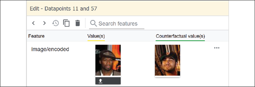
Figure 9.14: Comparing the images
- p is true: The person on the left is not smiling.
- p is true: The statement that the person on the left is smiling is false.
- p is true: The person on the right is smiling.
- p is true: The statement that the person on the right is not smiling is false.
If an AI system makes these assertions, S will believe them.
However, in the following case, S's belief in the AI system might be shaken.
The following screenshot is difficult to believe. The inference score of the person on the left is 0 (not smiling), and the inference score of the person on the right is 1 (smiling):

Figure 9.15: A false negative and a true positive
In this case, the issue shakes S's belief:
If p is false, S cannot believe p.
This assertion can rapidly lead to more doubts:
If this p is false, S cannot believe any other p.
The counterfactual distances between the two people contribute to a lack of belief in the AI system's ability to predict:

Figure 9.16: Visualizing the distance between two data points
The distance between the two smiling people goes beyond S's belief in the system.
We will now see the contribution of truth when analyzing counterfactual explanations.
Truth
Suppose S, the subject observing an AI system, believes p, the assertion made by the system.
Even if S believes p, p must be true, leading to the following possibilities:
- S believes p; p is false.
- S believes p; p is true.
When applying counterfactual XAI methods, the following best practice rules apply:
- Without belief, S will not trust an apparent truth.
- Belief does not imply truth.
Take a moment to observe the following screenshot:
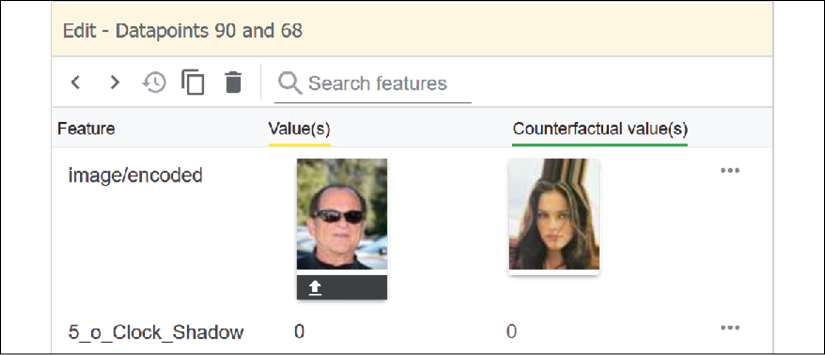
Figure 9.17: Detecting whether or not a person is smiling
The notebook's model makes the following assertions:
p: The person on the left is smiling, and the person on the right is not smiling.
In this situation, S believes p, however, is p true?
If you looked closely at the image of the person on the left, the person could be smiling or could be blinded by sunlight, squinting, and tightening his face.
However, the prediction score for this image is 1 (true, the person is smiling).
At this point, the counterfactual explanation situation can be summed up as follows:
S believes p.
p can be the truth.
However, p must now be justified.
Justification
If an AI system fails to provide sufficient explanations, we could refer to the good practice required by GDPR:
"In any case, such processing should be subject to suitable safeguards, which should include specific information to the data subject and the right to obtain human intervention, to express his or her point of view, to obtain an explanation of the decision reached after such assessment and to challenge the decision."
Regulation 2016/679, GDPR, recital 71, 2016 O.J. (L 119) 14 (EU)
If a company has the resources to have a hotline that can meet the number of justifications required, then the problem is solved as follows:
S believes p; p might be true; S can obtain justification from a human.
This will work if:
- The number of requests is lower than the capacity of the hotline to answer them.
- The hotline has the capacity to train and make AI experts available.
As AI expands, a better approach would be to:
- Implement XAI as much as possible to avoid consuming human resources.
- Make human support available only when necessary.
In this section, we saw that justifications make an explanation clearer for the users.
We will now add sensitivity to our counterfactual explanation method.
Sensitivity
Sensitivity is an essential concept for counterfactual explanations. It will take the explanations to the core of the method.
In the Belief section, belief could be compromised; see the following:
If p is false, S cannot believe p.
This assertion can rapidly lead to more doubts:
If this p is false, S cannot believe any other p.
This negative assertion does not solve the problem. Not believing in p only expresses doubt, not the truth, and doesn't provide any justification. Truth can determine whether or not p is true. Justification can provide interesting rules. Sensitivity will bring us closer to the explanation we are looking for.
Let p be a false negative prediction for a person who was, in fact, smiling but was classified as not smiling.
Let Xtp be the data points in the dataset that are true positives of people who are smiling:
Xtp = {x1, x2, x3, ..., xn,}
Our goal will be to find data points that have a set of features that are the closest to p, such as in the following example:

Figure 9.18: Visualizing sensitivity
In this section, we went through the key concepts of counterfactual explanations: belief, trust, justification, and sensitivity.
We will now select the best distance functions for counterfactual explanations.
The choice of distance functions
WIT uses a distance function for its visual representation of data points.
If you click on the information symbol (i) next to Nearest counterfactual, WIT shows the three distance function options available:

Figure 9.19: Choosing a distance function
In this section, we will go through these options, starting with the L1 norm:
- The L1 norm
- The L2 norm
- Custom distance
The L1 norm
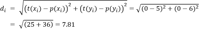
The L1 norm is the Manhattan or taxicab norm because it calculates distances in a way that resembles the blocks in Manhattan. The following diagram shows a grid like the blocks of buildings in Manhattan, New York City:

Figure 9.20: Manhattan distance
Suppose you take a cab at point [0, 0] and want to go to point [5, 6]. The driver will go 5 blocks in a straight line (see the blocks in gray) and will then turn to the left and drive 6 blocks (see the path in gray). You will pay a distance of 5 + 6 blocks = 11 blocks, represented as follows:
Distance to pay = 5 blocks + 6 blocks = 11 blocks
If we now translate this expression into a mathematical expression of the L1 norm, we obtain the following:
![]() , or in this case,
, or in this case, ![]()
This value is the distance for one data point.
We can also translate our taxicab expression in the least deviations function. The variables are:
- Yi: The target values
- p(Xi): The predicted values produced by the ML model
- S: The sum of the absolute differences between the target values and the predicted values
Yi can be compared to the shortest way for the taxicab driver to get to the point we want to get to.
p(Xi) can be compared to a cab driver who does not take the shortest path to the point we want to go to and takes us a longer way. This could be the cab driver's first day on the job with a GPS system that is not working.
S is the absolute difference between the distance we wanted to pay, the shortest one, and the longer distance the cab took.
The mathematical expression to measure all of the n paths a cab took in one day for all customers, for example, is as follows:

There are variations of L1 in which you can divide the sum of the values by other statistical values. A simple variation is to divide the result by the number n of cab fares in the day, in our example, to obtain a mean deviation for this cab driver.
At the end of the day, we might find the mean deviation of this cab driver is the total deviations/number of fares = mean deviation. This is only one variation.
In any case, the goal in ML is to minimize the value of L1 to improve the accuracy of a model.
This explanation captures the essence of L1, a robust and reliable distance function.
The L2 norm is also widely used as a distance function.
The L2 norm
The L2 norm calculates the shortest path between two points. Unlike the Manhattan method, it can go straight through the buildings. Imagine the L2 norm as "a bird's distance" from one point to another:

Figure 9.21: Euclidean distance
L2 uses the Euclidean distance between two points.
yi represents the t(x) and t(y) coordinates of the target prediction and p(xi) represents the p(x) and p(y) coordinates of a prediction.
The Euclidean distance can be expressed as follows:

In our taxicab case, t(x) = 0 and t(y) = 0 at the point of origin. The Euclidean distance is as follows:
The goal in ML is, as for L1, to minimize the value of L2 to improve the accuracy of a model.
We can also use a custom distance function for WIT.
Custom distance functions
WIT's custom function for this image dataset uses numpy.linalg.norm, which provides a range of parameters and options, more information about which can be found at https://docs.scipy.org/doc/numpy/reference/generated/numpy.linalg.norm.html.
In this case, we can see that the distance function calculates the current distance to the average color of the images:
# Define the custom distance function that compares the
# average color of images
def image_mean_distance(ex, exs, params):
  selected_im = decode_image(ex)
  mean_color = np.mean(selected_im, axis=(0, 1))
  image_distances = [np.linalg.norm(mean_color –
    np.mean(decode_image(e), axis=(0, 1))) for e in exs]
  return image_distances
We have gone through the counterfactual explanations' method and distance functions. We will now drill down into the architecture of the deep learning model.
The architecture of the deep learning model
In this section, we will continue the top-to-bottom, user-oriented approach. This drill-down method takes us from the top layer of a program down to the bottom layer. It is essential to learn how to perceive an application from different perspectives.
We will go from the user's point of view back to the beginning of the process in the following order:
- Invoking WIT
- The custom prediction function for WIT
We will first see how the visualization tool is launched.
Invoking WIT
You can choose the number of data points and the tool's height in the form just above WIT as shown in the following screenshot:

Figure 9.22: WIT parameters
The form is driven by the following code:
# Decode an image from tf.example bytestring
def decode_image(ex):
  im_bytes = ex.features.feature['image/encoded'].bytes_list.value[0]
  im = Image.open(BytesIO(im_bytes))
  return im
We already explored the custom distance function in The choice of distance functions section:
# Define the custom distance function that compares
# the average color of images
The program now sets the tool up with WitConfigBuilder, with num_datapoints defined in the form just above the cell, and the custom image_mean_distance function described in the custom distance function in The choice of distance functions section:
# Setup the tool with the test examples and the trained classifier
config_builder = WitConfigBuilder(
    examples[:num_datapoints]).set_custom_predict_fn(
        custom_predict).set_custom_distance_fn(image_mean_distance)
WitWidget now displays WIT, taking the height defined in the form above the cell into account:
wv = WitWidget(config_builder, height=tool_height_in_px)
WIT displays the interface explored in The counterfactual explanations method section.
Note that config_builder calls a custom prediction function for images named custom_predict, which we will now define.
The custom prediction function for WIT
WIT contains a custom prediction function for the image dataset of this notebook. The function extracts the image/encoded field, which is a key feature that contains an encoded byte list. The feature is read into BytesIO and decoded back to an image using Python Imaging Library (PIL).
PIL is used for loading and processing images. PIL can load images and transform them into NumPy arrays. In this case, arrays of images are floats between 0.0 and 1.0. The output is a NumPy array containing n samples and labels:
def custom_predict(examples_to_infer):
  def load_byte_img(im_bytes):
    buf = BytesIO(im_bytes)
    return np.array(Image.open(buf), dtype=np.float64) / 255.
  ims = [load_byte_img(
    ex.features.feature['image/encoded'].bytes_list.value[0])
      for ex in examples_to_infer]
  preds = model1.predict(np.array(ims))
  return preds
You can call this function from the interface. Note that the model, model1, is called in real time. First, click on a data point, then activate the Nearest counterfactual function, which will use the distance function to find the nearest counterfactual:

Figure 9.23: The nearest counterfactual function
The interface will display the factual and counterfactual data points and their attributes:

Figure 9.24: Comparing two data points
You might want to see what happens if you change the value of an attribute of the factual data point. For example, set Arched_Eyebrows to 1 instead of 0. Then click on the Run inference button to activate the prediction function that will update the prediction of this data point:

Figure 9.25: WIT's prediction function
The data point might change positions with a new visible prediction change. Activate Nearest counterfactual to see whether the nearest counterfactual has changed.
Take some time to experiment with changing data point attributes and visualizing the changes.
WIT relies on a trained Keras model to display the initial predictions.
Loading a Keras model
In this section, we will see how to load a Keras model and envision the future of deep learning.
In this notebook, TensorFlow uses tf.keras.models.load_model to load a pretrained model:
# @title Load the Keras models
from tensorflow.keras.models import load_model
model1 = load_model('smile-model.hdf5')
The model was saved in a serialized model file named smile-model.hdf5.
And that's it!
Only a few years ago, a notebook like this would have contained a full deep learning model such as a convolutional neural network (CNN) with its convolutional, pooling, and dense layers, among others.
We need to keep our eyes on the ball if we want to stay in tune with the rapid evolution of AI.
Our tour of counterfactual explanations in this chapter has shown us two key aspects of AI:
- XAI has become mandatory
- AI systems will continue to increase in complexity year on year
These two key aspects of AI lead to significant implications for AI projects:
- Small businesses will not have the resources to develop complex AI models
- Large corporations will be less inclined to invest in AI programs if ready-to-use certified AI and XAI models are available
- Certified cloud platforms will offer AI as a service that will be cost-effective, offering AI and legal XAI per region
- AI as a service will wipe out many bottom-to-top AI projects of teams that want to build everything themselves
- Users will load their data into cloud platform buckets and wait for AutoML to either provide the output of the model or at least provide a model that can be loaded like the one in this section
- These ready-to-use, custom-built models will be delivered with a full range of XAI tools
Cloud platforms will provide users with AI and XAI as a service. In the years to come, AI specialists will master a broad range of AI and XAI tools that they will mostly implement as components and add customized development only when necessary.
We will now retrieve the dataset and model from this perspective.
Retrieving the dataset and model
Let's continue our top-to-bottom exploration with the future of AI in mind.
The remaining cells represent the functions that will be embedded in an AI as a service platform: retrieving the data and the pretrained model.
The data can be retrieved as a CSV file, as follows:
# @title Load the CSV file into a pandas DataFrame and process it
# for WIT
import pandas as pd
data = pd.read_csv('celeba/data_test_subset.csv')
examples = df_to_examples(data,
    images_path='celeba/img_test_subset_resized/')
The pretrained model is downloaded automatically so you can just focus on using XAI:
!curl -L https://storage.googleapis.com/What-If-tool-resources/smile-demo/smile-colab-model.hdf5 -o ./smile-model.hdf5
!curl -L https://storage.googleapis.com/What-If-tool-resources/smile-demo/test_subset.zip -o ./test_subset.zip
!unzip -qq -o test_subset.zip
This section paved the way for the future of AI. XAI will replace trying to explain a black box model. AI models will become components buried in AutoML applications.
XAI will be the white box of an AI architecture.
The last cell of the notebook lists some more exploration ideas. You can also go back and explore Chapter 6, AI Fairness with Google's What-If Tool (WIT), for example, with the counterfactual explanation method in mind.
A whole world of AI innovations remains ahead of us!
Summary
In this chapter, we approached XAI with a top-to-bottom method. We learned that the counterfactual explanations method analyzes the output of a model unconditionally. The explanation goes beyond explaining why a prediction is true or not. The model does not come into account either. The counterfactual explanations method is based on four key pillars: belief, trust, justification, and sensitivity.
A user must first believe a prediction. Belief will build trust in an AI system. However, even if a user believes a prediction, it must be true. A model can produce a high accuracy rate on a well-designed dataset, which shows that it should be true.
The truth alone will not suffice. A court of law might request a well-explained justification of a prediction. A defendant might not agree with the reasons provided by a bank to refuse a loan based on a decision made by an AI system.
Counterfactual explanations will provide a unique dimension: sensitivity. The method will find the nearest counterfactual data point, which will display the distance between the two data points. The features of each data point will show whether or not the model's prediction is justified. If a loan is refused to one person with an income of x units of currency, but granted to a person with an income of x + 0.1%, we could conclude that the bank's thresholds are arbitrary.
We saw that good practice should lead to working on counterfactual explanations before the model is released to market. A rule base could represent some best-practice rules that would limit the number of errors.
Finally, we examined the innovative architecture of the deep learning model, which minimized the amount of code and resources necessary to implement the AI system.
Counterfactual explanations take us another step forward in the expansion of our understanding of AI, XAI, and AutoML.
In the next chapter, The Contrastive Explanation Method (CEM), we will discover how to identify minimal features that justify a classification.
Questions
- A true positive prediction does not require a justification. (True|False)
- Justification by showing the accuracy of the model will satisfy a user. (True|False)
- A user needs to believe an AI prediction. (True|False)
- A counterfactual explanation is unconditional. (True|False)
- The counterfactual explanation method will vary from one model to another. (True|False)
- A counterfactual data point is found with a distance function. (True|False)
- Sensitivity shows how closely a data point and its counterfactual are related. (True|False)
- The L1 norm uses Manhattan distances. (True|False)
- The L2 norm uses Euclidean distances. (True|False)
- GDPR has made XAI de facto mandatory in the European Union. (True|False)
References
- The reference code for counterfactual explanations can be found at https://colab.research.google.com/github/PAIR-code/What-If-tool/blob/master/WIT_Smile_Detector.ipynb
- The reference document for counterfactual explanations can be found at Counterfactual explanations without opening the black box: Automated decisions and the GDPR. Wachter, S., Mittelstadt, B., and Russell, C. (2017). https://arxiv.org/abs/1711.00399
Further reading
- For more on the CelebA dataset, visit http://mmlab.ie.cuhk.edu.hk/projects/CelebA.html
- For more on GDPR, visit https://eur-lex.europa.eu/legal-content/EN/TXT/PDF/?uri=CELEX:32016R0679