5

Building an Explainable AI Solution from Scratch

In this chapter, we will use the knowledge and tools we acquired in the previous chapters to build an explainable AI (XAI) solution from scratch using Python, TensorFlow, Facets, and Google's What-If Tool (WIT).

We often isolate ourselves from reality when experimenting with machine learning (ML) algorithms. We take the ready-to-use online datasets, use the algorithms suggested by a given cloud AI platform, and display the results as we saw in a tutorial we found on the web. Once it works, we move on to another ML algorithm and continue like this, thinking that we are learning enough to face real-life projects.

However, by only focusing on what we think is the technical aspect, we miss a lot of critical moral, ethical, legal, and advanced technical issues. In this chapter, we will enter the real world of AI with its long list of XAI issues.

Developing AI code in the 2010s relied on knowledge and talent. Developing AI code in the 2020s implies the accountability of XAI for every aspect of an AI project.

In this chapter, we will explore the U.S. census problem provided by Google as an example of how to use its WIT. The WIT functions show the power of XAI. In this chapter, we will approach WIT from a user's point of view, intuitively. In Chapter 6, AI Fairness with Google's What-If Tool (WIT), we will examine WIT from a technical perspective.

We will start by analyzing the type of data in the U.S. census dataset from moral, ethical, legal, and technical perspectives in a pandas DataFrame.

Our investigation of the ethical and legal foundations of the U.S. census dataset will lead us to conclude that some of the columns must be discarded. We must explain why it is illegal in several European countries to use features that might constitute discrimination, for example.

Once the dataset has been transformed into an ethical and legal asset, we will display the data in Facets before using ML to train on the U.S. census dataset. We will go as far as possible, explaining our ethical choices and providing inferences. Finally, we will train on the U.S. census dataset and explain the outputs with WIT.

This chapter covers the following topics:

• Datasets from a moral and ethical perspective
• Datasets from a legal and ML technical perspective
• Learning how to anticipate the outputs of ML through XAI before training the data
• Explaining the expected results with Facets
• Verifying our anticipated results with a k-means clustering algorithm
• Training an ethical dataset with TensorFlow estimators
• XAI with WIT applied to the output of the tested data
• Using WIT to compare the classification of the data points
• AI fairness explained from an ethical perspective

Our first step will be to investigate the U.S. census dataset from moral, ethical, legal, and ML perspectives.

Moral, ethical, and legal perspectives

We will start by examining the U.S. census dataset with the executive function described in Chapter 1, Explaining Artificial Intelligence with Python, as shown in Figure 5.1:

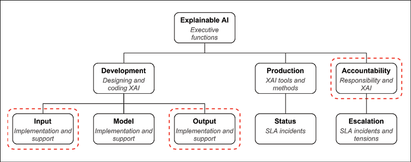
Figure 5.1: Executive function chart

You will notice that we will focus on input, output, and accountability. Developing AI programs comes with moral, ethical, and legal responsibilities. The introduction to Chapter 2, White Box XAI for AI Bias and Ethics, proved that ignoring ethical and legal liabilities can cost millions of any country's currency. Every company, government institution, and individual that uses AI is accountable for the actions taken as a result of the AI algorithms that produce automated outputs.

In this section, we will take accountability seriously by investigating the inputs provided for our program and their impact on the outputs.

Let's examine the U.S. census problem from the different perspectives of accountability.

The U.S. census data problem

The U.S. census data problem uses features of the U.S. population to predict whether a person will earn more than USD 50K or not.

In this chapter, we will use WIT_Model_Comparison_Ethical.ipynb, a notebook derived from Google's notebook.

The initial dataset, adult.data, was extracted from the U.S. Census Bureau database: https://web.archive.org/web/20021205224002/https://www.census.gov/DES/www/welcome.html

Each record contains the features of a person. Several ML programs were designed to predict the income of that person. The goal was to classify the population into groups for those earning more than USD 50K and those earning less.

The adult.names file contains more information on this data and the methods.

The ML program's probabilities, as stated in the adult.names file, achieved the following accuracy:

Class probabilities for adult.all file
| Probability for the label '>50K'  : 23.93% / 24.78% (without unknowns)
| Probability for the label '<=50K' : 76.07% / 75.22% (without unknowns)

We will begin by using pandas to display the data.

Using pandas to display the data

Open the WIT_Model_Comparison_Ethical.ipynb notebook.

We will start by importing the original U.S. census dataset:

# @title The UCI Census data {display-mode: "form"}
import pandas as pd
# Set the path to the CSV containing the dataset to train on.
csv_path = 'https://archive.ics.uci.edu/ml/machine-learning-databases/adult/adult.data'

If you experience problems with this link, copy the link in your browser, download the file locally, and then upload it to Google Colaboratory using the Colab file manager.

We will now define the column names, as described in the original dataset, in the adult.names file:

# Set the column names for the columns in the CSV.
# If the CSV's first line is a header line containing
# the column names, then set this to None.
csv_columns = ["Age", "Workclass", "fnlwgt", "Education",
               "Education-Num", "Marital-Status", "Occupation",
               "Relationship", "Race", "Sex", "Capital-Gain",
               "Capital-Loss", "Hours-per-week", "Country",
               "Over-50K"]

The program now loads the data in a pandas DataFrame and displays it:

# Read the dataset from the provided CSV and
# print out information about it.
df = pd.read_csv(csv_path, names=csv_columns, skipinitialspace=True)
df

The first columns appear as follows:

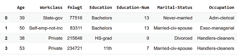
Figure 5.2: Displaying the first columns and lines of the dataset

The following columns are displayed as well:

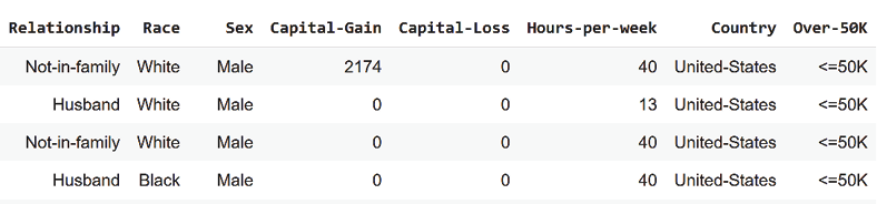
Figure 5.3: Displaying samples of the dataset

adult.names describes the possible contents of each feature column as follows:

age: continuous
workclass: Private, Self-emp-not-inc, Self-emp-inc, Federal-gov, Local-gov, State-gov, Without-pay, Never-worked
fnlwgt: continuous
education: Bachelors, Some-college, 11th, HS-grad, Prof-school, Assoc-acdm, Assoc-voc, 9th, 7th-8th, 12th, Masters, 1st-4th, 10th, Doctorate, 5th-6th, Preschool
education-num: continuous
marital-status: Married-civ-spouse, Divorced, Never-married, Separated, Widowed, Married-spouse-absent, Married-AF-spouse
occupation: Tech-support, Craft-repair, Other-service, Sales, Exec-managerial, Prof-specialty, Handlers-cleaners, Machine-op-inspct,
Adm-clerical, Farming-fishing, Transport-moving, Priv-house-serv, Protective-serv, Armed-Forces
relationship: Wife, Own-child, Husband, Not-in-family, Other-relative, Unmarried
race: White, Asian-Pac-Islander, Amer-Indian-Eskimo, Other, Black
sex: Female, Male
capital-gain: continuous
capital-loss: continuous
hours-per-week: continuous
native-country: United-States, Cambodia, England, Puerto-Rico, Canada, Germany, Outlying-US(Guam-USVI-etc), India, Japan, Greece, South, China, Cuba, Iran, Honduras, Philippines, Italy, Poland, Jamaica, Vietnam, Mexico, Portugal, Ireland, France, Dominican-Republic, Laos, Ecuador, Taiwan, Haiti, Columbia, Hungary, Guatemala, Nicaragua, Scotland, Thailand, Yugoslavia, El-Salvador, Trinadad&Tobago, Peru, Hong, Holand-Netherlands

We now have displayed the data and its content.

Let's conduct a moral experiment like we did in Chapter 2, White Box XAI for AI Bias and Ethics. We will transpose the moral problems from the trolley problem into what we will name the U.S. census data problem. In this case, we are facing the moral dilemma of using sensitive personal information to make a decision.

Imagine you are implementing an AI agent that determines the predicted salary of a given person based on this data. The AI agent is for a company that would like to use cloud-based AI to predict salaries based on U.S. census-type data. Your AI agent has the choice of determining the expected salary of the people in the company of being >50K or <=50K based on the information you are examining. Would you agree to use this type of data to make predictions in a company or on a website?

You have two choices:

• Accept using the dataset as it is. You find a line that fits the person you are predicting the salary for. You apply ML algorithms anyway and predict an income of less or more than 50K. In this case, you might hurt a person's feelings if that person discovers what you did.
• You refuse to use the dataset because it contains information you do not want to use to reach a decision. In this case, you may be fired.

What would you do? Think carefully about this before reading the next section, where we will analyze the U.S. census data problem.

Moral and ethical perspectives

At the end of the last section, your AI agent faces a tough decision on using all of the features in the U.S. census dataset as they are, or not.

You now team up with a few developers, consultants, and a project manager to analyze the potentially biased columns of the dataset.

After some discussion, your team comes up with the following columns that require moral and ethical analysis:

Workclass	Marital-Status	Relationship	Race	Sex	Over-50K
State-gov	Never-married	Not-in-family	White	Male	<=50K
Self-emp-not-inc	Married-civ-spouse	Husband	White	Male	<=50K
Private	Divorced	Not-in-family	White	Male	<=50K
Private	Married-civ-spouse	Husband	Black	Male	<=50K
Private	Married-civ-spouse	Wife	Black	Female	<=50K
...	...	...	...	...	...
Private	Married-civ-spouse	Wife	White	Female	<=50K
Private	Married-civ-spouse	Husband	White	Male	>50K
Private	Widowed	Unmarried	White	Female	<=50K
Private	Never-married	Own-child	White	Male	<=50K
Self-emp-inc	Married-civ-spouse	Wife	White	Female	>50K

Some of these fields could shock some people at the least and are banned in several European countries such as in France. We need to understand why from a moral perspective.

The moral perspective

We must first realize that an AI agent's predictions lead to decisions in some form or another. A prediction, if published, would influence the opinion of a population on fellow members of that population, for example.

The U.S. census dataset seemed to be a nice dataset to test AI algorithms on. In fact, most users will just run focus on the technical aspect, run it, and be inspired to copy the concepts.

But is this dataset moral?

We need to explain why our AI agent needs the controversial columns. If you choose to include the controversial columns, then you must explain why. If you decide to exclude the controversial columns, you must also explain why. Let's analyze these columns:

• Workclass: This column contains information on the person's employment class and status in two broad groups: the private and public sectors. In the private sector, it tells us if a person is self-employed. In the public sector, it tells us whether a person works for a local government or a national government, for example.

  When designing the dataset for the AI agent, you must decide whether this column is moral. Is this a good idea? Could this hurt a person who found out that they were being analyzed this way? For the moment, you decide!

• Marital-Status: This column states whether a person is married, widowed, divorced, and so on. Would you agree to be in a statistical record as a widow to predict how much you earn? Would you agree to be in an income prediction because you are "never-married" or "divorced"? Could your AI agent hurt somebody if this was exposed, and the AI algorithm had to be explained? Can this question be answered?
• Relationship: This column provides information on whether a person is a husband, a wife, not in a family, and so on. Would you let your AI agent state that since a person is a wife, you can make an income inference? Or if a person is not in a family, the person must earn less or more than a given amount of money? Is there an answer to this question?
• Race: This column could shock many people. The term "race" in itself, in 2020, could create a lot of turbulence if you have to explain that since a person is of such a color, this is a race, although races do not exist in the world of DNA. Is skin color a race? Can a skin color decide how much a person will earn? Should we add hair color, weight, and height? How will you explain our AI agent's decision to a person offended by this column?
• Sex: This column can trigger a variety of reactions if used. Will you accept that your AI agent makes predictions and potential decisions based on whether a person is male or female? Will you let your AI agent make predictions based on this information?

This section leaves us puzzled, confused, and worried. The moral perspective has opened up many questions for which we only have subjective answers and explanations.

Let's see if an ethical perspective can be of some help.

The ethical perspective

The moral perspective of the critical columns of the previous section has left us frustrated. We do not know how to objectively explain why our AI program needs the preceding information to make a prediction. We can imagine that there is no consensus on this subject in the team we imagine working on this problem.

Some people will say that employment status, marital status, relationship, race, and sex are useful for the predictions, and some will disagree.

In this case, an ethical perspective provides guidelines.

Rule 1 – Exclude controversial data from a dataset

This rule seems simple enough. We can exclude the controversial data from the dataset.

We can take the controversial columns out, but then we will face one of two possibilities:

• The accuracy of the predictions remains sufficient
• The accuracy of the predictions is insufficient

In both cases, however, we still need to ask ourselves some ethical questions:

• Why was the data chosen in the first place to be in this dataset?
• Can such a dataset really predict a person's income based on this information?
• Are there other columns that could be deleted?
• What columns should be added?
• Would just two or three columns be enough to make a prediction?

Answering these questions is fundamental before we can engage in an AI project for which you will have to provide XAI.

If we cannot answer these questions, we should consider rule 2.

Rule 2 – Do not engage in an AI project with controversial data

This rule is clear and straightforward. Do not participate in an AI project that uses controversial data.

We have explored some of the census data problem issues from moral and ethical perspectives. Let's now examine the problem from a legal perspective.

The legal perspective

We must be perfectly clear. The U.S. government's census dataset is perfectly legal in the U.S. for census purposes.

Although the U.S. census data respects the law, Americans often protest when filling in consumer marketing surveys or admission applications for various purposes. Many Americans refuse to fill in the "race" information. Many Americans point out that the concept of "race" has no genetic foundation.

Furthermore, if you honestly think the U.S. census data can help make selections when recruiting a person and put an open source AI solution online, you'd better think twice! The U.S. Equal Employment Opportunity Commission (EEOC) strictly bans the use of several of the columns in the U.S. census database in offering a person a job. The features in the following list in bold characters are ones that could lead to legal litigation. The EEOC clearly explains this on their website at https://www.eeoc.gov/prohibited-employment-policiespractices.

EEOC laws ban the use of the following information in making employment decisions:

• Race
• Color
• Religion
• Sex and sexual orientation
• Pregnancy
• National origin
• Age 40 or older
• Disability

You will notice that race, sex, national origin, and age are illegal for use in some cases and unethical in many others.

In other countries, you may encounter legal issues with data on racial and ethnic origin.

In the European Union, for example, the Race Equality Directive (RED) bans discrimination on racial and ethnic origin. This applies regarding access to many things, including the following:

• Employment
• Social security
• Healthcare
• Public housing

Article 9 of the General Data Protection Regulation (GDPR) of the European Union forbids the use of the processing of private information in many areas. "Processing" applies to AI algorithmic processing as well. Private data on the following characteristics cannot be processed:

• Racial or ethnic origin
• Political position
• Religious beliefs
• Biometric information that could identify an individual
• Personal health information
• Sexual orientation

The difference between public information and private information, which identifies an individual, cannot always be guaranteed.

For example, you gather information with no name attached to it in a given location (that is, someone's location history) related to a racial feature in a dataset. You contend that you do not have the name of the person and never had it in the first place.

However, the location history appears in an online dataset for ML examples, just like the U.S. census dataset. An AI student downloads it and makes several inferences:

• Identifies the locations in the dataset by name: going to a doctor, a hospital, a pharmacist regularly
• Determines that the person does not move at night from a given location using GPS coordinates

The student uploads the AI program they developed that inferences this information on GitHub with a description of how to use the application.

Among the millions of developers that download examples from GitHub, one developer downloads this dataset, looks up the city addresses of all the locations that remain static during nights, finds the address of the person in the dataset, and the particular address of a specialized clinic for a given disease. Now, that developer can find the name of the person and knows the condition a person may be suffering from. The developer happily makes a post and uploads the program that processes and converts "anonymous" information into private information. This could lead to serious legal issues.

We have isolated some of the controversial columns of the U.S. census database used to infer the income of an American citizen. Can we exclude those fields? Do we really need that information? We will use ML to answer those questions.

The machine learning perspective

What features do we really need to predict the income of a person? We will provide some ideas in this section.

We will first display the training data using Facets Dive.

Displaying the training data with Facets Dive

We will continue to use the WIT_Model_Comparison_Ethical.ipynb notebook in this section. We will begin by conducting a customized what-if ML investigation.

The U.S. Census Bureau is perfectly entitled to gather the information required for their surveys. The scope of ML analysis we are conducting is quite different. Our question is to determine whether or not we need the type of information provided by the U.S. Census Bureau to predict income.

We want to find a way to predict income that will break no laws and be morally acceptable. We want to remain ethical for applications other than U.S. census predictions.

We will now conduct an investigation using Facets Dive.

We will first load the training data for our investigation. The program will only load the training data file for our investigation as follows.

You can choose to use GitHub or upload the files to Google Drive:

# @title Importing data <br>
# Set repository to "github"(default) to read the data
# from GitHub <br>
# Set repository to "google" to read the data
# from Google {display-mode: "form"}
import os
from google.colab import drive
# Set repository to "github" to read the data from GitHub
# Set repository to "google" to read the data from Google
repository = "github"

Activating repository = "github" triggers a curl function that downloads the training data:

if repository == "github":
  !curl -L https://raw.githubusercontent.com/PacktPublishing/Hands-On-Explainable-AI-XAI-with-Python/master/Chapter05/adult.data --output "adult.data"
  dtrain = "/content/adult.data"
  print(dtrain)

Activating repository = "google" triggers a drive-mounting function to read the training data from Google Drive:

if repository == "google":
  # Mounting the drive. If it is not mounted, a prompt
  # will provide instructions.
  drive.mount('/content/drive')
  # Setting the path for each file
  dtrain = '/content/drive/My Drive/XAI/Chapter05/adult.data'
  print(dtrain)

The program now loads the data in a DataFrame and parses it:

# @title Loading and parsing the data {display-mode: "form"}
import pandas as pd
features = ["Age", "Workclass", "fnlwgt", "Education",
            "Education-Num", "Marital-Status", "Occupation",
            "Relationship", "Race", "Sex", "Capital-Gain",
            "Capital-Loss", "Hours-per-week", "Country", "Over-50K"]
train_data = pd.read_csv(dtrain, names=features, sep=r's*,s*',
                         engine='python', na_values="?")

Now, we can display the data with Facets Dive:

# @title Display the Dive visualization for
# the training data {display-mode: "form"}
from IPython.core.display import display, HTML
jsonstr = train_data.to_json(orient='records')
HTML_TEMPLATE = """
        <script src="https://cdnjs.cloudflare.com/ajax/libs/webcomponentsjs/1.3.3/webcomponents-lite.js"></script>
        <link rel="import" href="https://raw.githubusercontent.com/PAIR-code/facets/1.0.0/facets-dist/facets-jupyter.html">
        <facets-dive id="elem" height="600"></facets-dive>
        <script>
          var data = {jsonstr};
          document.querySelector("#elem").data = data;
        </script>"""
html = HTML_TEMPLATE.format(jsonstr=jsonstr)
display(HTML(html))

Facets displays the data with default options:

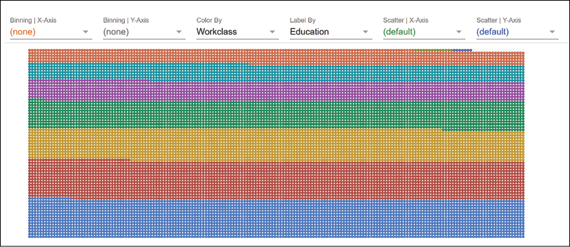
Figure 5.4: The interface of Facets

We are now ready to analyze the data.

Analyzing the training data with Facets

We will limit our analysis to trying to find critical features that determine the income level of a person. We will strive to avoid features that could offend the people using the AI application.

If we exclude homeless people and billionaires, we will find that for the population of people working around the world, two significant features in this dataset (age and years in education) produce interesting results.

To visualize these two features, we will display the first feature: age. Choose the Age option under Binning | X-Axis and Over-50K in the Color By field, as shown in Figure 5.5:

Figure 5.5: The Dive visualization tool of Facets

You will see age groups in the x axis and two-color bars for each group. The lower portion of the bars is blue (see the following color plot), representing lower income values. The higher part of the bars is red, representing the higher income values. Look carefully at the following visualization:

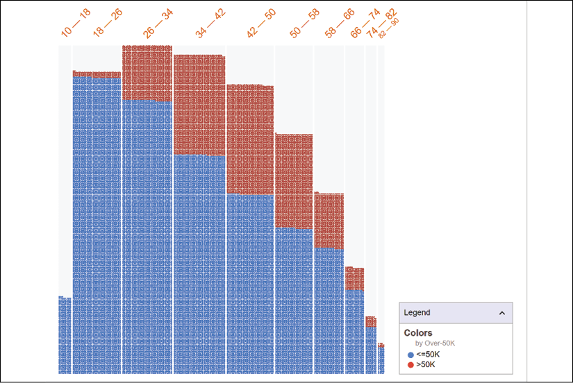
Figure 5.6: Chart showing that as age increases, so does income

The following universal principals clearly appear:

• A ten-year-old person earns less than a person who is 30 years old
• A person who is over 70 years old is more likely than not to be retired and have lower income than a person who is 40 years old
• The income curve increases from childhood to adulthood, reaches a peak, and then goes slowly down with age

This natural physical reality provides reliable inferences.

Now, let's add the number of years of education (Education-Num) to Binning | Y-Axis:

Figure 5.7: Defining the y axis of Dive

The visualization changes and provides bins per years of education. The x axis represents the age of the population analyzed in years binned.

The y axis bins represent the number of years of education of the person in question. For example, 12 means 12 years of education. 15-16 means 15 to 16 years of education (such as a Ph.D., for example).

The bottom section (colored blue in the color image) of each bar represents an income of <50K. The top section (colored red in the color image) represents an income of >50K:

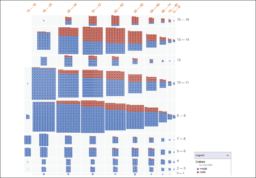
Figure 5.8: Higher education (on the y axis) leads to higher income (on the x axis)

Several additional universal principals appear, as follows:

• The longer a person studies, the more that person will earn. For example, in the bin of 15-16 years of education, you can see that there are practically only individuals with an income of >50K.
• Learning can be acquired through experience. For example, in the range of 8-9 years of education, you can see that income increases slightly with years of experience. In the range of 13-14 years of education, the progression is faster due to better job opportunities.
• After a few years of experience, a person with higher education will make more income. This is linked to learning acquired through experience.
• The age factor is intensified by education and experience, which explains why the higher-income portion of the bars increase in a significant way for those having between 13 and 17 years of education starting at age 30, for example.

Can an ML algorithm verify this hypothesis? Are there limits? Let's check the anticipated outputs with a k-means clustering program.

Verifying the anticipated outputs

In the last section, we found two key features that determine the income of a given person: age and number of years of education. These two features do not include the controversial features we seek to avoid.

We will extract the age and education-num columns from the adult.data file containing the U.S. census data. Then we create a file with those two columns named data_age_education.csv. The header includes the two features and the corresponding data from the original data file:

age,numed
39,13
50,13
38,9
53,7
28,13
37,14
...

The file is ready, and we can train it with an ML algorithm.

Using KMC to verify the anticipated results

We will build a separate Python program with a k-means clustering (KMC) algorithm before continuing with the WIT_Model_Comparison_Ethical.ipynb notebook. The goal is to divide the data into two categories: income above 50K, and equal to and below 50K. Once the data is classified, we will label it.

Open /KMC/k-means_clustering.py.

We will first import the modules we need:

from sklearn.cluster import KMeans # for the KMC
import pandas as pd # to load the data into DataFrames
import pickle # to save the trained KMC model and
              # load it to generate the outputs
import numpy as np # to manage arrays

Now, we read the data file containing the two key features we will classify and label:

# I. Training the dataset
dataset = pd.read_csv('data_age_education.csv')
print(dataset.head())
print(dataset)

The first lines of the output show that the DataFrame contains the data we will use:

   age  numed
0   39     13
1   50     13
2   38      9
3   53      7
4   28     13
...

We will now insert the KMC:

# creating the classifier
k = 2
kmeans = KMeans(n_clusters=k)

k = 2 defines the number of clusters we want to calculate. One cluster will be the records labeled >50K. The other cluster will contain the records labeled <=50K.

Each cluster is built around a geometric center, a centroid. The centroid is the center of the mean of the sum of distances of x data points of each cluster.

The variables used by the k-means estimator are as follows:

• k is the number of clusters
• u is the centroid of each cluster
• x represents each of the data points from 1 to n

The Euclidean distance, in one dimension, is the distance between two points x and y, expressed as follows:

The closer the points are to each other and to the centroid of a cluster, the higher the accuracy of the KMC is for that cluster. We can now plug the variables in the following equation:

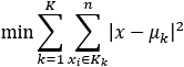
Lloyd's algorithm will use this type of equation to optimize the clusters.

The program will now run to fit the dataset and optimize the clusters:

# k-means clustering algorithm
kmeans = kmeans.fit(dataset)        # Computing k-means clustering
gcenters = kmeans.cluster_centers_  # The geometric centers or
                                    # centroids

The centroids are displayed by the program once the training is over:

print("The geometric centers or centroids:")
print(gcenters)

The output is as follows:

The geometric centers or centroids:
[[52.02343227 10.17473778]
 [29.12992991 10.01454127]]

Note that the value of the centroids can vary from calculation to calculation.

The program now saves the model:

# save model
filename = "kmc_model.sav"
pickle.dump(kmeans, open(filename, 'wb'))
print("model saved")

The program can now load the trained model:

# II. Testing the dataset
# dataset = pd.read_csv('data.csv')
kmeans = pickle.load(open('kmc_model.sav', 'rb'))

We create an array to store our predictions and activate the prediction variable:

# making and saving the predictions
kmcpred = np.zeros((32563, 3))
predict = 1

The program now makes predictions on the dataset, labels the records, and saves the results in a .csv file:

if predict == 1:
    for i in range(0, 32560):
        xf1 = dataset.at[i, 'age']; xf2 = dataset.at[i, 'numed'];
        X_DL = [[xf1, xf2]]
        prediction = kmeans.predict(X_DL)
        # print(i+1, "The prediction for", X_DL, " is:",
        #       str(prediction).strip('[]'))
        # print(i+1, "The prediction for", str(X_DL).strip('[]'),
        #       " is:", str(prediction).strip('[]'))
        p = str(prediction).strip('[]')
        p = int(p)
        kmcpred[i][0] = int(xf1)
        kmcpred[i][1] = int(xf2)
        kmcpred[i][2] = p
np.savetxt('ckmc.csv', kmcpred, delimiter=',', fmt='%d')
print("predictions saved")

The file contains the two key features and the labels, respectively, age, education-num, and the binary class (0 or 1):

39,13,1
50,13,0
38,9,1
53,7,0
28,13,1

Note that the label values can change from one to another for a given class.

We will now upload the ckmc.csv file to a spreadsheet that already contains the adult.data file, a sample of the U.S. census data with ML labels.

Analyzing the output of the KMC algorithm

In the last section, we produced the ckmc.csv file. We can now compare the results obtained by the KMC and the results produced by the ML algorithms used to create adult.data, the original trained U.S. census data file used in this chapter.

We will first load the adult.data file, as displayed in the following three screenshots. The adult data tab of the spreadsheet of data_analysis.xlsx is available in the directory of this chapter. The following table contains the first columns:

This table contains the following columns:

The last columns of the adult.data file contain the controversial data for which we need to make a decision regarding its usage:

Now, we insert the label of the initial dataset, Over-50K, and the three columns of ckmc.csv, the output of the KMC verification program:

We will analyze two samples to explain the results, starting with sample 1.

Sample 1 – Filtering by age 30 to 39 and 14 years of education

We will filter the data using the spreadsheet's filters to focus on the people who are between 30 and 39 years old. We also select 14 years of education in the Education-Num field. 14 years is about what it takes to obtain a bachelor's or a master's degree.

When we look at the first 4 records, we see that our KMC predicts 1, >50K for all 4 records:

However, you will notice the algorithms used to predict that the income of the people are not stable with these features.

The adult.names file contains a description of the ML algorithms used and the error rate. For example, the following excerpt of adult.names provides a description of the work accomplished:

|    Algorithm               Error
| -- ----------------        -----
| 1  C4.5                    15.54
| 2  C4.5-auto               14.46
| 3  C4.5 rules              14.94
| 4  Voted ID3 (0.6)         15.64
| 5  Voted ID3 (0.8)         16.47
| 6  T2                      16.84
| 7  1R                      19.54
| 8  NBTree                  14.10
| 9  CN2                     16.00
| 10 HOODG                   14.82
| 11 FSS Naive Bayes         14.05
| 12 IDTM (Decision table)   14.46
| 13 Naive-Bayes             16.12
| 14 Nearest-neighbor (1)    21.42
| 15 Nearest-neighbor (3)    20.35
More...

We will name these algorithms the USC algorithms (U.S. census algorithms) in this section.

For each result, we will state that the >50K column prediction is positive when income is >50K and negative if the income is <=50K.

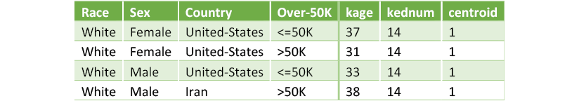
The Over-50K column resulting from the original data leads to several questions:

• Line 1 shows a positive result for the KMC but not for the USC.
• Could race be a discriminating feature? Not in this case, since all four lines contain White as the feature for race.
• Could work class be a discriminating feature? Not in this case, since the first two lines are private and USC does not produce the same label.
• Could the sex of the person make a difference? Not in this case, since the first two lines are Female, and the two other lines are Male.
• Could the country of origin make a difference? Not in this case, because the fourth person in this sample comes from Iran and shows a positive result for USC.
• The relationship or marital status makes no sense, so it is ignored for this case.

Clearly, the KMC shows a logical result in this age group for people who have a master's degree or above. However, USC cannot explain why the results are not stable.

In this case, our implementation of XAI has led to several interesting questions on how to predict the income of the people based on the information provided.

Let's add a controversial feature, such as race.

Sample 2 – Filtering by age 30 to 39, 14 years of education, and "race"="black" or "race"="white"

On lines 13,372 and 13,378, we have two interesting observations:

Race (Black or White) makes no sense here. Black is positive for USC and negative for White. Opposite cases can be found for USC. The KMC algorithm provides positive values that seem logical.

We could examine hundreds of samples and still not reach conclusive proof that features other than age and the level of education provide highly accurate results.

Let's conclude this analysis.

Conclusion of the analysis

We have explored the original adult.data file and have reached the following conclusions:

• The U.S. census data represents best what it was designed for: a census of the population of the United States
• The adult.data U.S. census sample contains labeled data showing how to use ML algorithms for various tasks
• The adult.data file provides a unique dataset for XAI

The team that used the U.S. census data to test ML programs did an excellent job of showing how AI can be applied to datasets.

XAI shows that the data contained in the adult.data file is insufficient to predict the income of a person.

Using a customized what-if approach with Facets Dive and a KMC, we explored two key features of the adult.data file: age and the number of years of education. The results were logical and showed no bias. However, better results could be obtained with more information on a person.

It appears that in real-life projects, two more key features are required to produce better income predictions:

• The level of consistency between the education of a person and their work experience. If a person has a master's degree in mathematics, for example, but works as a librarian for some reason or another, there will be a significant income variance.
• The number of successful years of experience in a given field is a crucial factor when recruiting a person.

We know that age, level of education, years of successful experience, and the level of consistency between our education and our job constitute the pillars of our market value.

We now know that key information is missing in the adult.data dataset and the controversial fields do not really explain the differences between the labels.

We will thus transform the controversial columns into cultural columns that provide interesting information on a person, if the person consents to offering this private data.

Transforming the input data

We will now suppress the controversial data, keeping the same number of fields but replacing the field names with other cultural information before using Google's WIT tool. The motivation isn't to obtain better numerical results. These fields provide a better, more human background to a person that can help predict if that person's income is high or low. The present practice of the market is to ignore discriminatory information on a person and focus on the real qualities required to get a job done.

The original data contained the following columns:

csv_columns = ["Age", "Workclass", "fnlwgt", "Education",
               "Education-Num", "Marital-Status", "Occupation",
               "Relationship", "Race", "Sex", "Capital-Gain",
               "Capital-Loss", "Hours-per-week", "Country",
               "Over-50K"]

The transformed data contains the following columns:

csv_columns = ["Age", "Purchasing", "fnlwgt", "Education",
               "Education-Num", "media", "Occupation", "transport",
               "reading", "traveling", "Capital-Gain",
               "Capital-Loss", "Hours-per-week", "Country",
               "Over-50K"]

The following descriptions of the transformed features are merely speculative at this point. We would have to obtain real data from a random sample of a cultural survey. Then we would have to implement ML algorithms to see which features have an impact on income predictions. We would also have to add more features if the results weren't accurate.

We consider the following new fields as an excellent way to approach XAI for educational purposes without having to use controversial information:

• Workclass becomes purchasing: Purchasing contains information on purchasing habits. The behavior of a person who mostly goes to markets and not supermarkets can be an income indicator, for example. We define our new Purchasing field as:

  Purchase = {shops, markets, malls, supermarkets}

• Marital-Status becomes media: Media describes the way a person accesses music and movies. We define our new media field as:

  Media = {DVD, live, social_networks, television, theaters, websites}

  A person who mostly goes to a theater to see a movie spends more money than a person who mostly watches movies on television.

• Relationship becomes transport: Transport shows how a person goes from one location to another. A person who drives an expensive car and never takes a bus spends more money than a person who either walks or takes a bus. We define our new transport field as:

  Transport = {walking, running, cycling, bus, car}

• Race becomes reading: A person who reads books and magazines versus a person who only reads websites could be more educated. We define our new reading field as:

  Reading = {books, magazines, television, websites}

• Sex becomes traveling preferences, in terms of physical activities: One person might mostly prefer action, such as surfing, running, swimming, and other structured physical activities. Another person might mostly prefer to discover new horizons, such as treks in distant mountains or jungles. Swimming at a local pool costs less than treks in distant countries, for example. We define our new traveling field as:

  Traveling = {action, adventures}

Note that some of the features of the original content are still present in some of these fields, creating some useful noise in the dataset.

Our customized what-if method leads to the suppression of controversial fields in the adult.data dataset and we replaced them with cultural features that will not offend anybody. On top of that, our cultural features make more sense when analyzing a person's level of income.

We will now explore WIT applied to an entertaining ethical dataset.

WIT applied to a transformed dataset

We carried out a full what-if XAI investigation from scratch. We then transformed the data of the U.S. census sample. Now, let's explore the transformed data using Google's WIT tool.

The first step is to load our transformed dataset from GitHub, or you can choose to use Google Drive by setting repository to "google":

# @title Importing data <br>
# Set repository to "github"(default) to read the data
# from GitHub <br>
# Set repository to "google" to read the data
# from Google {display-mode: "form"}
import os
from google.colab import drive
# Set repository to "github" to read the data from GitHub
# Set repository to "google" to read the data from Google
repository = "github"
if repository == "github":
  !curl -L https://raw.githubusercontent.com/PacktPublishing/Hands-On-Explainable-AI-XAI-with-Python/master/Chapter05/adult_train.csv --output "adult_train.csv"
  dtrain = "/content/adult_train.csv"
  print(dtrain)
if repository == "google":
  # Mounting the drive. If it is not mounted, a prompt
  # will provide instructions.
  drive.mount('/content/drive')
  # Setting the path for each file
  dtrain = '/content/drive/My Drive/XAI/Chapter05/adult_train.csv'
  print(dtrain)

We comment out the former CSV column definitions and define our feature names:

# @title Read training dataset from CSV {display-mode: "form"}
import pandas as pd
# Set the path to the CSV containing the dataset to train on.
csv_path = dtrain
# Set the column names for the columns in the CSV.
# If the CSV's first line is a header line containing
# the column names, then set this to None.
csv_columns = ["Age", "Purchasing", "fnlwgt", "Education",
               "Education-Num", "media", "Occupation", "transport",
               "reading", "traveling", "Capital-Gain",
               "Capital-Loss", "Hours-per-week", "Country",
               "Over-50K"]
'''
csv_columns = ["Age", "Workclass", "fnlwgt", "Education",
               "Education-Num", "Marital-Status", "Occupation",
               "Relationship", "Race", "Sex", "Capital-Gain",
               "Capital-Loss", "Hours-per-week", "Country",
               "Over-50K"]
'''

We now display the transformed data:

# Read the dataset from the provided CSV and print out
# information about it.
df = pd.read_csv(csv_path, names=csv_columns, skipinitialspace=True)
df

The following output shows our transformed data:

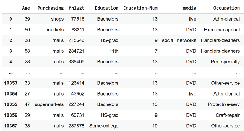
Figure 5.9: Transformed data

The program now specifies the label column, which has not been transformed. We respect the original labeling of the dataset and the comments from the Google team:

# @title Specify input columns and column to predict
# {display-mode: "form"}
import numpy as np
# Set the column in the dataset you wish for the model to predict
label_column = 'Over-50K'
# Make the label column numeric (0 and 1), for use in our model.
# In this case, examples with a target value of '>50K' are
# considered to be in the '1' (positive) class and all other
# examples are considered to be in the '0' (negative) class.
make_label_column_numeric(df, label_column, lambda val: val == '>50')

Now, we insert our cultural features in place of the original data:

# Set list of all columns from the dataset we will use for
# model input.
input_features = ['Age', 'Purchasing', 'Education', 'media',
                  'Occupation', 'transport', 'reading', 'traveling',
                  'Capital-Gain', 'Capital-Loss', 'Hours-per-week',
                  'Country']

Our customized XAI investigation showed that we need additional data to make accurate income predictions. We thus applied an ethical approach—the controversial fields have been removed. The cultural data is random because we have seen that they are not significant when compared to the level of education. We know that a person with a master's degree or a Ph.D. has a higher probability of earning more than a person with a tenth-grade education. This feature will weigh heavily on the income level.

We now have an ethical dataset to explore Google's innovative WIT with.

The program now creates a list with all of the input features:

features_and_labels = input_features + [label_column]

The data has to be converted into datasets that are compatible with TensorFlow estimators:

# @title Convert dataset to tf.Example protos
# {display-mode: "form"}
examples = df_to_examples(df)

We now run the linear classifier as implemented by Google's team:

# @title Create and train the linear classifier
# {display-mode: "form"}
num_steps = 2000 # @param {type: "number"}
# Create a feature spec for the classifier
feature_spec = create_feature_spec(df, features_and_labels)
# Define and train the classifier
train_inpf = functools.partial(tfexamples_input_fn, examples,
                               feature_spec, label_column)
classifier = tf.estimator.LinearClassifier(
    feature_columns=create_feature_columns(input_features,
        feature_spec))
classifier.train(train_inpf, steps=num_steps)

We then run the deep neural network (DNN) as implemented by Google's team:

# @title Create and train the DNN classifier {display-mode: "form"}
num_steps_2 = 2000 # @param {type: "number"}
classifier2 = tf.estimator.DNNClassifier(
    feature_columns=create_feature_columns(input_features,
        feature_spec), hidden_units=[128, 64, 32])
classifier2.train(train_inpf, steps=num_steps_2)

We will explore TensorFlow's DNN and others in more detail in Chapter 6, AI Fairness with Google's What-If Tool (WIT).

For now, move on and display the trained dataset in Google's implementation of Facets Dive.

We choose the number of data points we wish to explore and the height of the tool:

num_datapoints = 2000    # @param {type: "number"}
tool_height_in_px = 1000 # @param {type: "number"}

We import the visualization witwidget modules:

from witwidget.notebook.visualization import WitConfigBuilder
from witwidget.notebook.visualization import WitWidget

For our example, we'll use our transformed dataset to test the model:

dtest = dtrain
# Load up the test dataset
test_csv_path = dtest
test_df = pd.read_csv(test_csv_path, names=csv_columns,
                      skipinitialspace=True, skiprows=1)
make_label_column_numeric(test_df, label_column,
                          lambda val: val == '>50K.')
test_examples = df_to_examples(test_df[0:num_datapoints])

We finally set up the tool and display the WIT visualization interface:

config_builder = WitConfigBuilder(
    test_examples[0:num_datapoints]).set_estimator_and_feature_spec(
    classifier, feature_spec).set_compare_estimator_and_feature_spec(
    classifier2, feature_spec).set_label_vocab(
    ['Under 50K', 'Over 50K'])
a = WitWidget(config_builder, height=tool_height_in_px)

You are ready to explore the results with Google's implementation of Facets in WIT from a user's perspective:

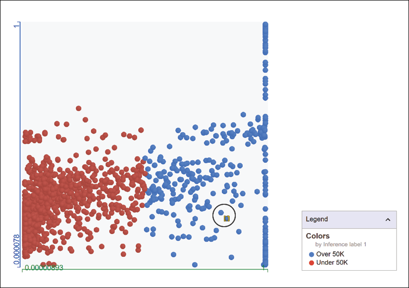
Figure 5.10: Exploring results with WIT using Facets

The data point chosen is a >50K point in the blue (see color image) area. We will now look at the features of this person:

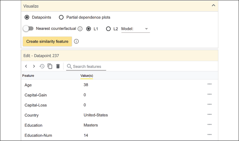
Figure 5.11: The feature interface of WIT

The information provides an interesting perspective. Although we replaced several fields of the original data with cultural fields, higher education for a person between 30 and 39 leads to higher income in this case. Our cultural features did not alter the predicted income level of this person:

Figure 5.12: Cultural features in WIT that did not modify the predictions

We know that we cannot expect sufficiently accurate results until we add other fields such as the number of years of job experience in the area, or the presence of a college degree.

We can use WIT to prove this by activating the nearest counterfactual data point:

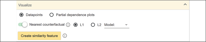
Figure 5.13: Activating the nearest counterfactual option

A new point appears in the <=50K area of the visualization module:

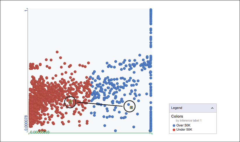
Figure 5.14: Visualizing the nearest counterfactual data point

This excellent tool has displayed a data point that should have been >50 but isn't. You can investigate hundreds of data points and find out which features count the most for a given model.

The information of the first data point we chose automatically displays the counterfactual data point so that we can compare the features:

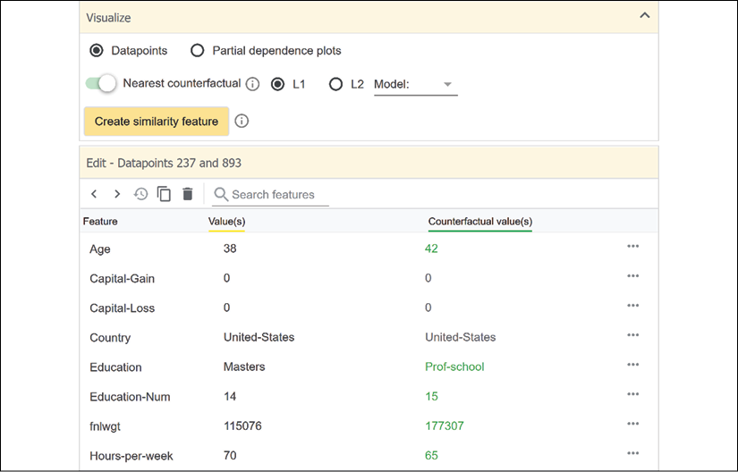
Figure 5.15: Comparing the features of a data point with a counterfactual data point

We can make some observations without drawing any conclusions until we have more information on the careers of these two people:

• The counterfactual age value is not in the 30-39 age group we targeted. However, this is not a valid explanation since the graph in the Analyzing the training data with Facets section of this chapter showed that the 42-50 age group with 14+ years of education constitutes a higher proportion of >50K earners than the 34-42 age group with 14+ years of education.
• They both have studied for 14+ years.
• One person works 70 hours and the other 65 hours. That does not mean much, with just a 5-hour difference. We have no information to confirm that those 5 hours are paid as overtime work. We would need to have this information to be able to make such a conclusion.
• We don't know how much they both actually earn. Maybe the counterfactual data point represents a person who makes 50K, which puts the value in the <=50K class. Perhaps the person who makes >50K only earns 50.5K. The border between the two classes is very precise, although the data isn't.

We recommend that you spend as much time as necessary drawing exciting what-if conclusions that will boost your XAI expertise.

In this section, we loaded the dataset and transformed and defined the new features. We then ran a linear estimator and a DNN. We displayed the data points in WIT's visualization module to investigate factual and counterfactual data points.

Summary

In this chapter, we first explored the moral and ethical issues involved in an AI project. We asked ourselves whether using certain features could offend the future users of our program.

We examined the legal issues of some of the information in a dataset from a legal perspective. We discovered that the legal use of information depends on who processes it and how it is collected. The United States government, for example, is entitled to use data on certain features of a person for a U.S. census survey.

We found that even if a government can use specific information, this doesn't mean that a private corporation can use it. This is illegal for many other applications. Both U.S. and European legislators have enacted strict privacy laws and make sure to apply them.

The ML perspective showed that the key features, such as age and the level of education, provide interesting results using a KMC algorithm. We built a KMC algorithm and trained on age and level of education. We saved the model and ran it to produce our labels. These labels provided a logical explanation. If you have a high level of education, such as 14+ years of overall education, for example, you are more likely to have a higher income than somebody with less education.

The KMC algorithm detected that higher education in age groups with some years of experience provides a higher income. However, the same customized XAI approach showed that additional features were required to predict the income level of a given person.

We suppressed the controversial features of the original dataset and inserted random cultural features.

We trained the transformed data with a linear classifier and a DNN, leaving the initial labels as they were.

Finally, we used WIT's visualization modules to display the data. We saw how to use WIT to find explanations for factual and counterfactual data points.

In the next chapter, AI Fairness with Google's What-If Tool (WIT), we will build an ethical XAI investigation program.

Questions

1. Moral considerations mean nothing in AI as long as it's legal. (True|False)
2. Explaining AI with an ethical approach will help users trust AI. (True|False)
3. There is no need to check whether a dataset contains legal data. (True|False)
4. Using machine learning algorithms to verify datasets is productive. (True|False)
5. Facets Dive requires an ML algorithm. (True|False)
6. You can anticipate ML outputs with Facets Dive. (True|False)
7. You can use ML to verify your intuitive predictions. (True|False)
8. Some features in an ML model can be suppressed without changing the results. (True|False)
9. Some datasets provide accurate ML labels but inaccurate real-life results. (True|False)
10. You can visualize counterfactual datapoints with WIT. (True|False)

References

Google's WIT income classification example can be found at https://pair-code.github.io/what-if-tool/index.html#demos

Further reading

For more on k-means clustering, see the following link:

https://scikit-learn.org/stable/modules/generated/sklearn.cluster.KMeans.html