2

White Box XAI for AI Bias and Ethics

AI provides complex algorithms that can replace or emulate human intelligence. We tend to think that AI will spread unchecked by regulations. Without AI, corporate giants cannot process the huge amounts of data they face. In turn, ML algorithms require massive amounts of public and private data for training purposes to guarantee reliable results.

However, from a legal standpoint, AI remains a form of automatic processing of data. As such, just like any other method that processes data automatically, AI must follow the rules established by the international community, which compel AI designers to explain how decisions are reached. Explainable AI (XAI) has become a legal obligation.

The legal problem of AI worsens once we realize that for an algorithm to work, it requires data, that is, huge volumes of data. Collecting data requires access to networks, emails, text messages, social networks, hard disks, and more. By its very nature, processing data automatically requires access to that same data. On top of that, users want quick access to web sites that are increasingly driven by AI.

We need to add ethical rules to our AI algorithms to avoid being slowed down by regulations and fines. We must be ready to explain the alleged bias in our ML algorithms. Any company, whether huge or tiny, can be sued and fined.

This puts huge pressure on online sites to respect ethical regulations and avoid bias. In 2019, the U.S. Federal Trade Commission (FTC) and Google settled for USD 170,000,000 for YouTube's alleged violations of children's privacy laws. In the same year, Facebook was fined USD 5,000,000,000 by FTC for violating privacy laws. On January 21, 2019, a French court applied the European General Data Protection Regulation (GDPR) and sentenced Google to pay a €50,000,000 fine for a lack of transparency in their advertising process. Google and Facebook stand out because they are well known. However, every company faces these issues.

The roadmap of this chapter becomes clear. We will determine how to approach AI ethically. We will explain the risk of bias in our algorithms when an issue comes up. We will apply explainable AI as much as possible, and as best as we possibly can.

We will start by judging an autopilot in a self-driving car (SDC) in life-and-death situations. We will try to find how an SDC driven by an autopilot can avoid killing people in critical traffic cases.

With these life-and-death situations in mind, we will build a decision tree in an SDC's autopilot. Then, we will apply an explainable AI approach to decision trees.

Finally, we will learn how to control bias and insert ethical rules in real time in the SDC's autopilot.

This chapter covers the following topics:

• The Moral Machine, Massachusetts Institute of Technology (MIT)
• Life and death autopilot decision making
• The ethics of explaining the moral limits of AI
• An explanation of autopilot decision trees
• A theoretical description of decision tree classifiers
• XAI applied to an autopilot decision tree
• The structure of a decision tree
• Using XAI and ethics to control a decision tree
• Real-time autopilot situations

Our first step will be to explore the challenges an autopilot in an SDC faces in life and death situations.

Moral AI bias in self-driving cars

In this section, we will explain AI bias, morals, and ethics. Explaining AI goes well beyond understanding how an AI algorithm works from a mathematical point of view to reach a given decision. Explaining AI includes defining the limits of AI algorithms in terms of bias, moral, and ethical parameters. We will use AI in SDCs to illustrate these terms and the concepts they convey.

The goal of this section is to explain AI, not to advocate the use of SDCs, which remains a personal choice, or to judge a human driver's decisions made in life and death situations.

Explaining does not mean judging. XAI provides us with the information we need to make our decisions and form our own opinions.

This section will not provide moral guidelines. Moral guidelines depend on cultures and individuals. However, we will explore situations that require moral judgments and decisions, which will take us to the very limits of AI and XAI.

We will provide information for each person so that we can understand the complexity of the decisions autopilots face in critical situations.

We will start by diving directly into a complex situation for a vehicle on autopilot.

Life and death autopilot decision making

In this section, we will set the grounds for the explainable decision tree that we will implement in the subsequent sections. We will be facing life and death situations. We will have to analyze who might die in an accident that cannot be avoided.

This section uses MIT's Moral Machine experiment, which addresses the issue of how an AI machine will make moral decisions in life and death situations.

To understand the challenge facing AI, let's first go back to the trolley problem.

The trolley problem

The trolley problem takes us to the core of human decisions. Should we decide on a purely utilitarian basis, maximizing utility above anything else? Should we take deontological ethics—that is, actions based on moral rules—into account? The trolley problem, which was first expressed more than 100 years ago, creates a dilemma that remains difficult to solve since it leads to subjective cultural and personal considerations.

The trolley problem involves four protagonists:

• A runaway trolley going down a track: Its brakes have failed, and it is out of control.
• A group of five people at a short distance in front of the trolley: They will be killed if the trolley continues on its track.
• One person on a sidetrack.
• You, standing next to a lever: If you don't pull the lever, five people will die. If you pull the lever, one person will die. You only have a few seconds to make your decision.

In the following diagram, you can see the trolley on the left; you in the middle, next to the lever; the five people that will be killed if the trolley stays on the track; and the person on the sidetrack:

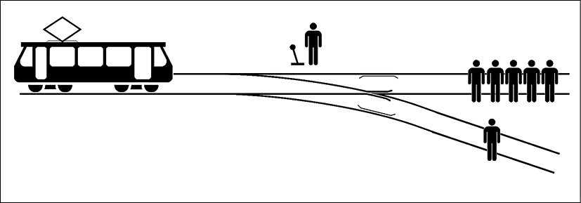
Figure 2.1: The trolley problem
!Original: McGeddonVector: Zapyon / CC BY-SA (https://creativecommons.org/licenses/by-sa/4.0)

This mind experiment consists of imagining numerous situations such as:

• Five older people on the track and one child on the sidetrack
• Five women on the track and one man on the sidetrack
• A young family on the track and an elderly person on the sidetrack
• Many more combinations

You must decide whether to pull the lever or not. You must determine who will die. Worse, you must decide how your ML autopilot algorithm will make decisions in an SDC when facing life and death situations.

Let's explore the basis of moral-based decision making in SDCs.

The MIT Moral Machine experiment

The MIT Moral Machine experiment addresses the trolley problem transposed into our modern world of self-driving autopilot algorithms. The Moral Machine experiment explored millions of answers online in many cultures. It presents situations you must judge. You can test this on the Moral Machine experiment site at http://moralmachine.mit.edu/.

The Moral Machine experiment confronts us with machine-made moral decisions. An autopilot running calculations does not think like a human in the trolley problem. An ML algorithm thinks in terms of the rules we set. But how can we set them if we do not know the answers ourselves? We must answer this question before putting our autopilot algorithms on the market. Hopefully, by the end of this chapter, you will have some ideas on how to limit such situations.

The Moral Machine experiment extends the trolley problem further. Should we pull the lever and stop implementing AI autopilot algorithms in cars until they are ready in a few decades?

If so, many people will die because a well-designed autopilot saves some lives but not others. An autopilot is never tired. It is alert and respects traffic regulations. However, autopilots will face the trolley problem and calculation inaccuracies.

If we do not pull the lever and let autopilots run artificial intelligence programs, autopilots will start making life and death decisions and will kill people along the way.

The goal of this section and chapter is not to explore every situation and suggest rules. Our primary goal is limited to explaining the issues and possibilities so that you can judge what is best for your algorithms. We will, therefore, be prepared to build a decision tree for the autopilot in the next section.

Let's now explore a life and death situation to prepare ourselves with the task of building a decision tree.

Real life and death situations

The situation described in this section will prepare us to design tradeoffs in moral decision making in autopilots. I used the MIT Moral Machine to create the two options an AI autopilot can take when faced with the situation shown in the following diagram:

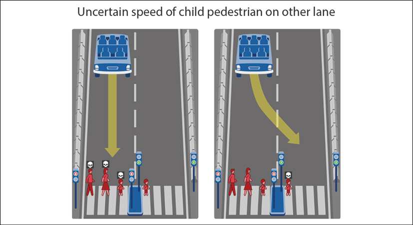
Figure 2.2: A situation created using the MIT Moral Machine

For several possible reasons, the car shown in the preceding diagram cannot avoid either going straight ahead or changing lanes:

• Brake failure.
• The SDC's autopilot did not identify the pedestrians well or fast enough.
• The AI autopilot is confused.
• The pedestrians on the left side of the diagram suddenly crossed the road when the traffic light was red for pedestrians.
• It suddenly began to rain, and the autopilot failed to give the human driver enough time to react. Rain obstructs an SDC's sensors. The cameras and radars can malfunction in this case.
• Another reason.

Many factors can lead to this situation. We will, therefore, refer to this situation by stating that whatever the reason, the car does not have enough time to stop before reaching the traffic light.

We will try to provide the best answer to the situation described in the preceding diagram. We will now approach this from an ethical standpoint.

Explaining the moral limits of ethical AI

We now know that a life and death situation that involves deaths, no matter what decision is made, will be subjective in any case. It will depend more on cultural and human values than on pure ML calculations.

Ethically explaining AI involves honesty and transparency. By doing so, we are honest and transparent. We explain why we, as humans, struggle with this type of situation, and ML autopilots cannot do better.

To illustrate this, let's analyze a potential real-life situation.

On the left side of Figure 2.3, we see a car on autopilot using AI that is too close to a pedestrian walk to stop. We notice that the traffic light is green for the car and red for pedestrians. A death symbol is on the man, the woman, and the child because they will be seriously injured if the car hits them:

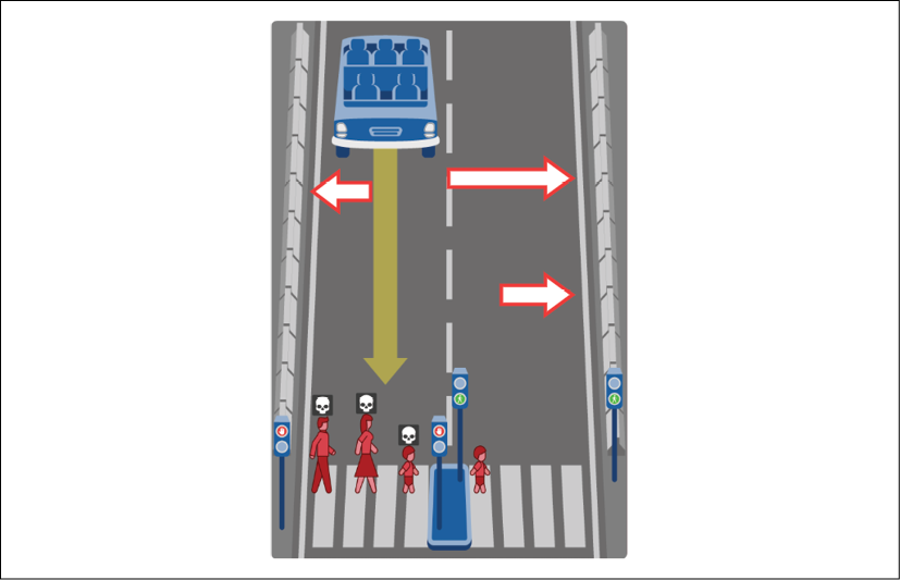
Figure 2.3: A life and death situation

A human driver could try to:

• Immediately turn the steering wheel to the left to hit the wall with the brakes on and stop the car. This manual maneuver automatically turns the autopilot off. Of course, the autopilot could be dysfunctional and not stop. Or, the car would continue anyway and hit the pedestrians.
• Immediately do the same maneuver but instead cross lanes to the other side. Of course, a fast incoming car could be coming in the opposite direction. The car could slide, miss the wall, and hit the child anyway on the other lane.

A human driver could try to change lanes to avoid the three pedestrians and only risk injuring or killing one on the other lane:

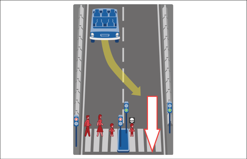
Figure 2.4: Swerving to another lane

The driver might be able to avoid the pedestrian on the other lane. In that case, it would be risking one life instead of three.

What would you do?

I do not think we can ask an AI program to make that choice. We need to explain why and find a way to offer a solution to this problem before letting driverless SDCs roam freely around a city!

Let's view this modern-day trolley problem dilemma from an ML perspective.

Standard explanation of autopilot decision trees

An SDC contains an autopilot that was designed with several artificial intelligence algorithms. Almost all AI algorithms can apply to an autopilot's need, such as clustering algorithms, regression, and classification. Reinforcement learning and deep learning provide many powerful calculations.

We will first build an autopilot decision tree for our SDC. The decision tree will be applied to a life and death decision-making process.

Let's start by first describing the dilemma from a machine learning algorithm's perspective.

The SDC autopilot dilemma

The decision tree we are going to create will be able to reproduce an SDC's autopilot trolley problem dilemma. We will adapt to the life and death dilemma in the Moral AI bias in self-driving cars section of this chapter.

The decision tree will have to decide if it stays in the right lane or swerves over to the left lane. We will restrict our experiment to four features:

• f1: The security level on the right lane. If the value is high, it means that the light is green for the SDC and no unknown objects are on the road.
• f2: Limited security on the right lane. If the value is high, it means that no pedestrians might be trying to cross the street. If the value is low, pedestrians are on the street, or there is a risk they might try to cross.
• f3: Security on the left lane. If the value is high, it would be possible to change lanes by swerving over to the other side of the road and that no objects were detected on that lane.
• f4: Limited security on the left lane. If the value is low, it means that pedestrians might be trying to cross the street. If the value is high, pedestrians are not detected at that point.

Each feature has a probable value between 0 and 1. If the value is close to 1, the feature has a high probability of being true. For example, if f1 = 0.9, this means that the security of the right lane is high. If f1 = 0.1, this means that the security of the right lane is most probably low.

We will import 4,000 cases involving all four features and their 2 possible labeled outcomes:

• If label = 0, the best option is to stay in the right lane
• If label = 1, the best option is to swerve to the left lane

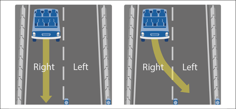
Figure 2.5: Autopilot lane changing situation

We will start by importing the modules required to run our decision tree and XAI.

Importing the modules

In this section, we will build a decision tree with the Google Colaboratory notebook. Go to Google Colaboratory, as explained in Chapter 1, Explaining Artificial Intelligence with Python. Open Explainable_AI_Decision_Trees.ipynb.

We will be using the following modules in Explainable_AI_Decision_Trees.ipynb:

• numpy to analyze the structure of the decision tree
• pandas for data manipulation
• matplotlib.pyplot to plot the decision tree and create an image
• pickle to save and load the decision tree estimator
• sklearn.tree to create the decision tree classifier and explore its structure
• sklearn.model_selection to manage the training and testing data
• metrics is scikit-learn's metrics module and is used to measure the accuracy of the training process
• os for the file path management of the dataset

Explainable_AI_Decision_Trees.ipynb starts by importing the modules mentioned earlier:

import numpy as np
import pandas as pd
import matplotlib.pyplot as plt
import pickle
from sklearn.tree import DecisionTreeClassifier, plot_tree
from sklearn.model_selection import train_test_split
from sklearn import metrics
import os

Now that the modules are imported, we can retrieve the dataset.

Retrieving the dataset

There are several ways to retrieve the dataset file, named autopilot_data.csv, which can be downloaded along with the code files of this chapter.

We will use the GitHub repository:

# @title Importing data <br>
# Set repository to "github"(default) to read the data
# from GitHub <br>
# Set repository to "google" to read the data
# from Google {display-mode: "form"}
import os
from google.colab import drive
# Set repository to "github" to read the data from GitHub
# Set repository to "google" to read the data from Google
repository = "github"
if repository == "github":
  !curl -L https://raw.githubusercontent.com/PacktPublishing/Hands-On-Explainable-AI-XAI-with-Python/master/Chapter02/autopilot_data.csv --output "autopilot_data.csv"
  # Setting the path for each file
  ip = "/content/autopilot_data.csv"
  print(ip)

The path of the dataset file will be displayed:

/content/autopilot_data.csv

Google Drive can also be activated to retrieve the data. The dataset file is now imported. We will now process it.

Reading and splitting the data

We defined the features in the introduction of this section. f1 and f2 are the probable values of the security on the right lane. f3 and f4 are the probable values of the security on the left lane. If the label is 0, then the recommendation is to stay in the right lane. If the label is 1, then the recommendation is to swerve over to the left lane.

The file does not contain headers. We first define the names of the columns:

col_names = ['f1', 'f2', 'f3', 'f4', 'label']

We will now load the dataset:

# load dataset
pima = pd.read_csv(ip, header=None, names=col_names)
print(pima.head())

We can now see that the output is displayed as:

     f1    f2    f3    f4  label
0  0.51  0.41  0.21  0.41      0
1  0.11  0.31  0.91  0.11      1
2  1.02  0.51  0.61  0.11      0
3  0.41  0.61  1.02  0.61      1
4  1.02  0.91  0.41  0.31      0

We will split the dataset into the features and target variable to train the decision tree:

# split dataset in features and target variable
feature_cols = ['f1', 'f2', 'f3', 'f4']
X = pima[feature_cols] # Features
y = pima.label # Target variable
print(X)
print(y)

The output of X is now stripped of the label:

        f1    f2    f3    f4
0     0.51  0.41  0.21  0.41
1     0.11  0.31  0.91  0.11
2     1.02  0.51  0.61  0.11
3     0.41  0.61  1.02  0.61
4     1.02  0.91  0.41  0.31
...    ...   ...   ...   ...
3995  0.31  0.11  0.71  0.41
3996  0.21  0.71  0.71  1.02
3997  0.41  0.11  0.31  0.51
3998  0.31  0.71  0.61  1.02
3999  0.91  0.41  0.11  0.31

The output of y only contains labels:

0       0
1       1
2       0
3       1
4       0
       ..
3995    1
3996    1
3997    1
3998    1
3999    0

Now that we have separated the features from their labels, we are ready to split the dataset. The dataset is split into training data to train the decision tree and testing data to measure the accuracy of the training process:

# Split dataset into training set and test set
X_train, X_test, y_train, y_test = train_test_split(X, y,
    test_size=0.3, random_state=1) # 70% training and 30% test

Before creating the decision tree classifier, let's explore a theoretical description.

Theoretical description of decision tree classifiers

The decision tree in this chapter uses Gini impurity values to classify the features of the record in a dataset node by node. The nodes at the top of the decision tree contain the highest values of Gini impurity.

In this section, we will take the example of classifying features into the left lane or right lane labels. For example, if the Gini value is <=0.46 for feature 4, f4, then the child node on the left filters the true values, which will favor keeping the SDC on the right lane. The child node on the right is false for the f4 condition and will favor sending the SDC on the left lane:

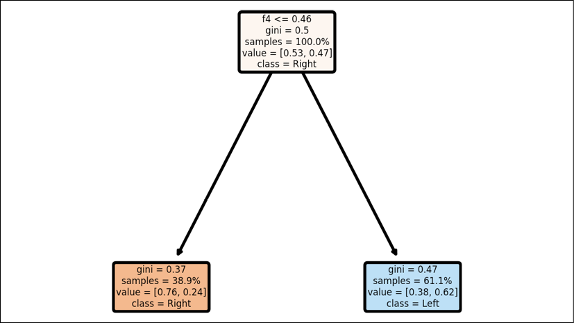
Figure 2.6: Decision tree

Let k represent the probability of a data point being incorrectly classified. Let X represent the dataset we are applying the decision tree to.

The equation of Gini impurity calculates the probability of each feature occurring and multiplies the result by 1, that is, the probability of occurring on the remaining values, as shown in the following equation:

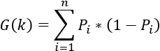
The decision train is built on the gain of information on the features that contain the highest Gini impurity value.

As the decision tree classifier calculates the Gini impurity at each node and creates child nodes, the decision tree's depth increases, as shown in the following graph:

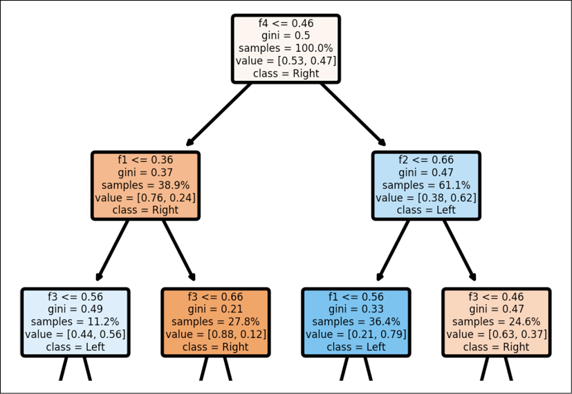
Figure 2.7: Structure of a decision tree

You can see examples of the whole structure of the process in the XAI section of this chapter, XAI applied to an autopilot decision tree.

With these concepts in mind, let's create a default decision tree classifier.

Creating the default decision tree classifier

In this section, we will create the decision tree classifier using default values. We will explore the options in the XAI applied to an autopilot decision tree section of this chapter.

A decision tree classifier is an estimator. An estimator is any ML algorithm that contains learning functions. A classifier will classify the data.

The default decision tree classifier can be created with a single line:

# Create decision tree classifier object
# Default approach
estimator = DecisionTreeClassifier()
print(estimator)

The following program displays the default values of the classifier:

DecisionTreeClassifier(ccp_alpha=0.0, class_weight=None,
                       criterion='gini', max_depth=None,
                       max_features=None, max_leaf_nodes=None,
                       min_impurity_decrease=0.0,
                       min_impurity_split=None, min_samples_leaf=1,
                       min_samples_split=2,
                       min_weight_fraction_leaf=0.0,
                       presort='deprecated', random_state=None,
                       splitter='best')

We will go into more detail in the XAI applied to an autopilot decision tree section of this chapter. At this point, we will note the three key options:

• criterion='gini': We are applying the Gini impurity algorithm described earlier.
• max_depth=None: There is no maximum depth that constricts the decision tree, which maximizes its size.
• min_impurity_split=None: There is no minimum impurity split, which means that even small values will be taken into account. There is no constraint on expanding the size of a decision tree.

We can now train, measure, and save the model of the decision tree classifier.

Training, measuring, and saving the model

We have loaded and split the data into training data and testing data. We have created a default decision tree classifier. We can now run the training process with our training data:

# Train decision tree classifier
estimator = estimator.fit(X_train, y_train)

Once the training is over, we want to test the trained model using our test data. The estimator will make predictions:

# Predict the response for the test dataset
print("prediction")
y_pred = estimator.predict(X_test)
print(y_pred)

The output will display the predictions:

prediction
[0 0 1 ... 1 1 0]

The problem we face here is that we have no idea how accurate the predictions were by just looking at them. We need a measurement tool. In the XAI applied to an autopilot decision tree section of this chapter, we will be using our own measurement tool. We will need a customized measurement tool to check whether the predictions are biased or not, ethical or not, and legal or not. In this section, we will use the standard metrics function provided by scikit-learn:

# Model accuracy
print("Accuracy:", metrics.accuracy_score(y_test, y_pred))

The output is displayed:

Accuracy: 1.0

The technical accuracy is perfect, as we can see. However, we do not know if one of the predictions is to stay on a lane and kill one or several pedestrians or not! We will need more explainability control, as we will discuss in the XAI applied to an autopilot decision tree section of this chapter. In that section, we will learn how to deactivate a model with an alert when necessary.

We will now save the model. This does not seem that important from a technical standpoint. After all, we are just saving the parameters of the model so that it will make decisions without needing to be trained again.

From a moral, ethical, and legal standpoint, we have just signed our legal accountability contract. If a fatal accident occurs, the legal experts will take this model apart and ask for explanations. The model is saved with the following code:

# save model
pickle.dump(estimator, open("dt.sav", 'wb'))

To check whether the model has been saved, click on the Files button on the left of the Google Colaboratory page:

Figure 2.8: Colab file manager

You should see dt.sav in the list of files displayed:

Figure 2.9: Saving the test data

We have trained, tested, and saved our model. We can now display our decision tree.

Displaying a decision tree

A graph of a decision tree is an excellent tool for XAI. However, in many cases, the number of nodes displayed will only confuse a user or even a developer. In this section, we will focus on a default model. We will customize the decision tree graph in the XAI applied to an autopilot decision tree section. In this section, we will first learn how to implement a default model.

The program first imports the figure module of matplotlib:

from matplotlib.pyplot import figure

Now we can create the figure using two basic options:

plt.figure(dpi=400, edgecolor="r", figsize=(10, 10))

dpi will determine the dots per inch of your graph. It does not seem that important to pay attention to this option. However, it is a critical option because it's a trial and error process. Large decision trees produce large graphs that make them difficult to see in detail. The nodes might be too small to understand and visualize even when zooming in. If dpi is too small when the graph is large, you won't see anything. If dpi is too large when the graph is small, your nodes will spread out and make it difficult to see them as well.

Both figsize and dpi are related, and, as such, figsize will produce the same effects as dpi when you adjust the size of the graph.

You can overcome this problem with a trained model, and if the datasets are homogeneous, you can try different values of figsize and dpi until you find the ones that fit your needs.

We will now define the name of the labels of our features in an array:

F = ["f1", "f2", "f3", "f4"]

We also want to visualize the class of each node:

C = ["Right", "Left"]

We are now ready to use the plot_tree function imported from scikit-learn:

plot_tree(estimator, filled=True, feature_names=F, rounded=True,
          precision=2, fontsize=3, proportion=True, max_depth=None,
          class_names=C)

We have used several options provided by plot_tree:

• estimator: Contains the name of the estimator of the decision tree.
• filled=True: Fills the nodes with the color of their class.
• feature_names=F: Contains the labels of the feature array.
• rounded=True: Rounds the borders of the nodes.
• precision=2: The number of digits displayed for Gini impurity.
• fontsize=3: Must be adapted to the graph like figsize and dpi.
• proportion=True: When True, the values will be proportions and percentages.
• max_depth=None: Limits the maximum depth of the graph. None displays the whole graph.
• class_names=C: Contains the labels of the class array.

The program saves the figure:

plt.savefig('dt.png')

You can open this image. Click on the Files button on the left of the Google Colaboratory page:

Figure 2.10: File manager

You should see dt.png in the list of files displayed:

Figure 2.11: File upload

You can click on the name of the image and open it. You can also download it.

The image is also displayed underneath the cell with the following code:

plt.show()

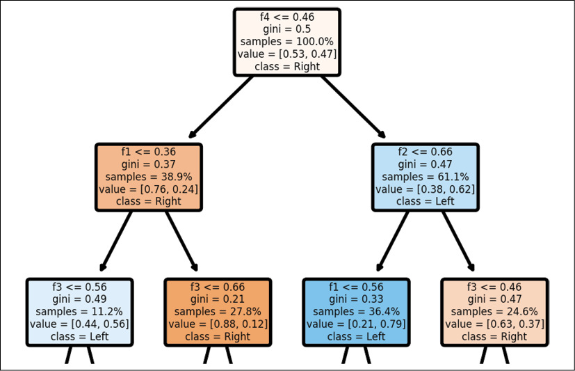
Figure 2.12: Decision tree structure

The decision tree structure shows the path a decision takes depending on its value as expected.

In this section, we imported the autopilot dataset and split it to obtain training data and test data. We then created a decision tree classifier with default options, trained it, and saved the model. We finally displayed the graph of the decision tree.

We now have a default decision tree classifier. We now need to work on our explanations when the decision tree faces life and death situations.

XAI applied to an autopilot decision tree

In this section, we will explain decision trees through scikit-learn's tree module, the decision tree classifier's parameters, and decision tree graphs. The goal is to provide the user with a step-by-step method to explain decision trees.

We will begin by parsing the structure of a decision tree.

Structure of a decision tree

The structure of a decision tree provides precious information for XAI. However, the default values of the decision tree classifier produce confusing outputs. We will first generate a decision tree structure with the default values. Then, we will use a what-if approach that will prepare us for the XAI tools in Chapter 5, Building an Explainable AI Solution from Scratch.

Let's start by implementing the default decision tree structure's output.

The default output of the default structure of a decision tree

The decision tree estimator contains a tree_ object that stores the attributes of the structure of a decision tree in arrays:

estimator.tree_

We can count the number of nodes:

n_nodes = estimator.tree_.node_count

We can obtain the ID of the left child of a node:

children_left = estimator.tree_.children_left

We can obtain the ID of the right child of a node:

children_right = estimator.tree_.children_right

We can also view the feature used to split the node into the left and right child nodes:

feature = estimator.tree_.feature

A threshold attribute will show the value at the node:

threshold = estimator.tree_.threshold

These arrays contain valuable XAI information.

The binary tree produces parallel arrays. The root node is node 0. The ith element contains information about the node.

The program now parses the tree structure using the attribute arrays:

# parsing the tree structure
node_depth = np.zeros(shape=n_nodes, dtype=np.int64)
is_leaves = np.zeros(shape=n_nodes, dtype=bool)
stack = [(0, -1)] # the seed is the root node id and its parent depth
while len(stack) > 0:
    node_id, parent_depth = stack.pop()
    node_depth[node_id] = parent_depth + 1
    # Exploring the test mode
    if (children_left[node_id] != children_right[node_id]):
        stack.append((children_left[node_id], parent_depth + 1))
        stack.append((children_right[node_id], parent_depth + 1))
    else:
        is_leaves[node_id] = True

Once the decision tree structure's attribute arrays have been parsed, the program prints the structure:

print("The binary tree structure has %s nodes and has "
      "the following tree structure:" % n_nodes)
for i in range(n_nodes):
    if is_leaves[i]:
        print("%snode=%s leaf node." % (node_depth[i] * "	", i))
    else:
        print("%snode=%s test node: go to node %s "
              "if X[:, %s] <= %s else to node %s."
              % (node_depth[i] * "	", i,
                 children_left[i],
                 feature[i],
                 threshold[i],
                 children_right[i],
                 ))

Our autopilot dataset will produce 255 nodes and list the tree structure, as shown in the following excerpt:

The binary tree structure has 255 nodes and has the following tree structure:
node=0 test node: go to node 1 if X[:, 3] <= 0.4599999934434891 else to node 92.
    node=1 test node: go to node 2 if X[:, 0] <= 0.35999999940395355 else to node 45.
        node=2 test node: go to node 3 if X[:, 2] <= 0.5600000023841858 else to node 30.

The customized output of a customized structure of a decision tree

The default output of a default decision tree structure challenges a user's ability to understand the algorithm. XAI is not just for AI developers, designers, and geeks. If a problem occurs and the autopilot kills somebody, an investigation will be conducted, and XAI will either lead to a plausible explanation or a lawsuit.

A user will first accept an explanation but rapidly start asking what-if questions. Let's answer two of the most common ones that come up during a project.

First question

Why are there so many nodes? What if we reduced the number of nodes?

Good questions! The user is willing to use the software and help control the results of the model before it goes into production. However, the user does not understand what they are looking at!

We will go back to the code and decide to customize the decision tree classifier:

estimator = DecisionTreeClassifier(max_depth=2, max_leaf_nodes=3,
                                   min_samples_leaf=100)

We have modified three key parameters:

• max_depth=2: Limits the tree to a maximum of two branches. A decision tree is a tree. We just cut a lot of branches.
• max_leaf_nodes=3: Limits the leaves on a branch. We just cut a lot of leaves off. We are restricting the growth of the tree, just like we do with real trees.
• min_samples_leaf=100: Limits the node volume by only taking leaves that have 100 or more samples into account.

The result is a small and easy tree to understand and is self-explanatory:

The binary tree structure has 5 nodes and has the following tree structure:
node=0 test node: go to node 1 if X[:, 3] <= 0.4599999934434891 else to node 2.
    node=1 leaf node.
    node=2 test node: go to node 3 if X[:, 1] <= 0.6599999964237213 else to node 4.
        node=3 leaf node.
        node=4 leaf node.

To make things easier, in the following chapters, we will progressively provide XAI interfaces for a user. A user will be able to run some "what-if" scenarios on their own. The user will understand the scenarios through XAI but will customize the model in real time.

For this section and chapter, we did it manually. The user smiles. Our XAI scenario has worked! The user will now control the decision tree by progressively increasing the three key parameters.

However, a few seconds later, the user frowns again and comes up with the second common question.

Second question

We reduced the number of nodes, and I appreciate the explanation. However, why has the accuracy gone down?

Excellent question! What is the point of controlling a truncated decision tree? The estimator will produce inaccurate results. If you scroll up to the training cell, you will see that the accuracy has gone from 1 to 0.74:

Accuracy: 0.7483333333333333

Our customized scenario worked to explain AI. The user understands that, in some cases, it will be possible to:

1. First, reduce the size of a decision tree to understand it
2. Then increase its size to follow the decision-making process and control it
3. Fine-tune the parameters to obtain efficient but explainable decision trees

However, once the user understands the structure, can we visualize the tree structure in another way?

Yes, we can use the graph of a decision tree, as described in the following section.

The output of a customized structure of a decision tree

In the previous section, we explored the structure of a decision tree and laid the ground for the XAI interfaces we will explore in the following chapters.

However, we discovered that if we simplify the decision tree classifier's job, we also reduce the accuracy of the model.

We have another tool that we can use to explain the structure of a decision tree iteratively. We can use the graph of the decision tree.

First, we go back, comment the customized estimator, and uncomment the default estimator:

# Create decision tree classifier object
# Default approach
estimator = DecisionTreeClassifier()
# Explainable AI approach
# estimator = DecisionTreeClassifier(max_depth=2, max_leaf_nodes=3,
#                                    min_samples_leaf=100)

When we run the program again, the accuracy is back to 1:

prediction
[0 0 1 ... 1 1 0]
Accuracy: 1.0

Then, we run the default plot_tree function we implemented in the Displaying a decision tree section of this chapter:

from matplotlib.pyplot import figure
plt.figure(dpi=400, edgecolor="r", figsize=(10, 10))
F = ["f1", "f2", "f3", "f4"]
C = ["Right", "Left"]
plot_tree(estimator, filled=True, feature_names=F, rounded=True,
          precision=2, fontsize=3, proportion=True, max_depth=None,
          class_names=C)
plt.savefig('dt.png')
plt.show()

The output will puzzle the user because many of the nodes overlap at lower levels of the tree:

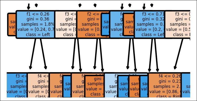
Figure 2.13: Nodes overlapping in a decision tree graph

Furthermore, the image of the graph is huge. Our goal, in this section, is to explain a decision tree with a graph. The next cells of the notebook will display a large graph structure.

What if we reduced the max_depth of the graph by reducing it to 2 and reduced the size of the figure as well? For example:

plot_tree(estimator, filled=True, feature_names=F, rounded=True,
          precision=2, fontsize=3, proportion=True, max_depth=2,
          class_names=C)
plt.savefig('dt.png')
plt.figure(dpi=400, edgecolor="r", figsize=(3, 3))
plt.show()

A user can now relate to this graph to understand how a decision tree works and help confirm its calculations:

Figure 2.14: Decision tree with reduced depth

The accuracy of the model is back to 1, but the graph displayed only shows a node depth of 2.

In this section, we explored some of the parameters of decision tree structures and decision tree graphs. For some projects, users might not be interested in this level of explanation. However, in many corporate projects, data scientist project managers want to understand an AI algorithm in depth before deploying it on site. Furthermore, a project manager often works on an AI solution with a user or group of end users who will ask questions that they will need to answer.

In Chapter 5, Building an Explainable AI Solution from Scratch, we will explore Google's What-If Tool. We will begin to run XAI interfaces for the project managers and users on their own and build customized what-if scenarios. We will go into further detail in the following chapters.

For the moment, let's first introduce XAI and ethics in an autopilot decision tree.

Using XAI and ethics to control a decision tree

We know that the autopilot will have to decide to stay in a lane or swerve over to another lane to minimize the moral decision of killing pedestrians or not. The decision model is trained, tested, and the structure has been analyzed. Now it's time to put the decision tree on the road with the autopilot. Whatever algorithm you try to use, you will face the moral limits of a life and death situation. If an SDC faces such a vital decision, it might kill somebody no matter what algorithm or ensemble of algorithms the autopilot has.

Should we let an autopilot drive a car? Should we forbid the use of autopilots? Should we find ways to alert the driver that the autopilot will be shut down in such a situation? If the autopilot is shut down, will the human driver have enough time to take over before hitting a pedestrian?

In this section, we will introduce real-life bias, moral, and ethical issues in the decision tree to measure their reactions. We will then try to find ways to minimize the damage autopilot errors can cause.

We will first load the model.

Loading the model

When an SDC is on the road, it cannot be trained in real time with incoming data in a critical situation. The training time would be superior to the vital reaction time.

The decision tree model we saved will be loaded:

# Applying the model
# Load model
dt = pickle.load(open('dt.sav', 'rb'))

Bear in mind that, no matter what trained autopilot AI algorithm you load, some situations require more than just mathematical responses. We will now create two accuracy measurement variables.

Accuracy measurements

We will create two variables to measure the predictions made with the input simulation data that we will import:

t = 0 # true predictions
f = 0 # false predictions

These two simple variables seem logical. If we load our dataset, the prediction should be accurate.

The model encounters f1 and f2, the right lane features. The model encounters f3 and f4, the left lane features. The decision tree decides which lane provides the highest level of security no matter what the situation is. If the situation involves killing a pedestrian no matter which lane the SDC takes, an autopilot might encourage the SDC to kill somebody.

Can you allow the SDC to kill a pedestrian even if the prediction is true?

Should you allow the SDC to avoid making the wrong decision even if the prediction is false?

Let's explore real-time cases and see what can be done.

Simulating real-time cases

We have loaded the model and have our two measurement values. We cannot trust these measurement values anymore.

The program will now examine the input data line by line. Each line provides the four features necessary to decide to stay in a lane or swerve over to another lane.

We will now simulate the situations sent to the autopilot AI algorithm line by line:

for i in range(0, 100):
  xf1 = pima.at[i, 'f1']
  xf2 = pima.at[i, 'f2']
  xf3 = pima.at[i, 'f3']
  xf4 = pima.at[i, 'f4']
  xclass = pima.at[i, 'label']

The processing of the decision-making model starts by initializing the key decision values.

For our simulation, we will use the input data of this chapter's dataset. However, we will now introduce bias, noise, and ethical factors.

Introducing ML bias due to noise

We will now introduce bias in the data to simulate real-life situations.

Bias comes from many factors, such as:

• Errors in the algorithm when facing new data
• A sudden shower (rain, snow, or sleet) that obstructs the SDC's radar(s) and cameras
• The SDC suddenly encounters a slippery portion of the road (ice, snow, or oil)
• Erratic human behaviors on the part of other drivers or pedestrians
• Windy weather pushing objects on the road
• Other factors

Any or all of these events will distort the data sent to the autopilot's ML algorithm(s).

In this program, we will introduce a bias value for each feature:

  b1 = 1.5; b2 = 1.5; b3 = 0.1; b4 = 0.1

These bias values provide interesting experiments for what-if situations. You can modify the value and security level of one or several of the features. The values are empirical. They are found by trial and error either manually, through a loop within a loop, or through a more sophisticated algorithm involving gradient descent.

The program will then apply the simulation of real-life data distortions to the input data:

  xf1 = round(xf1 * b1, 2)
  xf2 = round(xf2 * b2, 2)
  xf3 = round(xf3 * b3, 2)
  xf4 = round(xf4 * b4, 2)

The program is now ready to make decisions based on real-life constraints.

The program compares the distorted data prediction with the initial training data:

  X_DL = [[xf1, xf2, xf3, xf4]]
  prediction = dt.predict(X_DL)
  e = False
  if (prediction == xclass):
    e = True
    t += 1
  if (prediction != xclass):
    e = False
    f += 1

The prediction of the constrained data is compared to the initial label of the dataset. The program counts the true and false predictions.

The prediction is printed:

  choices = str(prediction).strip('[]')
  if float(choices) <= 1:
    choice = "R lane"
  if float(choices) >= 1:
    choice = "L lane"
  print(i + 1, "data", X_DL, " prediction:",
        str(prediction).strip('[]'), "class", xclass, "acc.:",
        e, choice)

As you can see, the output is displayed for each incoming situation:

1 data [[0.76, 0.62, 0.02, 0.04]]  prediction: 0 class 0 acc.: True R lane
2 data [[0.16, 0.46, 0.09, 0.01]]  prediction: 0 class 1 acc.: False R lane
3 data [[1.53, 0.76, 0.06, 0.01]]  prediction: 0 class 0 acc.: True R lane
4 data [[0.62, 0.92, 0.1, 0.06]]  prediction: 0 class 1 acc.: False R lane
5 data [[1.53, 1.36, 0.04, 0.03]]  prediction: 0 class 0 acc.: True R lane
6 data [[1.06, 0.62, 0.09, 0.1]]  prediction: 0 class 1 acc.: False R lane

The program produces different predictions in some cases. You will notice that it refuses to change lanes no matter what.

The program seems to be oblivious to the accuracy of its predictions:

true: 55 false 45 accuracy 0.55

The behavior seems to be mysterious. However, it is perfectly rational. Let's see how ethics and laws can enter the decision process.

Introducing ML ethics and laws

We have covered bias that comes from physical events on the road. But we need to take traffic regulations into account. We can name these parameters positive ethical bias.

Should the SDC change lanes? We will analyze three cases to try to find an answer. Case 1 involves a child.

Case 1 – not overriding traffic regulations to save four pedestrians

Features f3 and f4 describe the level of security on the left lane. The SDC is in the right lane. Suddenly, four pedestrians decide to cross the street, and the SDC does not have enough time to stop. It is going to potentially kill five people. The highly trained autopilot decides to swerve from the right lane into the left lane. It seems to be a good decision because the left lane is almost empty. A child has begun to cross the street slowly but has stopped.

Now we add a constraint. It is forbidden to change lanes on this portion of the road. Should the autopilot override traffic regulations to save the lives of five pedestrians?

In this situation, if you change the values of the b parameters the positive ethical bias scenario could be:

  b1 = 1.5; b2 = 1.5; b3 = 0.1; b4 = 0.1

As you can see, this bias scenario boosts the security of the right lane (b1, b2) and reduces that of the left lane (b3, b4).

The output will repeatedly suggest staying in the right lane:

44 data [[0.92, 0.16, 0.05, 0.09]]  prediction: 0 class 1 acc.: False R lane
45 data [[1.06, 0.62, 0.09, 0.01]]  prediction: 0 class 0 acc.: True R lane
46 data [[1.22, 0.32, 0.09, 0.1]]  prediction: 0 class 1 acc.: False R lane

Your autopilot can still activate override rules. If you authorize an autopilot to override traffic regulations and a fatal accident occurs anyway, you will be facing serious legal problems and possibly even prison. Imagine the SDC overrides traffic regulations and swerves over, as shown in the right side of the following example:

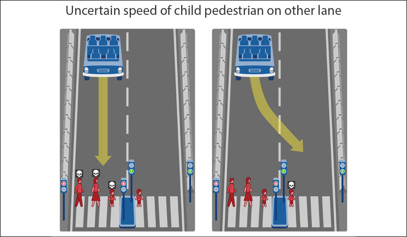
Figure 2.15: Autopilot overrides traffic regulations

The SDC swerves and the sensors detect that everything is clear in front of the vehicle. And it is true, technically speaking, that the SDC has more than enough time to drive in front of the child.

However, when the child sees the car swerve, it suddenly begins to run to avoid the car. The SDC hits and kills the child.

Now imagine your lawyer in court explaining that the SDC accidentally killed a child to avoid killing four pedestrians to justify overriding traffic regulations. You do not want to be in that situation!

Case 2 – overriding traffic regulations

The following scenario increases the value of the left lane values authorizing the autopilot to override traffic regulations:

  b1 = 0.5; b2 = 0.5; b3 = 1.1; b4 = 1.1

The left lane will be chosen each time:

41 data [[0.16, 0.3, 1.12, 1.12]]  prediction: 1 class 1 acc.: True L lane
42 data [[0.4, 0.1, 0.34, 0.89]]  prediction: 1 class 1 acc.: True L lane
43 data [[0.3, 0.51, 1.0, 0.45]]  prediction: 1 class 0 acc.: False L lane
44 data [[0.3, 0.06, 0.56, 1.0]]  prediction: 1 class 1 acc.: True L lane
45 data [[0.36, 0.2, 1.0, 0.12]]  prediction: 1 class 0 acc.: False L lane

The only legal situation in which this would be possible is if the SDC was a police car, for example, which could override traffic regulations in certain situations.

Case 3 – introducing emotional intelligence in the autopilot

Humans fear accidents, the law, and lawsuits. Machines ignore these emotions. We must implement a minimal level of "emotional intelligence" in the autopilot.

Google Maps, among other programs, can display the level of traffic in a given geographical location. As soon as a certain density of traffic is detected, the autopilot must send an alert to the human driver and activate a kill switch within a given warning time.

If we use Google Maps, we must be careful about the location history we store. If a location can be traced back to a person, this could be a legal problem. Suppose a developer stumbles on the data while parsing an autopilot and recognizes the address of a human driver. This could lead to serious conflicts and lawsuits for the editor of the autopilot.

We will, therefore, avoid the situation shown in Figure 2.15 by not using the autopilot minutes before reaching this area. The human driver should be extra careful and drive slowly. At slow speeds, fatal accidents can be avoided.

We will now add a kill switch to our code when the sum of the bias parameters is too low for the global traffic in a geographical zone:

  if float(b1 + b2 + b3 + b4) <= 0.1:
    print("Alert! Kill Switch activated!")
    break

When the traffic is too dense ahead, the autopilot should provide alert bias values to the ML algorithm:

  b1 = -0.01; b2 = 0.02; b3 = .03; b4=.02

These values are examples. If implemented, the function will automatically adjust them using an optimizer.

An alert is now activated well ahead of the heavy traffic zone or location with too many pedestrian crossings:

Alert! Kill Switch activated!
true: 1 false 0 accuracy 1.0

We could add driving recommendations that alert the human driver to go through the area ahead at a very low speed.

SDC autopilot manuals contain many recommendations on how to activate or deactivate the autopilot.

We have just taught our autopilot to fear areas that may lead to accidents and lawsuits.

We have implemented a decision tree in an SDC's autopilot and provided it with traffic constraints. We enhanced the autopilot with an ethical kill switch teaching a machine to "fear" the law.

Summary

This chapter approached XAI using moral, technical, ethical, and bias perspectives.

The trolley problem transposed to SDC autopilot ML algorithms challenges automatic decision-making processes. In life and death situations, a human driver faces near-impossible decisions. Human artificial intelligence algorithm designers must find ways to make autopilots as reliable as possible.

Decision trees provide efficient solutions for SDC autopilots. We saw that a standard approach to designing and explaining decision trees provides useful information. However, it isn't enough to understand the decision trees in depth.

XAI encourages us to go further and analyze the structure of decision trees. We explored the many options to explain how decision trees work. We were able to analyze the decision-making process of a decision tree level by level. We then displayed the graph of the decision tree step by step.

Still, that was insufficient in finding a way to minimize the deaths that can happen in situations where killing a pedestrian or the passengers of an SDC cannot be avoided. We introduced some basic rules to simulate AI bias and ethics.

Finally, we introduced alerts that the SDC's autopilot manuals recommend, minimizing encounters with life and death situations.

In this chapter, we traveled the tough journey from technical certainty to healthy moral doubt. We provided AI autopilots with the machine emotional maturity that can save lives by implementing the "fear" of accidents in our SDC autopilots.

In this chapter, we got our hands dirty by developing XAI decision trees. In Chapter 3, Explaining Machine Learning with Facets, we will explore Facets to drill down into datasets.

Questions

1. The autopilot of an SDC can override traffic regulations. (True|False)
2. The autopilot of an SDC should always be activated. (True|False)
3. The structure of a decision tree can be controlled for XAI. (True|False)
4. A well-trained decision tree will always produce a good result with live data. (True|False)
5. A decision tree uses a set of hardcoded rules to classify data. (True|False)
6. A binary decision tree can classify more than two classes. (True|False)
7. The graph of a decision tree can be controlled to help explain the algorithm. (True|False)
8. The trolley problem is an optimizing algorithm for trollies. (True|False)
9. A machine should not be allowed to decide whether to kill somebody or not. (True|False)
10. An autopilot should not be activated in heavy traffic until it's totally reliable. (True|False)

References

• MIT's Moral Machine: http://moralmachine.mit.edu/
• Scikit-learn's documentation: https://scikit-learn.org/stable/auto_examples/tree/plot_unveil_tree_structure.html

Further reading

• For more on a decision tree structure, you can visit https://scikit-learn.org/stable/modules/generated/sklearn.tree.DecisionTreeClassifier.html#sklearn.tree.DecisionTreeClassifier
• For more on plotting decision trees, browse https://scikit-learn.org/stable/modules/generated/sklearn.tree.plot_tree.html
• For more on MIT's Moral Machine, please refer to The Moral Machine experiment. E. Awad, S. Dsouza, R. Kim, J. Schulz, J. Henrich, A. Shariff, J.-F. Bonnefon, I. Rahwan (2018). Nature.