
11
Anchors XAI
The explainable AI (XAI) tools we have explored up to now are model-agnostic. They can be applied to any machine learning (ML) model. The XAI tools we implemented come from solid mathematical theory and Python modules. In Chapter 8, Local Interpretable Model-Agnostic Explanations (LIME), we even ran several ML models to prove that LIME, for example, was model-agnostic.
We can represent model-agnostic (ma) tools as a function of ML(x) algorithms in which ma(x) -> Explanations. You can read the function as a model-agnostic tool that will generate explanations for any ML model.
However, the opposite is not true! Explanations(x) -> ma is false. You can read the function as an explanation of any ML model that can be obtained by any model-agnostic tool x. A model-agnostic XAI tool can technically work with an ML model x, but the results may not be satisfactory.
We can even say that an XAI tool might work with an ML algorithm and that ma(x) is true. But if we change the dataset and goals of an AI project, the same ma(x) will be inaccurate. We must add the dataset d to our analysis. ma(x(d)) -> Explanations now takes the dataset into account. A dataset d that contains very complex images will not be as simple to explain as a dataset containing simple images.
We think we can choose an XAI tool by first analyzing the dataset. But there is still another problem we need to solve. A "simple" dataset containing words might also contain so many words that we may find that in the true and false predictions, it confuses the XAI tool! We now need to add the instance i of a dataset to our analysis of XAI tools, expressed as ma(x(d(i))) -> Explanations.
In Chapter 8, Local Interpretable Model-Agnostic Explanations (LIME), we saw that LIME focuses on ma(x(d(i))), a specific instance of a dataset, to explain the output of the model by examining the vicinity, the features around the core of the prediction. LIME took us down to one prediction and its local interpretable environment. We might think that there is nothing left to do.
However, LIME (from Ribeiro, Singh, and Guestrin) found that though their tool could be locally accurate, some of the explanatory features did not influence the prediction as planned. LIME would work with some datasets and not others.
Ribeiro, Singh, and Guestrin have introduced high-precision rules, anchors, to increase the efficiency of the explanation of a prediction. The explanatory function now becomes ma(x(d(i))) -> high-precision anchor explanations using rules and thresholds to explain a prediction. Anchors take us deep into the core of XAI.
In this chapter, we will begin by examining anchor AI explanations through examples. We will use text examples to define anchors, which are high-precision rules.
We will then build a Python program that explains ImageNet images with anchors.
By the end of the chapter, you will have reached the core of XAI.
This chapter covers the following topics:
- High-precision rules – anchors
- Anchors in text classification
- An example of text classification with LIME and anchors
- The productivity of anchors
- The limits of LIME in some cases
- The limits of anchors
- A Python program to explain ImageNet images with anchors
- Implementing an anchors explanation function in Python
- Visualizing anchors in an image
- Visualizing all the superpixels of an image
Our first step will be to explore the anchors explanation method with examples.
Anchors AI explanations
Anchors are high-precision model-agnostic explanations. An anchor explanation is a rule or a set of rules. The rule(s) will anchor the explanations locally. Changes to the rest of the feature values will not matter anymore for a specific instance.
The best way to understand anchors is through examples. We will define anchor rules through two examples: predicting income and classifying newsgroup discussions.
We will begin with an income prediction model.
Predicting income
In Chapter 5, Building an Explainable AI Solution from Scratch, we built a solution that could predict income levels.
We found a ground truth that has a strong influence on income: age and level of education are critical features that determine the income level of a person.
The first key feature we found was that age is a key factor when predicting the income of a person, as shown in the following chart:
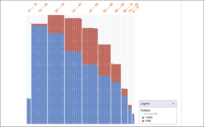
Figure 11.1: Income by age
The red (shown in the color image) values form the top section of each bar and represent people with a level of income >50K. The blue (shown in the color image) values form the bottom sections of the bars and represent people with a level of income <=50K.
Universal principles clearly appear:
- A ten-year-old person earns less than a person that is 30 years old
- A person that is over 70 years old is more likely than not to be retired and have a lower income than a person that is 40 years old
- The income curve increases from childhood to adulthood, reaches a peak, and then goes slowly down with age
The feature we found was the level of education. When we binned the age categories and included the level of education, we obtained a realistic income chart:
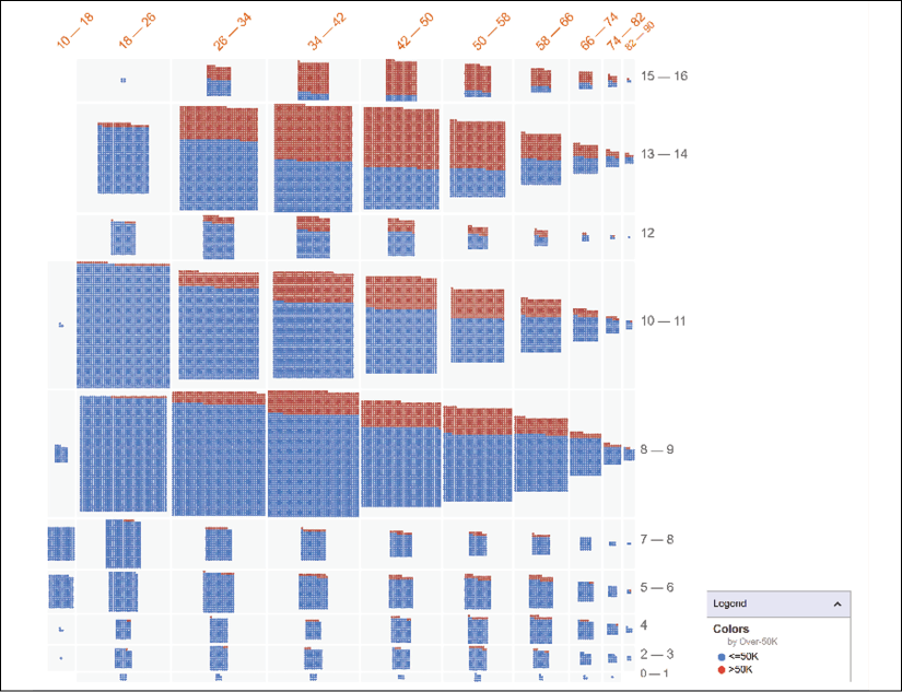
Figure 11.2: Income by age and number of years of education
We conclude that several additional universal principles appear:
- The longer a person studies, the more that person will earn
- The longer a person gains experience in work, the more that person will earn
- Learning can be acquired through experience
- After a few years of experience, a person with higher education will make more
- The age factor is intensified by education and experience, which explains why the higher-income portion of the bars increases in a significant way starting at age 30, for those having between 13 and 17 years of education for example
Let's now suppose that the anchors explanations tool used the same dataset as we did in Chapter 5, Building an Explainable AI Solution from Scratch. We used a version of the U.S. census dataset that was transformed into an international legal and ethical dataset. The idea was to predict whether a person earned more or less than 50K.
The anchor explainer would probably come up with the following anchor explanation:
IF Country = United States AND 34 <= Age <= 42
AND Number of years of education >= 14
THEN PREDICT Income > USD50K
The anchor explanation is very strongly "anchored." It will most likely remain constant even if other values are changed. Naturally, this explanation will not be 100% true in every instance, but it is highly precise and efficient.
The beauty of anchor explanations is that they are high-precision explanations that we can all understand.
The wonder of anchor explanations is that they are produced automatically!
Let's now see why anchors can produce better results than LIME in some cases.
Classifying newsgroup discussions
In Chapter 8, Local Interpretable Model-Agnostic Explanations (LIME), we implemented LIME to classify newsgroup discussions into two categories: "electronics" and "space."
We built a LIME explainer that produced a visual explanation for each instance. Let's examine the following LIME explanation, for instance:
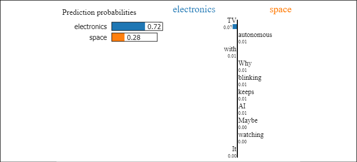
Figure 11.3: LIME explanation
We can see that the prediction was electronics based on the left side of the explanation:
- TV
- with
- It
However, the features for space include the following:
- watching
- Why
- keeps
We can see that the word "TV" can guarantee a prediction for electronics, for example.
In another instance, if we see "watching" and "TV" on the electronics side, it will make the prediction even more probable.
We can now imagine a highly precise anchor explanation:
IF feature x = "TV"
AND feature y = "watching"
THEN PREDICT category = electronics
We can only admire the way anchor explanations were designed to provide such clear and precise explanations.
In this section, we went through anchors for text classification. If you wish to further explore text classification with anchors, you can consult the following example applied to movie reviews: https://docs.seldon.io/projects/alibi/en/stable/examples/anchor_text_movie.html
You could then compare the method used with anchors with the SHAP program we created for movie reviews in Chapter 4, Microsoft Azure Machine Learning Model Interpretability with SHAP.
We will now build a Python program to explain ImageNet images with anchors. It will be interesting to discover how anchor explanations of images are visualized.
Anchor explanations for ImageNet
In this section, we will build a Python Alibi program that will produce anchors for images. Alibi is a library that contains several XAI resources.
We will use images from ImageNet to run the explainer.
We will build the program in the following order:
- Installing Alibi and importing the modules
- Loading an
InceptionV3model - Downloading an image to explain
- Processing the image and making predictions
- Creating the anchor image explainer and displaying the visual explanations
Let's first install Alibi and import the modules.
Installing Alibi and importing the modules
To get started, open the Image_XAI_Anchor.ipynb notebook for this chapter. This notebook is in the chapter directory of this book.
We will first install Alibi as follows:
# @title Install Alibi
try:
  import alibi
except:
  !pip install alibi
If Alibi is installed, the program will continue. However, when Colaboratory restarts, some libraries and variables are lost. In this case, the program will install Alibi.
We will now install the modules for the program.
We will first import the necessary modules for this program. We will then import the data and display a sample.
The program will import two types of modules: TensorFlow modules and modules that Alibi will use to display the explainer's output.
# @title Importing modules
import tensorflow as tf
# tf.logging.set_verbosity(tf.logging.ERROR) # suppress deprecation
                                             # messages
import matplotlib
%matplotlib inline
import matplotlib.pyplot as plt
import numpy as np
from tensorflow.keras.applications.inception_v3 import InceptionV3, preprocess_input, decode_predictions
from alibi.datasets import fetch_imagenet
from alibi.explainers import AnchorImage
Let's now load the InceptionV3 model.
Loading an InceptionV3 model
In this section, we will load a pretrained InceptionV3 model. InceptionV3 is an image recognition model. It produces acceptable results on the ImageNet dataset.
By acceptable, I mean that XAI tools, as well as AI models, are not dataset-agnostic, as we will see in the Building the anchor image explainer subsection in this section.
The model contains image processing layers such as convolutions, pooling, dropouts, and dense layers.
The model is loaded with the following code:
# @title Load InceptionV3 model pretrained on ImageNet
model = InceptionV3(weights='imagenet')
Let's now download the images to train on and explain them.
Downloading an image
ImageNet contains 1,000 classes of labeled images that you can consult at https://gist.github.com/yrevar/942d3a0ac09ec9e5eb3a.
The list contains a variety of categories, as shown in the following excerpt:
1: 'goldfish, Carassius auratus',
2: 'great white shark, white shark, man-eater, man-eating shark, Carcharodon carcharias',
3: 'tiger shark, Galeocerdo cuvieri',
4: 'hammerhead, hammerhead shark',
5: 'electric ray, crampfish, numbfish, torpedo',
6: 'stingray',
7: 'cock',
8: 'hen',
9: 'ostrich, Struthio camelus',
10: 'brambling, Fringilla montifringilla',
Alibi has focused on a limited number of ImageNet categories that are listed in datatsets.py, an Alibi backend program for downloading ImageNet images:
mapping = {'Persian cat': 'n02123394',
           'volcano': 'n09472597',
           'strawberry': 'n07745940',
           'centipede': 'n01784675',
           'jellyfish': 'n01910747'}
A form was added to the program to choose a category of images to explain:

Figure 11.4: Selecting a category
Once a category is selected, the program sets the image shape. Then it retrieves the data and the corresponding labels of the images:
# @title Download image form ImageNet
category = 'Persian cat' # @param ["Persian cat", "volcano",
#                                  "strawberry", "centipede",
#                                  "jellyfish"]
image_shape = (299, 299, 3)
data, labels = fetch_imagenet(category, nb_images=25,
                              target_size=image_shape[:2],
                              seed=2, return_X_y=True)
print('Images shape: {}'.format(data.shape))
The images are downloaded and ready to be processed to make predictions.
Processing the image and making predictions
The program now processes the images and makes predictions with the pretrained InceptionV3 model:
# @title Process image and make predictions
images = preprocess_input(data)
preds = model.predict(images)
label = decode_predictions(preds, top=3)
print(label[0])
# @title Define prediction model
predict_fn = lambda x: model.predict(x)
We are now all set. We imported, processed, and made predictions on the images. We can now build the anchor image explainer and visualize the explanations.
Building the anchor image explainer
In this section, we will build the anchor image explainer and display the visual explanations.
The Alibi anchor image explainer has scikit-learn's built-in segmentation methods. In this notebook, the slic segmentation function is selected:
# @title Initialize anchor image explainer
segmentation_fn = 'slic'
kwargs = {'n_segments': 15, 'compactness': 20, 'sigma': .5}
explainer = AnchorImage(predict_fn, image_shape,
                        segmentation_fn=segmentation_fn,
                        segmentation_kwargs=kwargs,
                        images_background=None)
slic uses k-means clustering in color space to segment an image. Alibi has built the function in its module. However, the key parameters are standard in the kwargs argument:
n_segmentsrepresents the number of labels in the segmented output image.compactnesswill produce superpixel shapes by balancing color proximity and space proximity. The explainer will use these superpixels.sigmais the size of the Gaussian smoothing kernel. The kernel will preprocess each dimension of the image.
The explainer is initialized with the variables we prepared up to this point:
predict_fn = model.predict(x)image_shape = (299, 299, 3)segmentation_fn = 'slic'segmentation_kwargs = kwargs(images_background=None)is not initialized at this point
The explainer is now ready to produce outputs.
The program will now display the image:
i = 0
plt.imshow(data[i]);
The output displays the image:
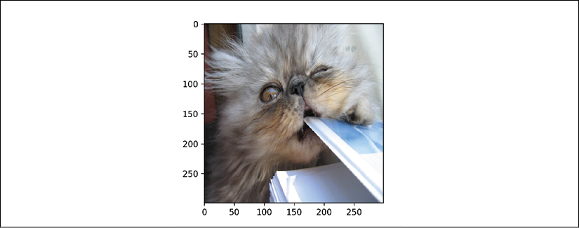
Figure 11.5: Persian cat
You can change i = 0 to another image to display within the range of nb_images=25 defined in the download function of this program. You can also increase the value of nb_images if you wish to explore more visual anchors.
The program now produces the anchor explanation:
# @title Anchor explanation
image = images[i]
np.random.seed(0)
explanation = explainer.explain(image, threshold=.95,
                                p_sample=.5, tau=0.25)
The parameters of explanation are as follows:
Imageisimages[i].threshold=.95is the minimum fraction of samples to take into account.p_sample=.5is the portion of superpixels that are changed. They can be averaged, for example.tau=0.25is the convergence level. If the value is high, convergence will be reached faster but with fewer anchor constraints.
The program now displays the superpixels in the anchor:
# @title Superpixels in the anchor
plt.imshow(explanation.anchor);
The output is a visual explanation that contains the anchors:
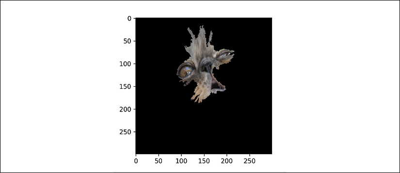
Figure 11.6: Anchors of a Persian cat
We have a visual anchor explanation.
The program will also display all the superpixels (there may be slight variations of color) so that we can see the segments in the image:
# @title All superpixels
plt.imshow(explanation.segments);
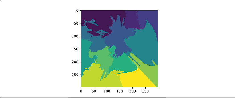
Figure 11.7: Displaying all the superpixels
We have implemented the anchor explanation process. Let's visualize more explanations.
Explaining other categories
Go back to the category selection form and choose strawberry from the dropdown list:

Figure 11.8: Selecting a category
Then run the program, and you will visualize the superpixels and the anchor. The first image is the original image, and the second one shows the anchor:
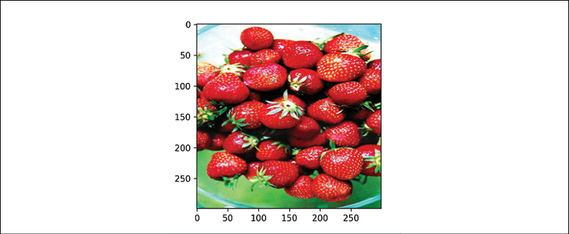
Figure 11.9: Original image of strawberries
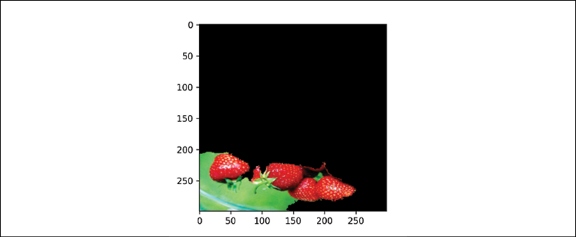
Figure 11.10: Anchor explanations
Now go back to the category form and select centipede:

Figure 11.11: Selecting a category
This image has a lot of contrast, which is interesting. The first image is the original image, while the second one shows the anchor:
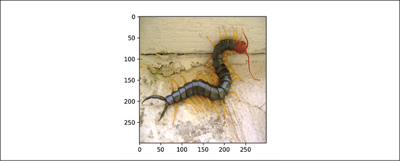
Figure 11.12: Our centipede image
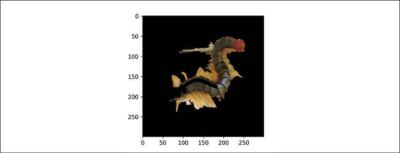
Figure 11.13: Anchor explanations
You can select other images within the categories to visualize anchors from different perspectives depending on the image.
As always, there are limitations to this XAI tool, as we will see now.
Other images and difficulties
The categories we have chosen up to now lead to good visual anchor explanations.
However, if you select jellyfish, the superpixels may be detected, and maybe the anchor too. The first image is the original one.
But the explanation with the superpixels in the anchor is not displayed, as you can see in the second image that follows:
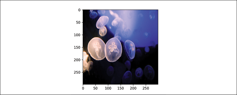
Figure 11.14: Jellyfish
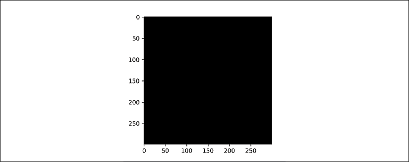
Figure 11.15: Anchor explanation failed
This black image requires an investigation. It could be a limit of the explainer, it could be that the parameters need to be changed through trial and error, it could be the choice of image, or a problem with InceptionV3.
In any case, in this notebook, when I tried the categories, the anchor explanation statuses were as follows:
- persian cat = OK
- jellyfish = failed
- volcano = failed
- strawberry = OK
- centipede = OK
In this section, we confirmed that anchors can also be applied to images. We built a Python program and produced anchor explanations for ImageNet images. We also discovered the natural limitations of any XAI tool.
These limitations should encourage us to get involved in open source XAI tool projects to help improve the programs. It also shows that we might need to change XAI tools when we reach the limits of a specific XAI method.
Summary
In this chapter, we explored the boundaries of XAI tools. We found that an XAI tool, though model-agnostic, is not dataset-agnostic! An XAI tool might work well for text classification and not for images. An XAI tool might even work with some text classification datasets and not others.
We first described how a model-agnostic XAI tool cannot be dataset-agnostic. We used the knowledge gathered in the previous chapters to explain the limitations of an XAI tool when it reaches the boundaries of a prediction.
We saw how the interception function developed in Chapter 4, Microsoft Azure Machine Learning Model Interpretability with SHAP, introduced samples containing pseudo-anchors in the IMDb dataset. SHAP then interpreted these values as anchors and provided a SHAP explanation.
We transformed the prediction process of the model built in Chapter 6, AI Fairness with Google's What-If Tool (WIT), into an anchor explanation.
We also used the LIME explanations from Chapter 8, Local Interpretable Model-Agnostic Explanations (LIME), to illustrate the limits of LIME and how to improve the explanation with anchors.
Finally, we ran a program in Python to explain images with anchors. The anchor explainer detected superpixels in an image to produce explanations.
Anchor explanations can thus be sets of rules with thresholds that apply to text classification as well as image-based predictions.
In the next chapter, Cognitive XAI, we will continue to explore how to explain AI with rules. We will see how to build human-made rules to explain AI.
Questions
- LIME explanations are global rules. (True|False)
- LIME explains a prediction locally. (True|False)
- LIME is efficient on all datasets. (True|False)
- Anchors detect the ML model used to make a prediction. (True|False)
- Anchors detect the parameters of an ML model. (True|False)
- Anchors are high-precision rules. (True|False)
- High-precision rules explain how a prediction was reached. (True|False)
- Anchors do not apply to images. (True|False)
- Anchors can display superpixels on an image. (True|False)
- A model-agnostic XAI tool can run on many ML models. However, not every ML model is compatible with an XAI tool for specific applications. (True|False)
References
- The reference code repositories for anchors can be found at the following links:
- https://github.com/SeldonIO/alibi/blob/524d786c81735ed90da2d2c68851c1145fa1b595/examples/anchor_image_imagenet.ipynb
- https://github.com/SeldonIO/alibi/tree/524d786c81735ed90da2d2c68851c1145fa1b595
The reference documentation for anchors can be found at https://docs.seldon.io/projects/alibi/en/stable/methods/Anchors.html
- The reference documentation for scikit-learn segmentation methods can be found at https://scikit-image.org/docs/dev/api/skimage.segmentation.html
Further reading
- For more on anchors, see the paper Anchors: High-Precision Model-Agnostic Explanations by Ribeiro, Singh, and Guestrin, available at https://homes.cs.washington.edu/~marcotcr/aaai18.pdf
- For more on Alibi, see the documentation at https://docs.seldon.io/projects/alibi/en/stable/index.html
- For more on the
InceptionV3model, check out the following two links: