
12
Cognitive XAI
Machines compute, humans construe. Humans interpret what they perceive. AI makes fabulous mathematical representations of the world. Humans conceptualize ideas. Machines still lack consciousness. Humans have self-awareness. Machines can outperform humans in many fields. Humans can reduce machines to dust with ethics. Machine intelligence takes raw data, makes sense of it, and will produce predictions. Humans take raw data, interpret it, and make careful decisions to avoid conflicts.
Everything goes well as long as these two forms of intelligence work converge. When they collide, the machine, or rather its owner, will have a tremendous price to pay. In the United States, punitive damages award mind-blowing levels of financial compensation to plaintiffs well beyond the actual damage caused by a defendant. In the European Union, the General Data Protection Regulation (GDPR) summons a corporation to explain an automatic process with human intervention. The sanctions applied can reach 4% of the global revenue of a cloud giant.
A human court of law will construe (interpret) machine intelligence damage to an individual as a severe violation of the law. We can avoid these situations by helping a human to understand AI through XAI.
We have explored a whole new world of AI through explainable AI tools in this book. This wide range of tools can explain AI. SHAP provides the marginal contribution of a feature. Facets can display data in an interpretable manner. We can make simulations with WIT. The contrastive explanation method's (CEM) unconditionality shows how far one prediction is from another. LIME explains a prediction locally. Contrastive explanations show why the absence or presence of a feature is critical. Anchors offer the extraordinary tool of context, the connection between words.
Cognitive explanations cannot replace the power of the XAI tools we have explored, but they will help a human understand XAI's machine reasoning.
Cognitive human-oriented explanations will bridge the gap between explanations, and initiate the moment when somebody says, "Right, now I get it! Thanks for the explanation."
We will begin the chapter by defining cognitive rule-based explanations. We will create a cognitive Python application to help a user understand the SHAP program we built in Chapter 4, Microsoft Azure Machine Learning Model Interpretability with SHAP.
Then, we will use our human-centered reasoning power to help a human understand and improve the LIME-WIT project in Chapter 8, Local Interpretable Model-Agnostic Explanations (LIME).
Finally, we will add human cognitive reasoning to improve the use of the vectorizer for the CEM project in Chapter 9, The Counterfactual Explanations Method.
As humans, throughout the chapter, we will use the concepts of all of the XAI tools in this book to express cognitive XAI in words a user will understand.
This chapter covers the following topics:
- Defining a cognitive rule
- Defining a cognitive rule base
- Building a cognitive XAI method in Python
- Building a cognitive dictionary
- Building a cognitive sentiment analysis function
- The marginal contribution of a feature from a human perspective
- A mathematical expression of a marginal cognitive contribution
- A Python function to measure marginal cognitive contributions
- Analyzing a vectorizer from a machine's perspective
- Analyzing a vectorizer from a cognitive AI perspective
- How to help a machine to accelerate its machine learning process with a cognitive perspective
Our first step will be to explore cognitive rule-based explanations in theory and practice.
Cognitive rule-based explanations
Machine intelligence can produce formidable algorithms and explainable AI tools.
However, it takes the self-awareness of human consciousness to understand.
Cognitive XAI adds a layer of understanding for a user to reduce the need for human intervention.
In Chapter 7, A Python Client for Explainable AI Chatbots, we designed the first steps of an XAI chatbot. Cognitive XAI will bring explainable AI to chatbots in the future to reduce the need for human resources and hotlines.
Cognitive XAI will by no means replace machine intelligence XAI. Cognitive XAI is not yet model-agnostic. You can imagine as many approaches as necessary for each project.
The goal in this section and chapter is to think like a human when explaining AI to a user who needs to understand a system in order to trust it.
The first step is to go from XAI tools to XAI concepts.
From XAI tools to XAI concepts
In this section, we will list some of the XAI tools we explored in this book and conceptualize the essence of their methods. We will then use some of the concepts as humans in cognitive XAI explanations:
- SHapley Additive exPlanations (SHAP) to find the marginal contribution of a feature.
- Facets to explain data and predictions from various angles, such as focusing on a set of features.
- Google's What-If Tool (WIT) displays data points. One key feature is to be able to visualize the distance between a data point and its counterfactual prediction.
- The CEM to identify a feature that is absent or present in a prediction.
- Local Interpretable Model-agnostic Explanations (LIME) explore a prediction locally to see what contributed to an outcome.
- Anchors show how features are connected and how to find specific features of a prediction based on if-then rules named "anchors" that are produced automatically. For example, "good" and "bad" are visible classification features. However, "not" could be in both categories as "not good" and "not bad." Anchors solve this problem.
We will be using these concepts in this chapter to describe cognitive processes.
We will now define cognitive XAI explanations.
Defining cognitive XAI explanations
Historically, a cognitive AI explanation relies on a list of human-designed assertions, such as:
Assertions = {a house has a roof, a house has windows, a house has rooms, a house has walls, is a home, ..., a house has floors}
There are many ways to express them that are beyond the scope of this book. We just want to understand how a cognitive assertion-based or rule-based system works.
Explaining how such a system concludes can be controlled by the author of the system. Suppose the system needs to justify its process. A decision process can be described as follows:
- has walls => still cannot decide what it is
- has floors => could be several possible objects: garage, concert hall, house, other
- has windows => could be several possible objects: garage, concert hall, house, other
- has rooms => rooms will not be found in the garage and concert hall assertion list => could be a house
- is a home => bingo! It's a house
This decision process can be expressed in many forms. But they all can be summed up as having a list of assertions and rules. Then, wait until events are fed into the system, and enough true positives or true negatives lead to a decision.
These systems take quite some time to build but are easy to explain to a human user who will immediately understand the process.
It is important to note that in Chapter 11, Anchors XAI, we used if-then rules named anchors. However, anchors are machine-made, whereas cognitive rules are human-made.
We will now design one of the possible cognitive methods to understand sentiment analysis.
We will start from a user's perspective, trying to believe, trust, and understand the explanations provided by an AI system.
In Chapter 4, Microsoft Azure Machine Learning Model Interpretability with SHAP, we trained an ML model to predict whether a movie review was positive or negative. We used a notebook named SHAP_IMDB.ipynb. Then, we explained how the model reached a decision by displaying the Shapley values, the key features that led to a prediction.
If you take some time to look at the following excerpt of a movie review, the number of words to analyze, it is difficult to make sense of the content:
"The fact is; as already stated, it's a great deal of fun. Wonderfully atmospheric. Askey does indeed come across as over the top, but it's a great vehicle for him, just as Oh, Mr Porter is for Will hay. If you like old dark house movies and trains, then this is definitely for you.<br /><br />Strangely enough it's the kind of film that you'll want to see again and again. It's friendly and charming in an endearing sort of way with all of the nostalgic references that made great wartime fare. The 'odd' band of characters simply play off each other as they do in many another typical British wartime movie. It would have been wonderful to have seen this film if it had been recorded by Ealing studios . A real pity that the 1931 original has not survived intact"
Furthermore, the labels are provided from the start by IMDb. The model thus knows how to find True and False values to train.
The sample contains quite an amount of information:
TRAIN: The sample of length 20000 contains 9926 True values and 10074 False values
Somebody that looks at such an amount of data without labels or AI training might wonder how AI can make sense of these texts.
In Chapter 4, Microsoft Azure Machine Learning Model Interpretability with SHAP, SHAP_IMDB.ipynb offers the following SHAP explanation for a prediction:

Figure 12.1: SHAP visual explanations
We then extracted the features involved, which produced an interesting list of words involved in the prediction.
Although the explanation is perfect for AI specialists or veteran software users, not everybody will understand how the model reached this prediction.
If you are involved in a significant AI project or have been required to explain how such systems reach a decision, a cognitive XAI method will undoubtedly help a user understand the process.
A cognitive XAI method
In this section, we will describe one way in which a human user would approach a movie review classification problem. Other methods are available.
In any case, you must be prepared to explain AI in a way that an impatient user or court of law will understand.
We will now build a model in the way a human would.
Importing the modules and the data
The program requires SHAP even though we will explain the output at a human cognitive level.
We just need SHAP to import the exact data that we used for our model in SHAP_IMDB.ipynb in Chapter 4, Microsoft Azure Machine Learning Model Interpretability with SHAP. We must justify our approach with the same dataset.
In this section and chapter, we will use Cognitive_XAI_IMDB_12.ipynb, which has been reduced to the cognitive functions we wish to explore.
Open Cognitive_XAI_IMDB_12.ipynb.
The program first checks whether SHAP is installed:
#@title SHAP installation
try:
  import shap
except:
  !pip install shap
Then, the program imports the necessary modules:
# @title Import modules
import sklearn
from sklearn.feature_extraction.text import TfidfVectorizer
from sklearn.model_selection import train_test_split
import numpy as np
import random
import shap
The program then loads the same dataset as in SHAP_IMDB.ipynb:
# @title Load IMDb data
corpus, y = shap.datasets.imdb() # importing the data
We now want to explain how a user makes an IMDb review in a training dataset by splitting it:
# @title Split data
sp = 0.2 # sample proportion
corpus_train, corpus_test, y_train, y_test = train_test_split(corpus,
    y, test_size=sp, random_state=7)
In this section, we imported the data and modules that we need. Now, we will create the cognitive XAI policy.
The dictionaries
The dictionaries contain words that anybody would use to describe a movie. You could ask around at a dinner table; note these words for positive and negative opinions when describing a movie. They do not come from any form of machine learning algorithm. They just come from common sense.
We begin by entering the features that tend to push a prediction toward a positive value:
# @title Cognitive XAI policy
pdictionary = ["good", "excellent", "interesting", "hilarious",
               "real", "great", "loved", "like", "best", "cool",
               "adore", "impressive", "happy", "awesome",
               "inspiring", "terrific", "extraordinary", "beautiful",
               "exciting", "fascinating", "fascinated", "pleasure",
               "pleasant", "pleasing", "pretty", "talent",
               "talented", "brilliant", "genius", "bright",
               "creative", "fantastic", "interesting", "recommend",
               "encourage", "go", "admirable", "irrestible",
               "special", "unique"]
Note that words such as "not," "in," and "and" are excluded since they could be found in both true (positive) or false (negative) reviews.
The program stores the length of pdictionary:
pl = len(pdictionary)
We now enter the features that tend to push a prediction toward a negative value:
ndictionary = ["bad", "worse", "horrible", "terrible", "pathetic",
               "sick", "hate", "horrific", "poor", "worst", "hated",
               "poorest", "tasteless"]
The program stores the length of ndictionary:
threshold = len(ndictionary)
In this section, we intuitively created two dictionaries based on everyday experience expressing views on movies. No calculation was involved, along with no machine learning program, and no statistics.
We created the two dictionaries with words any human user can relate to.
The program requires a number of global parameters.
The global parameters
The program has several parameters:
threshold = len(ndictionary)
y = len(corpus_train)
print("Length", y, "Positive contributions", pl,
      "Negative contributions", threshold)
tc = 0 # true counter
fc = 0 # false counter
These parameters will be used by the system to make predictions and measure its performance:
threshold = len(ndictionary)represents the number of negative words to be found in a movie reviewy = len(corpus_train)represents the length of the datasettc = 0represents a counter that will find the number ofTruevalues in the datasetfc = 0represents a counter that will find the number ofFalsevalues in the dataset
The program now counts the number of True and False values in the dataset:
for i in range(0, y):
  if y_train[i] == True:
    tc += 1
  if y_train[i] == False:
    fc += 1
print("TRAIN: The sample of length", y, "contains", tc,
      "True values and", fc, "False values")
The output provides information on the dataset that the cognitive function will use to measure its performance:
Length 20000 Positive contributions 40 Negative contributions 12
TRAIN: The sample of length 20000 contains 9926 True values and 10074 False values
The program now enters its cognitive explanation function.
The cognitive explanation function
In this section, we will describe a function that requires hardly any AI experience, and practically no knowledge of algorithms or even of linguistics.
We will build a basic common-sense cognitive explanation function. Building an explanation with a dictionary and a what-if approach can conceptually be associated with the anchors method, which we explored in Chapter 11, Anchors XAI. Anchors are human user-centered and a good basis for understanding cognitive methods.
We create a function named cognitive_xai(y,pl,threshold) that will receive three parameters:
y, which is the length of the datasetplis the number of positive wordsthresholdis the number of negative words
The function is called with those three variables:
# @title Cognitive XAI feature contribution
def cognitive_xai(y, pl, threshold):
  pc = 0   # true counter of positive rule
  cc = 0   # control counter
  dc = 0   # display counter
  show = 0 # number of samples to display to control
Four variables control the results we are obtaining:
pc = 0is the number of true positives found by the cognitive functioncc = 0is the number of true and false positives detected by the cognitive functiondc = 0is the counter of the number of samples to display (maintenance)show = 0is the maximum number of samples to view (maintenance)
The program will now go through the dataset and store each review in fstr:
  for i in range(0, y):
    fstr = corpus_train[i]
The first set of rules detects whether one of the words in the positive dictionary of words, pdictionary, is contained in the review fstr:
    include = 0
    for inc in range(0, pl):
      if fstr.find(pdictionary[inc]) > 0:
        include = 1
    if pl == 0:
      if fstr.find(pdictionary[0]) > 0:
        include = 1
If fstr.find(pdictionary[inc]) > 0, then a positive word has been found in the review, and it is regarded as a positive review and will be included as a positive review:
include = 1
If you think about this, the function is doing what anybody would think. If we see a positive word in a movie review, we believe it to be a positive review.
The second set of rules detects whether any of the words in the negative dictionary of words, ndictionary, are not contained in the review fstr:
    exclude = 0;
    for inc in range(0, threshold):
      if fstr.find(ndictionary[inc]) < 0:
        exclude += 1
If fstr.find(ndictionary[inc]) < 0, then not a single negative word has been found in the review, and it is regarded as a positive review.
All the negative words must be found, which is controlled by the counter exclude += 1. The number of negative words counted by exclude must reach threshold, which is the number of words contained in the negative word dictionary, ndictionary.
If you think about what this part of the cognitive function is doing, you can see it's common sense. If you see a negative word in a review, you begin to think it's a bad review.
Now, the cognitive functions make sure there is no contradiction, such as finding positive and negative words in the same review:
    # if-then rules for true positives
    if include == 1:
      if exclude >= threshold:
        cc += 1
        if (y_train[i] == True):
          pc += 1
          if dc < show:
            dc += 1;
            print(i, y_train[i], corpus_train[i]);
The reasoning process of if-then rules follows a common-sense approach:
- If
include == 1, then a positive word was found in the review - If
exclude >= threshold, then no negative word was found in the review - If
(y_train[i] == True), then the function found a true positive pc += 1is the true positive counter
The last line of code displays the statistics if show > 0 is necessary.
The last part of the function will display the statistics for the entire dataset:
  print(mcc, "true positives", pc, "scores", round(pc / tc, 4),
        round(pc / cc, 4), "TP", tc, "CTP", cc)
  return round(pc/tc,4)
We will obtain a result, such as the main part of the following one:
true positives 7088 scores 0.7141 0.6696 TP 9926
Let's have a look at these results:
true positives 7088, found by the cognitive function out of 9926 TP, true positives in the dataset, which produces a performance of0.7141- If we add the false positives, the score is
0.6696
We have obtained a reasonably good result with a common-sense cognitive process using dictionaries that could have been noted at a dinner table.
If we spent more time on the dictionaries, we would most probably reach a very interesting score.
Human beings are hardwired to tell something positive from something negative very well. If that was not the case, we would not have survived up to now!
In any case, a user will understand this explanation. We can then say that machine learning does similar calculations, but on a larger scale.
Let's go further and explain the marginal contribution of a feature.
The marginal contribution of a feature
In Chapter 4, Microsoft Azure Machine Learning Model Interpretability with SHAP, we saw how Shapley values were calculated. In this section, we will first simplify the Shapley value approach and then build another common-sense cognitive function to measure the contribution of each feature.
A mathematical perspective
In Chapter 4, Microsoft Azure Machine Learning Model Interpretability with SHAP, we described the following Shapley value mathematical expression:
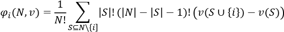
If necessary, you can consult the explanation of the expression in Chapter 4, Microsoft Azure Machine Learning Model Interpretability with SHAP. However, to help a user understand how we calculate marginal contributions, we are going to pull most of the expression out, which leaves us with the following:

This simplified expression can be explained as follows:
 is the marginal contribution of a word, i, that will be named
 mcc(marginal cognitive contribution) in the Python program of the next section.- S is the entire dataset. The limit of this experiment is that not all of the possible permutations are calculated.
 is the marginal cognitive contribution of all of the words preceding i in
 pdictionary, but not including i. is the prediction performance over the dataset when i is included.
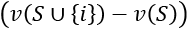 is the marginal value of i.
If we now express this in plain English, we obtain the following:
- The Python function will take the first word it finds in
pdictionary - It will consider that this is the only positive word to find in each review of the dataset
- Naturally, the number of true positives the function finds will be low because it's only looking for one word
- However, the performance of one word will be measured
- Then, the Python program adds the second word in
pdictionary, and the function obtains a better overall score - This new score is compared to the previous one and thereby provides the marginal contribution of the current word
We will not show this mathematical function to a user.
We will only show the Python program's outputs.
The Python marginal cognitive contribution function
The set of rules described in the previous section are applied in a marginal cognitive contribution function:
# @title Marginal cognitive contribution metrics
maxpl = pl
for mcc in range(0, pl):
  score = cognitive_xai(y, mcc, threshold)
  if mcc == 0:
    print(score, "The MCC is", score, "for", pdictionary[mcc])
    last_score = score
  if mcc > 0:
    print(score, "The MCC is",
          round(score - last_score, 4), "for", pdictionary[mcc])
    last_score = score
If we look at a random line of the output of the function, we see:
4 true positives 3489 scores 0.3515 0.6792 TP 9926 CTP 5137
0.3515 The MCC is 0.0172 for real
The first part of the output was displayed from the code of the main function described in the previous section:
def cognitive_xai(y, pl, threshold):
It can be interesting to go through the values again for maintenance reasons.
However, the key part to focus on is the sentence beginning with MCC.
In this example, the key phrase to observe is this one:
The MCC is 0.0172 for real
This means that when the word "real" was added to the list of words to find in a review, the accuracy of the system went up by a value of 0.0172.
All of the negative values are taken into account each time as a prerequisite.
With this in mind, observe the output of the whole marginal cognitive contribution process by reading the part of the output that states:
"The MCC is x for "word w"
You will see what each word adds to the performance of the model:
0 true positives 2484 scores 0.2503 0.667 TP 9926 CTP 3724
0.2503 The MCC is 0.2503 for good
1 true positives 2484 scores 0.2503 0.667 TP 9926 CTP 3724
0.2503 The MCC is 0.0 for excellent
2 true positives 2953 scores 0.2975 0.6938 TP 9926 CTP 4256
0.2975 The MCC is 0.0472 for interesting
3 true positives 3318 scores 0.3343 0.6749 TP 9926 CTP 4916
0.3343 The MCC is 0.0368 for hilarious
4 true positives 3489 scores 0.3515 0.6792 TP 9926 CTP 5137
0.3515 The MCC is 0.0172 for real
5 true positives 4962 scores 0.4999 0.6725 TP 9926 CTP 7378
0.4999 The MCC is 0.1484 for great
6 true positives 5639 scores 0.5681 0.685 TP 9926 CTP 8232
0.5681 The MCC is 0.0682 for loved
7 true positives 5747 scores 0.579 0.6877 TP 9926 CTP 8357
0.579 The MCC is 0.0109 for like
8 true positives 6345 scores 0.6392 0.6737 TP 9926 CTP 9418
0.6392 The MCC is 0.0602 for best
9 true positives 6572 scores 0.6621 0.6778 TP 9926 CTP 9696
0.6621 The MCC is 0.0229 for cool
10 true positives 6579 scores 0.6628 0.6771 TP 9926 CTP 9716
0.6628 The MCC is 0.0007 for adore
11 true positives 6583 scores 0.6632 0.6772 TP 9926 CTP 9721
0.6632 The MCC is 0.0004 for impressive
.../...
26 true positives 6792 scores 0.6843 0.6765 TP 9926 CTP 10040
0.6843 The MCC is 0.0016 for talented
27 true positives 6792 scores 0.6843 0.6765 TP 9926 CTP 10040
0.6843 The MCC is 0.0 for brilliant
28 true positives 6819 scores 0.687 0.6772 TP 9926 CTP 10070
0.687 The MCC is 0.0027 for genius
29 true positives 6828 scores 0.6879 0.6772 TP 9926 CTP 10082
0.6879 The MCC is 0.0009 for bright
30 true positives 6832 scores 0.6883 0.6771 TP 9926 CTP 10090
0.6883 The MCC is 0.0004 for creative
31 true positives 6836 scores 0.6887 0.677 TP 9926 CTP 10097
0.6887 The MCC is 0.0004 for fantastic
32 true positives 6844 scores 0.6895 0.677 TP 9926 CTP 10109
0.6895 The MCC is 0.0008 for interesting
33 true positives 6844 scores 0.6895 0.677 TP 9926 CTP 10109
0.6895 The MCC is 0.0 for recommend
34 true positives 6883 scores 0.6934 0.6769 TP 9926 CTP 10169
0.6934 The MCC is 0.0039 for encourage
35 true positives 6885 scores 0.6936 0.6769 TP 9926 CTP 10171
0.6936 The MCC is 0.0002 for go
36 true positives 7058 scores 0.7111 0.6699 TP 9926 CTP 10536
0.7111 The MCC is 0.0175 for admirable
37 true positives 7060 scores 0.7113 0.67 TP 9926 CTP 10538
0.7113 The MCC is 0.0002 for irrestible
38 true positives 7060 scores 0.7113 0.67 TP 9926 CTP 10538
0.7113 The MCC is 0.0 for special
39 true positives 7088 scores 0.7141 0.6696 TP 9926 CTP 10585
0.7141 The MCC is 0.0028 for unique
The performance of these words picked intuitively is enough to understand that the more words you observe, the better the result.
The next steps would be to generate all the possible permutations and improve the system by adding other words to the dictionaries. Also, we could develop an HTML or Java interface to display the results in another format on a user-friendly web page.
In this section, we selected key features with our human cognitive ability. Let's now see how to fine-tune vectorizers that can approach our observation qualities.
A cognitive approach to vectorizers
AI and XAI outperform us in many cases. This is a good thing because that's what we designed them for! What would we do with slow and imprecise AI?
However, in some cases, we not only request an AI explanation, but we also need to understand it.
In Chapter 8, Local Interpretable Model-Agnostic Explanations (LIME), we reached several interesting conclusions. However, we left with an intriguing comment on the dataset.
In this section, we will use our human cognitive abilities, not only to explain, but to understand the third of the conclusions we made in Chapter 8:
- LIME can prove that even accurate predictions cannot be trusted without XAI
- Local interpretable models will measure to what extent we can trust a prediction
- Local explanations might show that the dataset cannot be trusted to produce reliable predictions
- Explainable AI can prove that a model cannot be trusted or that it is reliable
- LIME's visual explanations can be an excellent way to help a user trust an AI system
Note that in conclusion 3, the wording is might show. We must be careful because of the number of parameters involved in such a model.
Let's see why by exploring the vectorizer.
Explaining the vectorizer for LIME
Open LIME.ipynb, which is the program we explored in Chapter 8, Local Interpretable Model-Agnostic Explanations (LIME). We are going to go back to the vectorizer in that code.
In Chapter 8, we wanted to find the newsgroup a discussion belonged to.
As humans, we know that in the English language, we will find a very long set of words that can belong in any newsgroup, such as:
set A = words found in any newsgroup = {in, out, over, under, to, the, a, these, those, that, what, where, how, ..., which}
As humans, we also know that these words are more likely to appear than words bearing a meaning or that relate to a specific area, such as:
set B = words not found in any newsgroup = {satellites, rockets, make-up, cream, fish, ..., meat}.
As humans, we then conclude that the words of set A will have a higher frequency value in a text than the words of set B.
Scikit-learn's vectorizer has an option that will fit our human conclusion: min_df.
min_df will vectorize words with a frequency exceeding the minimum frequency specified. We will now go back to the vectorizer in the program and we can add the min_df parameter:
vectorizer = sklearn.feature_extraction.text.TfidfVectorizer(
    min_df=20, lowercase=False)
You can experiment with several min_df values to see how the LIME explainer reacts.
min_df will detect the words that appear more than 20 times and prune the vectors. The program will drop many words that blurred LIME's explainer, such as "in," "our," "out," and "up."
We can also comment the LIME feature dropping function and let the explainer examine a wider horizon since we have reduced the volume of features taken into account:
"""
# @title Removing some features
print('Original prediction:',
      rf.predict_proba(test_vectors[idx])[0, 1])
tmp = test_vectors[idx].copy()
tmp[0, vectorizer.vocabulary_['Posting']] = 0
tmp[0, vectorizer.vocabulary_['Host']] = 0
print('Prediction removing some features:',
      rf.predict_proba(tmp)[0, 1])
print('Difference:', rf.predict_proba(tmp)[0, 1] –
                     rf.predict_proba(test_vectors[idx])[0, 1])
"""
If we run the program again and look at LIME's summary, the text of index 5 (random sampling may change this example), we obtain a better result:

Figure 12.2: A LIME explainer plot
We can see that the prediction of 0.79 for electronics seems better, and the explanation has actually improved! Three features stand out for electronics:
electronics = {"capacitor", "resistors", "resistances"}
Note that the example might change from one run to another due to random sampling and the parameters you tweak.
We can now interpret one of the conclusions we made differently:
Local explanations might show that the dataset cannot be trusted to produce reliable predictions.
This conclusion can now be understood in light of our manual human cognitive brain's analysis:
Local explanations might show that the dataset contains features that fit both categories to distinguish. In that case, we must find the common features that blur the results and prune them with the vectorizer.
We can now make a genuine human conclusion:
Once a user has an explanation that doesn't meet expectations, the next step will be to involve a human to investigate and contribute to the improvement of the model. No conclusion can be made before investigating the causes of the explanations provided. No model can be improved if the explanations are not understood.
Let's apply the same method we applied to the vectorizer to a SHAP model.
Explaining the IMDb vectorizer for SHAP
In this section, we will use our knowledge of the vectorizer to see whether we can approach the human cognitive analysis of the IMDb dataset by pruning features.
In the Cognitive rule-based explanations section of this chapter, we created intuitive cognitive dictionaries from a human perspective.
Let's see how close the vectorizer's output and the human input can get to each other.
Open Cognitive_XAI_IMDB_12.ipynb again and go to the Vectorize datasets cell. We will add the min_df parameter, as we did in the previous section.
However, this time, we know that the dataset contains a massive amount of data. Intuitively, as in the previous section, we will prune the features accordingly.
This time, we set the minimum frequency value of a feature to min_df = 1000, as shown in the following code snippet:
# @title Vectorize datasets
# vectorizing
display = 1 # 0 no display, 1 display
vectorizer = TfidfVectorizer(min_df=1000, lowercase=False)
We now focus on fitting the training dataset:
X_train = vectorizer.fit_transform(corpus_train)
The program is now ready for our experiments.
We first retrieve the features' names and display some basic information:
# visualizing the vectorized features
feature_names = vectorizer.get_feature_names()
lf = (len(feature_names))
print("Number of features", lf)
if display == 1:
  for fv in range(0, lf):
    print(feature_names[fv], round(vectorizer.idf_[fv],5))
The output will produce the number of features and display them:
Number of features 434
Number of features 434
10 3.00068
After 3.85602
All 3.5751
American 3.74347
And 2.65868
As 3.1568
At 3.84909
But 2.55358
DVD 3.60509...
We did not need to limit the number of features to display since we pruned a large number of tokens (words). Only 434 features are left.
We will now add a function that will compare the human-made dictionary of The dictionaries section of this chapter with the feature names produced by the optimized vectorizer.
The program first looks for the positive contributions that are contained in both the human-made pdictionary and feature_names produced by the vectorizer:
# @title Cognitive min vectorizing control
lf = (len(feature_names))
if display == 1:
  print("Positive contributions:")
  for fv in range(0, lf):
    for check in range(0, pl):
      if (feature_names[fv] == pdictionary[check]):
        print(feature_names[fv], round(vectorizer.idf_[fv], 5),)
The program then looks for the negative contributions that are contained in both the human-made ndictionary and feature_names produced by the vectorizer:
  print("
")
  print("Negative contributions:")
  for fv in range(0, lf):
    for check in range(0, threshold):
      if(feature_names[fv] == ndictionary[check]):
        print(feature_names[fv], round(vectorizer.idf_[fv], 5))
Some of our human-made words are not present in the vectorizer, although they contribute to a prediction. However, the ones in common with the vectorizer have high values:
Positive contributions:
beautiful 3.66936
best 2.6907
excellent 3.71211
go 2.84016
good 1.98315
great 2.43092
interesting 3.27017
interesting 3.27017
like 1.79004
pretty 3.1853
real 2.94846
recommend 3.75755
special 3.69865
Negative contributions:
bad 2.4789
poor 3.82351
terrible 3.95368
worst 3.46163
In Chapter 4, Microsoft Azure Machine Learning Model Interpretability with SHAP, the SHAP module in SHAP_IMDB.ipynb explained a prediction.
In this section, we compared what humans would intuitively do with SHAP's mathematical explanation. We first executed the process with a rules-based approach in the Cognitive rule-based explanations section of this chapter.
We have shown how to help a user go from machine intelligence explanations to human cognitive understanding.
We will now see how our human cognitive power can speed up a CEM result.
Human cognitive input for the CEM
In this section, we will use our human cognitive abilities to pick two key features out of tens of features inside a minute and solve a problem.
In Chapter 9, The Counterfactual Explanations Method, we used WIT to visualize the counterfactuals of data points. The data points were images of people who were smiling or not smiling. The goal was to predict the category in which a person was situated.
We explored Counterfactual_explanations.ipynb. You can go back and go through this if necessary. We found that some pictures were confusing. For example, we examined the following images:

Figure 12.3: WIT interface displaying counterfactual data points
It is difficult to see whether the person on the left is smiling.
This leads us to find a cognitive explanation.
Rule-based perspectives
Rule bases can be effective when machine learning or deep learning models reach their explainable AI limits.
In this section, we will set out the ground for rule bases in datasets. Rule bases are based on cognitive approaches or other machine learning algorithms. In this case, we will create human-designed rules.
A productive approach, in our case, would be to control the AI system with a human-built rule base instead of letting the machine learning program run freely in its black box.
The advantage of this human-designed rule base is that it will alleviate the burden of mandatory human explanations once the program produces controversial outputs.
For example, take a moment to observe the column names of the CelebA dataset. Let's name the set of names C:
 C = {image_id, 5_o_Clock_Shadow, Arched_Eyebrows, Attractive,
      Bags_Under_Eyes, Bald, Bangs, Big_Lips, Big_Nose, Black_Hair,
      Blond_Hair, Blurry, Brown_Hair, Bushy_Eyebrows, Chubby,
      Double_Chin, Eyeglasses, Goatee, Gray_Hair, Heavy_Makeup,
      High_Cheekbones, Male, Mouth_Slightly_Open, Mustache,
      Narrow_Eyes, No_Beard, Oval_Face, Pale_Skin, Pointy_Nose,
      Receding_Hairline, Rosy_Cheeks, Sideburns, Smiling,
      Straight_Hair, Wavy_Hair, Wearing_Earrings, Wearing_Hat,
      Wearing_Lipstick, Wearing_Necklace, Wearing_Necktie, Young}
We can see that there are quite a number of features! We might want to give up and just let a machine learning or deep learning algorithm do the work. However, that is what this notebook did, and it's still not clear how the program produced its predictions.
We can apply a cognitive approach to prepare for the mandatory justifications we would have to provide if required.
Let's now examine how a human would eliminate features that cannot explain a smile. We would strike through the features that do not come into account.
This is a basic, everyday, common-sense cognitive approach we could apply to the dataset in a few minutes:
C = {image_id, 5_o_Clock_Shadow, Arched_Eyebrows, Attractive,
     Bags_Under_Eyes, Bald, Bangs, Big_Lips, Big_Nose, Black_Hair,
     Blond_Hair, Blurry, Brown_Hair, Bushy_Eyebrows, Chubby,
     Double_Chin, Eyeglasses, Goatee, Gray_Hair, Heavy_Makeup,
     High_Cheekbones, Male, Mouth_Slightly_Open, Mustache,
     Narrow_Eyes, No_Beard, Oval_Face, Pale_Skin, Pointy_Nose,
     Receding_Hairline, Rosy_Cheeks, Sideburns, Smiling,
     Straight_Hair, Wavy_Hair, Wearing_Earrings, Wearing_Hat,
     Wearing_Lipstick, Wearing_Necklace, Wearing_Necktie, Young}
A human would only take these features into account to see whether somebody is smiling. However, these three features are simply potential features until we go a bit further.
We will name the set of features a human would take into account to determine whether a person is smiling J. If we exclude irrelevant features, or features that are difficult to interpret, the column headers, we can retain:
![]() = the intersection between the column names C and J, the features a human would expect to see when a person is smiling.
= the intersection between the column names C and J, the features a human would expect to see when a person is smiling.
The result could be as follows:
 = {Mouth_Slightly_Open, Narrow_Eyes, Smiling}
We will exclude Smiling, which is a label of a class, not a real feature.
We will exclude Narrow_Eyes, which many humans have.
We are left with the following:
= {Mouth_Slightly_Open}
First, run the program we used in Chapter 9, The Counterfactual Explanations Method: Counterfactual_explanations.ipynb.
Now, we verify the conclusion we reached in WIT:
- Select Mouth_Slightly_Open in the Binning | X-Axis dropdown list:

Figure 12.4: Selecting a feature
- Select Inference score in the Color By dropdown list:

Figure 12.5: Selecting the inference score
- Select Inference value in the Label By dropdown list:

Figure 12.6: Selecting a label name
The binning divides the data points into two bins. The one on the left shows data points that do not contain our target feature.
The one on the right contains our target feature:

Figure 12.7: Visualizing a feature in bins
We can see that the bin on the right contains a significant amount of positive predictions (smiling people). The bin on the left only contains a sparse amount of positive predictions (smiling people).
In the bin on the left, the negative predictions (people who are not smiling) are dense and sparse in the bin on the right.
A justification rule that would filter the prediction of the AI system could be the following:
p is true if Mouth_Slightly_Open is true
However, many smiles are made with a closed mouth, such as the following true positive (the person is smiling):

Figure 12.8: Smiling without an open mouth
This means that Mouth_Slightly_Open is not the only rule a rule base would require. The second rule could be:
If lip corners are higher than the middle of the lips, the person could be smiling
This rule requires other rules as well.
The conclusions we can draw from this experiment are as follows:
- We took that program as it was, unconditionally
- The program was designed to make us think using WIT!
- We analyzed the data points
- We found that many features did not apply to an AI program that was detecting smiles
- We found that features were missing to predict whether a person was smiling
- In Chapter 9, The Counterfactual Explanations Method, we used the CEM to explain the distances between the data points
- In this chapter, we used everyday, common human cognitive sense to understand the problem
- This is an example of how explainable AI and cognitive human input can work together to help a user understand an explanation
In this section, we used human reasoning to go from explaining a machine learning output to understanding how the AI system arrived at a prediction.
Summary
In this chapter, we captured the essence of XAI tools and used their concepts for cognitive XAI. Ethical and moral perspectives lead us to create a cognitive explanation method in everyday language to satisfy users who request human intervention to understand AI-made decisions.
SHAP shows the marginal contribution of features. Facets displays data points in an XAI interface. We can interact with Google's WIT, which provides counterfactual explanations, among other functions.
The CEM tool shows us the importance of the absence of a feature as well as the marginal presence of a feature. LIME takes us right to a specific prediction and interprets the vicinity of a prediction. Anchors go a step further and explain the connections between the key features of a prediction.
In this chapter, we used the concepts of these tools to help a user understand the explanations and interpretations of an XAI tool. Cognitive AI does not have the model-agnostic quality of the XAI tools we explored. Cognitive AI requires careful human design. However, cognitive AI can provide human explanations.
We showed how cognitive AI could help a user understand sentiment analysis, marginal feature contributions, vectorizers, and how to grasp counterfactual models among the many other concepts of our XAI tools.
The XAI tools described in this chapter and book will lead to other XAI tools.
XAI will bridge the gap between the complexity of machine intelligence and the even more complex human understanding of the world.
The need for human intervention to explain AI will explode unless explainable and interpretable AI spreads. That's why XAI will spread to every area of AI.
In Chapter 7, A Python Client for Explainable AI Chatbots, we built the beginning of a human-machine relationship that will expand as the first level of XAI in a human-machine relationship. This relationship will involve AI, XAI, and connected smart objects and bots.
The human user will obtain personal assistant AI explanations at every moment to use the incredible technology that awaits us.
You will write the next chapter in your everyday life as a user, developer, or manager of AI and XAI!
Questions
- SHapley Additive exPlanations (SHAP) compute the marginal contribution of each feature with a SHAP value. (True|False)
- Google's What-If Tool can display SHAP values as counterfactual data points. (True|False)
- Counterfactual explanations include showing the distance between two data points. (True|False)
- The contrastive explanations method (CEM) has an interesting way of interpreting the absence of a feature in a prediction. (True|False)
- Local Interpretable Model-agnostic Explanations (LIME) interpret the vicinity of a prediction. (True|False)
- Anchors show the connection between features that can occur in positive and negative predictions. (True|False)
- Tools such as Google Location History can provide additional information to explain the output of a machine learning model. (True|False)
- Cognitive XAI captures the essence of XAI tools to help a user understand XAI in everyday language. (True|False)
- XAI is mandatory in many countries. (True|False)
- The future of AI is people-centered XAI that uses chatbots, among other tools. (True|False)
Further reading
For more on cognitive and human-machine (XAI) approaches, visit the following URL:
https://researcher.watson.ibm.com/researcher/view_group.php?id=7806