8

Local Interpretable Model-Agnostic Explanations (LIME)

The expansion of artificial intelligence (AI) relies on trust. Users will reject machine learning (ML) systems they cannot trust. We will not trust decisions made by models that do not provide clear explanations. An AI system must provide clear explanations, or it will gradually become obsolete.

Local Interpretable Model-agnostic Explanations (LIME)'s approach aims at reducing the distance between AI and humans. LIME is people-oriented like SHAP and WIT. LIME focuses on two main areas: trusting a model and trusting a prediction. LIME provides a unique explainable AI (XAI) algorithm that interprets predictions locally.

I recommend a third area: trusting the datasets. A perfect model and accurate predictions based on a biased dataset will destroy the bond between humans and AI. We have detailed the issue of ethical data in several chapters in this book, such as in Chapter 6, AI Fairness with Google's What-If Tool (WIT). In this chapter, instead of explaining why a dataset needs to meet ethical standards, I chose neutral datasets with information on electronics and space to avoid culturally biased datasets.

In this chapter, we will first define LIME and its unique approach. Then we will get started with LIME on Google Colaboratory, retrieve the data we need, and vectorize the datasets.

We will then create five machine learning models to demonstrate LIME's model-agnostic algorithm, train the model, and measure the predictions produced.

We will run an experimental AutoML module to compare the scores of the five ML models. The experimental AutoML module will run the ML models and choose the best one for the dataset. It will then automatically use the best model to make predictions and explain them with LIME.

Finally, we will build the LIME explainer to interpret the predictions with text and plots. We will see how the LIME explainer applies local interpretability to a model's predictions.

This chapter covers the following topics:

• Introducing LIME
• Running LIME on Google Colaboratory
• Retrieving and vectorizing datasets
• An experimental AutoML module
• Creating classifiers with a model-agnostic approach
• Random forest
• Bagging
• Gradient boosting
• Decision trees
• Extra trees
• Prediction metrics
• Vectorizing pipelines
• Creating a LIME explainer
• Visualizing LIME's text explanations
• LIME XAI plots

Our first step will be to understand AI interpretability with LIME.

Introducing LIME

LIME stands for Local Interpretable Model-agnostic Explanations. LIME explanations can help a user trust an AI system. A machine learning model often trains at least 100 features to reach a prediction. Showing all these features in an interface makes it nearly impossible for a user to analyze the result visually.

In Chapter 4, Microsoft Azure Machine Learning Model Interpretability with SHAP, we used SHAP to calculate the marginal contribution of a feature to the model and for a given prediction. The Shapley value of a feature represents its contribution to one or several sets of features. LIME has a different approach.

LIME wants to find out whether a model is locally faithful regardless of the model. Local fidelity verifies how a model represents the features around a prediction. Local fidelity might not fit the model globally, but it explains how the prediction was made. In the same way, a global explanation of the model might not explain a local prediction.

For example, we helped a doctor conclude that a patient was infected by the West Nile virus in Chapter 1, Explaining Artificial Intelligence with Python.

Our global feature set was as follows:

features = {colored sputum, cough, fever, headache, days, france, chicago, class}

Our global assumption was that the following main features led to the conclusion with a high probability value that the patient was infected with the West Nile virus:

features = {bad cough, high fever, bad headache, many days, chicago=true}

Our predictions relied on that ground truth.

But was this global ground truth always verified locally? What if a prediction was true for the West Nile virus with a slightly different set of features—how could we explain that locally?

LIME will explore the local vicinity of a prediction to explain it and analyze its local fidelity.

For example, suppose a prediction was a true positive for the West Nile virus but not precisely for the same reasons as our global model. LIME will search the vicinity of the instance of the prediction to explain the decision the model made.

In this case, LIME could find a high probability of the following features:

Local explanation = {high fever, mild sputum, mild headache, chicago=true}

We know that a patient with a high fever with a headache that was in Chicago points to the West Nile virus. The presence of chills might provide an explanation as well, although the global model had a different view. Locally, the prediction is faithful, although globally, our model's output was positive when many days and bad cough were present, and mild sputum was absent.

The prediction is thus locally faithful to the model. It has inherited the global feature attributes that LIME will detect and explain locally.

In this example, LIME did not take the model into account. LIME used the global features involved in a prediction and the local instance of the prediction to explain the output. In that sense, LIME is a model-agnostic model explainer.

We now have an intuitive understanding of what LIMEs are. We can now formalize LIME mathematically.

A mathematical representation of LIME

In this section, we will translate our intuitive understanding of LIME into a mathematical expression of LIME.

The original, global representation of an instance x can be represented as follows:

However, an interpretable representation of an instance is a binary vector:

The interpretable representation determines the local presence or absence of a feature or several features.

Let's now consider the model-agnostic property of LIME. represents a machine learning model. represents a set of models containing among other models:

As such, LIME's algorithm will interpret any other model in the same manner.

The domain of being a binary vector, we can represent it as follows:

Now, we face a difficult problem! The complexity of might create difficulties in analyzing the vicinity of an instance. We must take this factor into account. We will note the complexity of an interpretation of a model as follows:

We encountered such a complexity program in Chapter 2, White Box XAI for AI Bias and Ethics, when interpreting decision trees. When we began to explain the structure of a decision tree, we found that "the default output of a default decision tree structure challenges a user's ability to understand the algorithm." In Chapter 2, we fine-tuned the decision tree's parameters to limit the complexity of the output to explain.

We thus need to measure the complexity of a model with . High model complexity can hinder AI explanations and interpretations of a probability function f(x). must be reasonably low enough for humans to be able to interpret a prediction.

f(x) defines the probability that x belongs to the binary vector we defined previously, as follows:

The model can thus also be defined as follows:

Now, we need to add an instance z to see how x fits in this instance. We must measure the locality around x. For example, consider the features (in bold) in the two following sentences:

• Sentence 1: We danced all night; it was like in the movie Saturday Night Fever, or that movie called Chicago with that murder scene that sent chills down my spine. I listened to music for days when I was a teenager.
• Sentence 2: Doctor, when I was in Chicago, I hardly noticed a mosquito bit me, then when I got back to France, I came down with a fever.

Sentence 2 leads to a West Nile virus diagnosis.

However, a model could predict that Sentence 1 is a true positive as well.

The same could be said of the following Sentence 3:

• Sentence 3: I just got back from Italy, have a bad fever, and difficulty breathing.

Sentence 3 leads to a COVID-19 diagnosis that could be a false positive or not. I will not elaborate while in isolation in France at the time this book is being written. It would not be ethical to make mathematical models for educational purposes in such difficult times for hundreds of millions of us around the world.

In any case, we can see the importance of a proximity measurement between an instance z and the locality around x. We will define this proximity measurement as follows:

We now have all the variables we need to define LIME, except one important one. How faithful is this prediction to the global ground truth of our model? Can we explain why it is trustworthy? The answer to our question will be to determine how unfaithful a model can be when calculating f in the locality .

For all we know, a prediction could be a false positive! Or the prediction could be a false negative! Or even worse, the prediction could be a true positive or negative for the wrong reasons. This shows how unfaithful can be.

We will measure unfaithfulness with the letter .

will measure how unfaithful is when making approximations of f in the locality we defined as .

We must minimize unfaithfulness with and find how to keep the complexity as low as possible.

Finally, we can define an explanation generated by LIME as follows:

LIME will draw samples weighted by to optimize the equation to produce the best interpretation and explanations regardless of the model implemented.

LIME can be applied to various models, fidelity functions, and complexity measures. However, LIME's approach will follow the method we have defined.

For more on LIME theory, consult the References section at the end of this chapter.

We can now get started with this intuitive view and mathematical representation of LIME in mind!

Getting started with LIME

In this section, we will install LIME using LIME.ipynb, a Jupyter Notebook on Google Colaboratory. We will then retrieve the 20 newsgroups dataset from sklearn.datasets.

We will read the dataset and vectorize it.

The process is a standard scikit-learn approach that you can save and use as a template for other projects in which you implement other scikit-learn models.

We have already used this process in Chapter 4, Microsoft Azure Machine Learning Model Interpretability with SHAP. In this chapter, we will not examine the dataset from an ethical perspective. I chose one with no ethical ambiguity.

We will directly install LIME, then import and vectorize the dataset.

Let's now start by installing LIME on Google Colaboratory.

Installing LIME on Google Colaboratory

Open LIME.ipynb. We will be using LIME.ipynb throughout this chapter. The first cell contains the installation command:

# @title Installing LIME
try:
  import lime
except:
  print("Installing LIME")
  !pip install lime

The try/except will try to import lime. If lime is not installed, the program will crash. In this code, except will trigger !pip install lime.

Google Colaboratory deletes some libraries and modules when you restart it, as well as the current variables of a notebook. We then need to reinstall some packages. This piece of code will make the process seamless.

We will now retrieve the datasets.

Retrieving the datasets and vectorizing the dataset

In this section, we will import the program's modules, import the dataset, and vectorize it.

We first import the main modules for the program:

# @title Importing modules
import lime
import sklearn
import numpy as np
from __future__ import print_function
import sklearn
import sklearn.ensemble
import sklearn.metrics
from sklearn.ensemble import BaggingClassifier
from sklearn.neighbors import KNeighborsClassifier
from sklearn.ensemble import GradientBoostingClassifier
from sklearn.tree import DecisionTreeClassifier
from sklearn.ensemble import ExtraTreesClassifier

sklearn is the primary source of the models used in this program. sklearn also provides several datasets for machine learning. We will import the 20 newsgroups dataset:

# @title Retrieving newsgroups data
from sklearn.datasets import fetch_20newsgroups

A quick investigation of the source of this dataset is good practice, although the newsgroup we will choose contains no obvious ethical issues. The 20 newsgroups dataset contains thousands of newsgroups documents widely used for machine learning purposes. Scikit-learn offers more real-world datasets that you can explore with this program at https://scikit-learn.org/stable/datasets/index.html#real-world-datasets.

We now import two newsgroups from the dataset and label them:

categories = ['sci.electronics', 'sci.space']
newsgroups_train = fetch_20newsgroups(subset='train',
                                      categories=categories)
newsgroups_test = fetch_20newsgroups(subset='test',
                                     categories=categories)
class_names = ['electronics', 'space']

The models in this notebook will classify the content of these newsgroups in two classes: 'electronics' and 'space'.

The program classifies the datasets using vectorized data.

The text is vectorized and transformed into token counts, as explained and displayed in Chapter 4, Microsoft Azure Machine Learning Model Interpretability with SHAP:

# @title Vectorizing
vectorizer = sklearn.feature_extraction.text.TfidfVectorizer(
    lowercase=False)
train_vectors = vectorizer.fit_transform(newsgroups_train.data)
test_vectors = vectorizer.transform(newsgroups_test.data)

The dataset has been imported and vectorized. We can now focus on an experimental AutoML module.

An experimental AutoML module

In this section, we will implement ML models in the spirit of LIME. We will play by the rules and try not to influence the outcome of the ML models, whether we like it or not.

Each model will be treated equally as part of , our set of models:

We will implement five machine learning models with their default parameters, as provided by scikit-learn's example code.

We will then run all five machine learning models in a row and select the best one with an agnostic scoring system to make predictions for the LIME explainer.

Each model will be created with the same template and scoring method.

This experimental model will only choose the best model. If you wish to add features to this experiment, you can run epochs. You can develop functions that will change the parameters of the module during each epoch to try to improve it.

For this experiment, we do not want to influence outputs by tweaking the parameters.

Let's create the template we will be using for all five models.

Creating an agnostic AutoML template

In this section, we will create five models using the following template I initially designed for a random forest classifier.

The AutoML experiment begins by creating two optimizing variables. It is a small AutoML experiment limited to the goal of this section.

best will contain the score of the best model at the end of the evaluation phase, as follows:

# @title AutoML experiment: Score measurement variables
best = 0 # best classifier score

clf will contain the name of the best model at the end of the evaluation phase, as follows:

clf = "None" # best classifier name

The score can vary from one run to another because of the randomized sampling methods involved.

The program creates each model, then trains and evaluates its performance using the following template:

# @title AutoML experiment: Random forest
rf1 = sklearn.ensemble.RandomForestClassifier(n_estimators=500)
rf1.fit(train_vectors, newsgroups_train.target)
pred = rf1.predict(test_vectors)

Before we continue, we need to describe how a random forest model makes predictions. In Chapter 2, White Box XAI for AI Bias and Ethics, we went through the theoretical definition of a decision tree. A random forest is an ensemble algorithm. An ensemble algorithm takes several machine learning algorithms to improve its performance. It usually produces better results than a single algorithm.

A random forest fits a number of decision trees, makes random subsamples of the dataset, and uses averaging to increase the performance of the model. In this model, n_estimators=500 represents a forest of 500 trees.

Each classifier of the five classifiers has its own name: {rf1, rf2, rf3, rf4, rf5}

Each trained classifier has its own metrics: {score1, score2, score3, score4, score5}

sklearn.metrics.f1_score evaluates each model's score, as follows:

score1 = sklearn.metrics.f1_score(newsgroups_test.target,
                                  pred, average='binary')

If the score of a model exceeds the best score of the preceding models, it becomes the best model:

if score1 > best:
  best = score1
  clf = "Random forest"
  print("Random forest has achieved the top score!", score1)
else:
  print("Score of random forest", score1)

If score1 > best, best will become the best score and clf the name of the best model. best memorizes score1, which is displayed as the top-ranking score.

If the model has achieved the best score, its performance is displayed as follows:

Random forest has achieved the top score! 0.7757731958762887

Each model will apply the same template.

We have implemented the random forest classifier. We will now create the bagging classifier.

Bagging classifiers

A bagging classifier is an ensemble meta-estimator that fits the model using random samples of the original dataset. In this model, the classifiers are based on the k-nearest neighbors classifier described in Chapter 1, Explaining Artificial Intelligence with Python:

# @title AutoML experiment: Bagging
rf2 = BaggingClassifier(KNeighborsClassifier(),
                        n_estimators=500, max_samples=0.5,
                        max_features=0.5)
rf2.fit(train_vectors, newsgroups_train.target)
pred = rf2.predict(test_vectors)
score2 = sklearn.metrics.f1_score(newsgroups_test.target,
                                  pred, average='binary')
if score2 > best:
  best = score2
  clf = "Bagging"
  print("Bagging has achieved the top score!", score2)
else:
  print("Score of bagging", score2)

Note a key parameter: n_estimators=500. If you do not set this parameter to 500, the default value is only 10 base estimators for the ensemble. If you leave it that way, the random forest classifier will end up as the best model, and bagging will produce a poor accuracy value.

However, if you set the number of base classifiers to 500, like for the random forest, then it will exceed the performance of the random forest classifier.

Also note that if you do not set the base classifier to KNeighborsClassifier(), the default classifier is a decision tree.

max_samples=0.5 represents the maximum proportion of samples that the classifier will draw to train each estimator.

max_features=0.5 represents the maximum number of features that an estimator will draw to train each sample.

The bagging model achieved a better score in this case than the random forest model with the same number of estimators:

Bagging has achieved the top score! 0.7942583732057416

Let's now add a gradient booster classifier to our experiment.

Gradient boosting classifiers

A gradient boosting classifier is an ensemble meta-estimator like the preceding models. It uses a differentiable loss function to optimize its estimators, generally decision trees.

n_estimators=500 will run 500 estimators to optimize its performance:

# @title AutoML experiment: Gradient boosting
rf3 = GradientBoostingClassifier(random_state=1, n_estimators=500)
rf3.fit(train_vectors, newsgroups_train.target)
pred = rf3.predict(test_vectors)
score3 = sklearn.metrics.f1_score(newsgroups_test.target,
                                  pred, average='binary')
if score3 > best:
  best = score3
  clf = "Gradient boosting"
  print("Gradient boosting has achieved the top score!", score3)
else:
  print("Score of gradient boosting", score3)

The performance of the gradient boosting model does not beat the preceding models:

Score of gradient boosting 0.7909319899244333

Let's add a decision tree to the experiment.

Decision tree classifiers

The decision tree classifier only uses one tree. It makes it difficult to beat the ensemble models.

In Chapter 2, White Box XAI for AI Bias and Ethics, we already went through the theoretical definition of a decision tree and its parameters.

In this project, the program creates the model with default models:

# @title AutoML experiment: Decision tree
rf4 = DecisionTreeClassifier(random_state=1)
rf4.fit(train_vectors, newsgroups_train.target)
pred = rf4.predict(test_vectors)
score4 = sklearn.metrics.f1_score(newsgroups_test.target,
                                  pred, average='binary')
if score4 > best:
  best = score4
  clf = "Decision tree"
  print("Decision tree has achieved the top score!", score4)
else:
  print("Score of decision tree", score4)

As expected, a single decision tree cannot beat ensemble estimators for this dataset:

Score of decision tree 0.7231352718078382

Finally, let's add an extra trees classifier.

Extra trees classifiers

The extra trees model appears as a good approach for this dataset. This meta-estimator fits a number of randomized decision trees using subsamples of the dataset and averaging methods to obtain the best performance possible.

As for the preceding meta-estimators, let's set n_estimators=500 so that each meta-estimator in our experiment generates the same number of estimators:

# @title AutoML experiment: Extra trees
rf5 = ExtraTreesClassifier(n_estimators=500, random_state=1)
rf5.fit(train_vectors, newsgroups_train.target)
pred = rf5.predict(test_vectors)
score5 = sklearn.metrics.f1_score(newsgroups_test.target,
                                  pred, average='binary')
if score5 > best:
  best = score5
  clf = "Extra trees"
  print("Extra trees has achieved the top score!", score5)
else:
  print("Score of extra trees", score5)

The extra trees model produces the best performance:

Extra Trees has achieved the Top Score! 0.818297331639136

We have now run the five models of our prototype of an AutoML experiment.

We will now use our program to interpret the scores.

Interpreting the scores

In this section, we will display the scores achieved by the five models. You can try to improve the performance of a model by fine-tuning the parameters.

You can also add several other models to measure their performance.

In this chapter, we will focus on the LIME model-agnostic explainer and let the program select the model that produces the best performance.

The program displays the AutoML experiment summary:

# @title AutoML experiment: Summary
print("The best model is", clf, "with a score of:", round(best, 5))
print("Scores:")
print("Random forest         :", round(score1, 5))
print("Bagging               :", round(score2, 5))
print("Gradient boosting     :", round(score3, 5))
print("Decision tree         :", round(score4, 5))
print("Extra trees           :", round(score5, 5))

The output displays the summary:

The best model is Extra Trees with a score of: 0.8183
Scores:
Random forest         : 0.77577
Bagging               : 0.79426
Gradient boosting     : 0.79093
Decision tree         : 0.72314
Extra trees           : 0.8183

The best model is stored in clf.

We have now found the best model for this dataset. We can start making and displaying predictions.

Training the model and making predictions

In this section, we will decide whether we will take the AutoML experiment's choice into account or not. Then we will run the final model chosen, train it, and finalize the prediction process.

The interactive choice of classifier

The notebook now displays a form where you can specify to activate the automatic process or not.

If you choose to set AutoML to On in the dropdown list, then the best model of the AutoML experiment will become the default model of the Notebook.

If not, choose Off in the AutoML dropdown list:

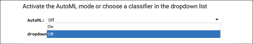
Figure 8.1: Activating AutoML or manually selecting a classifier

If you select Off, select the model you wish to choose for the LIME explainer in the dropdown list:

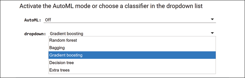
Figure 8.2: Selecting a classifier

Double-click on the form to view the code that manages the automatic process and the interactive selection:

# @title Activate the AutoML mode or
# choose a classifier in the dropdown list
AutoML = 'On' # @param ["On", "Off"]
dropdown = 'Gradient boosting' # @param ["Random forest",
                               #         "Bagging",
                               #         "Gradient boosting",
                               #         "Decision tree",
                               #         "Extra trees"]
if AutoML == "On":
  dropdown = clf
if clf == "None":
  dropdown = "Decision tree"
if dropdown == "Random forest":
  rf = sklearn.ensemble.RandomForestClassifier(n_estimators=500)
if dropdown == "Bagging":
  rf = BaggingClassifier(KNeighborsClassifier(), n_estimators=500,
                         max_samples=0.5, max_features=0.5)
if dropdown == "Gradient boosting":
  rf = GradientBoostingClassifier(random_state=1, n_estimators=500)
if dropdown == "Decision tree":
  rf = DecisionTreeClassifier(random_state=1)
if dropdown == "Extra trees":
  rf = ExtraTreesClassifier(random_state=1, n_estimators=500)

The AutoML experiment model or the model you chose will now train the data:

rf.fit(train_vectors, newsgroups_train.target)

We have reached the end of the AutoML experiment. We will continue by creating prediction metrics for the estimator.

Finalizing the prediction process

In this section, we will create prediction metrics and a pipeline with a vectorizer, and display the model's predictions.

The model chosen will be the AutoML experiment's choice if the automatic mode was turned on, or the model you select if the automatic mode was off.

First, we will start by creating the final prediction metrics for the selected model:

# @title Prediction metrics
pred = rf.predict(test_vectors)
sklearn.metrics.f1_score(newsgroups_test.target,
                         pred, average='binary')

The selected model's score will be displayed:

0.818297331639136

This score will vary every time you or the AutoML experiment changes models. It might also vary due to the random sampling processes during the training phase.

The program now creates a pipeline with a vectorizer to make predictions on the raw text:

# @title Creating a pipeline with a vectorizer
# Creating a pipeline to implement predictions on raw text lists
# (sklearn uses vectorized data)
from lime import lime_text
from sklearn.pipeline import make_pipeline
c = make_pipeline(vectorizer, rf)

Interception functions

We will now test the predictions. I added two records in the dataset to control the way LIME will explain them:

# @title Predictions
# YOUR INTERCEPTION FUNCTION HERE
newsgroups_test.data[1] = "Houston, we have a problem with our ice-cream out here in space. The ice-cream machine is out of order!"
newsgroups_test.data[2] = "Why doesn't my TV ever work? It keeps blinking at me as if I were the TV, and it was watching me with a webcam. Maybe AI is becoming autonomous!"

Note the following comment in the code:

# YOUR INTERCEPTION FUNCTION HERE

I will refer to them as the "interception records" in the The LIME explainer section.

You add an interception function here or at the beginning of the program to insert phrases you wish to test. To do this, you can consult the Intercepting the dataset section of Chapter 4, Microsoft Azure Machine Learning Model Interpretability with SHAP.

The program will print the text, which is in index 1 of the data object in this case. You can set it to another value to play with the model. However, in the next section, a form will make sure you do not choose an index that exceeds the length of the list. The prediction and text are displayed as follows:

print(newsgroups_test.data[1])
print(c.predict_proba([newsgroups_test.data[1]]))

The output shows the text and the prediction for both classes:

Houston, we have a problem with our ice-cream out here in space. The ice-cream machine is out of order!
[[0.266 0.734]]

We now have a trained model and have verified a prediction.

We can activate the LIME explainer to interpret the predictions.

The LIME explainer

In this section, we will implement the LIME explainer, generate an explanation, explore some simulations, and interpret the results with visualizations.

However, though I eluded ethical issues by selecting bland datasets, the predictions led to strange explanations!

Before creating the explainer in Python, we must sum up the tools we have before making interpretations and generating explanations.

We represented an equation of LIME in the A mathematical representation of LIME section of this chapter:

argmin searches the closest area possible around a prediction and finds the features that make a prediction fall into one class or another.

LIME will thus explain how a prediction was made, whatever the model is and however it reached that prediction.

Though LIME does not know which model was chosen by our experimental AutoML, we do. We know that we chose the best model, , among five models in a set named :

LIME does not know that we ran ensemble meta-estimators with 500 estimators and obtained reasonably good results in our summary:

The best model is Extra Trees with a score of: 0.8183
Scores:
Random Forest:        : 0.77577
Bagging               : 0.79426
Gradient Boosting     : 0.79093
Decision Tree         : 0.72314
Extra Trees           : 0.8183

We concluded that was the best model in G:

G = {"Random Forest", "Bagging", "Gradient Boosting", "Decision Trees", "Extra Trees"}

The extra trees classifier achieved a score of 0.81, which laid the ground for good and solid explanations.

We even created an interception function in the Interception functions section just like we did in Chapter 4, Microsoft Azure Machine Learning Model Interpretability with SHAP.

We should now expect the LIME explainer to highlight valuable features as we did in Chapter 4, Microsoft Azure Machine Learning Model Interpretability with SHAP, with our intercepted dataset.

But will we obtain the explanations we expected? We will see.

First, we need to create the LIME explainer and generate explanations.

Creating the LIME explainer

In this section, we will create the LIME explainer, select a text to explain, and generate an explanation.

The program first creates the explainer:

# @title Creating the LIME explainer
from lime.lime_text import LimeTextExplainer
explainer = LimeTextExplainer(class_names=class_names)

The explainer used the names of the classes defined when we imported the dataset:

class_names = ['electronics', 'space']

The program calculates the length of the dataset:

pn = len(newsgroups_test.data)
print("Length of newsgroup", pn)

In this case, the output is as follows:

Length of newsgroup 787

You can now select an index of the list in a form:

Figure 8.3: Selecting an index of the list

If you double-click on the form after choosing an index that exceeds the length of the dataset, the default value of the index will be 1:

# @title Selecting a text to explain
index = 5 # @param {type: "number"}
idx = index
if idx > pn:
  idx = 1
print(newsgroups_test.data[idx])

You can now see the content of this element of the list, as shown in this excerpt of a message:

From: [email protected] (C.M. Hicks)
Subject: Re: Making up odd resistor values required by filters
Nntp-Posting-Host: club.eng.cam.ac.uk
Organization: cam.eng
Lines: 26
[email protected] (Ian Hawkins) writes:
>When constructing active filters, odd values of resistor are often required
>(i.e. something like a 3.14 K Ohm resistor).(It seems best to choose common
>capacitor values and cope with the strange resistances then demanded).

The content of an index may change from one run to another due to the random sampling of the testing dataset.

Finally, the program generates an explanation for this message:

# @title Generating the explanation
exp = explainer.explain_instance(newsgroups_test.data[idx],
                                 c.predict_proba, num_features=10)
print('Document id: %d' % idx)
print('Probability(space) =',
      c.predict_proba([newsgroups_test.data[idx]])[0,1])
print('True class: %s' % class_names[newsgroups_test.target[idx]])

The output shows the document index, along with probability and classification information:

Document id: 5
Probability(space) = 0.45
True class: electronics

We created the explainer, selected a message, and generated an explanation.

We will now interpret the results produced by the LIME explainer.

Interpreting LIME explanations

In this section, we will interpret the results produced by the LIME explainer. I used the term "interpret" for a good reason.

To explain generally refers to making something clear and understandable. XAI can do that with the methods and algorithms we have implemented in this book.

In this section, we will see that explainable AI, AI explainability, or explaining AI are the best terms to describe a process by which a machine makes a prediction clear to a user.

To interpret implies more than just explaining. Interpreting means more than just looking at the context of a prediction and providing explanations. When we humans interpret something, we construe, we seek connections beyond the instance we are observing, beyond the context, and make connections that a machine cannot imagine.

To make things easier, in this book, I will continue to use "interpreting" AI loosely as a synonym for "explaining" AI.

However, bear in mind that it will take your human ability of interpretation and construal to understand the following sections.

Explaining the predictions as a list

The article in the Further reading section, "Why Should I Trust You?": Explaining the Predictions of Any Classifier, concludes that if something does not fit what we expected when we chose to use some newsgroups, the authors find that the model's predictions cannot be trusted.

In this section, we will try to understand why.

The program displays LIME's explanation as a list:

# @title Explain as a list
exp.as_list()

The output of the explanation of index 5 that we selected is no less than stunning!

Take a close look at the list of words that LIME highlighted and that influenced the prediction:

[('given', 0.07591981678565418),
 ('space', 0.05907439931403264),
 ('program', 0.031052797629092826),
 ('values', -0.01962286424974262),
 ('want', -0.019085470026052057),
 ('took', 0.018065064825319777),
 ('such', 0.017583164138156998),
 ('resistor', -0.015927676300306223),
 ('reported', 0.011573402045350527),
 ('was', 0.0076483181262587616)]

Each word has a negative or positive impact on the prediction. But this means nothing, as we will see now.

If we drop the "space" class name, we will get the following set W of LIME's explanations:

W = {"given", "program", "value", "want", "took", "resistor", "reported", "was"}

"resistor" could apply to a spacecraft or a radio.

If we try one of our interception function sentences, we obtain an overfitted explanation. Go back, choose 1 in the Selecting a text to explain form, and then rerun the program.

We first read the sentence:

Houston, we have a problem with our ice-cream out here in space. The ice-cream machine is out of order!

Then we look at LIME's explanation:

[('space', 0.2234448477494966),
 ('we', 0.05818967308950206),
 ('in', 0.015367276432916372),
 ('ice', -0.015137670461620763),
 ('of', 0.014242945006601808),
 ('our', 0.012470992672708379),
 ('with', -0.010137856356371086),
 ('Houston', 0.009826506741944144),
 ('The', 0.00836296328281397),
 ('machine', -0.0033670468609339615)]

We drop the "space" class name and create a set W' containing LIME's explanation. We will order the explanation as closely as possible to the original sentence:

W' = {"Houston", "we", "with", "our", "in", "the", "ice", "machine", "of"}

This explanation makes no sense either. Key features are not targeted.

If you try several index numbers randomly, you will find pertinent explanations from time to time.

However, at this point, we trust anything we see, so let's visualize LIME's explanations with a plot.

Explaining with a plot

In this section, we will visualize the explanations of the text in index 5 again. We will find nothing new. However, we will have a much better view of LIME's explanation.

First, LIME removes some of the features to measure the effect on the predictions:

# @title Removing some features
print('Original prediction:',
      rf.predict_proba(test_vectors[idx])[0, 1])
tmp = test_vectors[idx].copy()
tmp[0, vectorizer.vocabulary_['Posting']] = 0
tmp[0, vectorizer.vocabulary_['Host']] = 0
print('Prediction removing some features:',
      rf.predict_proba(tmp)[0, 1])
print('Difference:', rf.predict_proba(tmp)[0, 1] -
                     rf.predict_proba(test_vectors[idx])[0, 1])

This function will help a user simulate various local scenarios.

The output, in this case, does not change the prediction:

Original prediction: 0.334
Prediction removing some features: 0.336
Difference: 0.0020000000000000018

We now create the plot:

# @title Explaining with a plot
fig = exp.as_pyplot_figure()

The plot displays what we already know, but in a visually clear form:

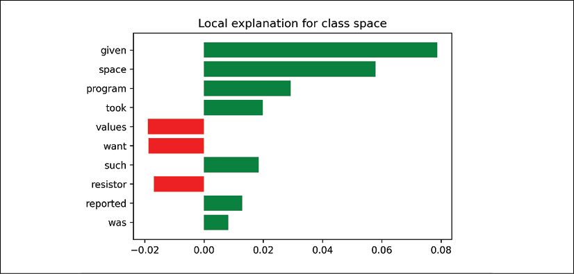
Figure 8.4: A local explanation for a prediction

We can see that words that relate to the positive impact on the class name space make no sense, such as: "given", "took", "such", "was", and "reported".

On the negative side, things aren't better with "want", for example.

This plot confirms the conclusions we will reach after the last verification.

We will now visualize the summary of the explanation in our notebook:

# @title Visual explanations
exp.show_in_notebook(text=False)

Let's save the explanations and display them in the HTML output:

# @title Saving explanation
exp.save_to_file('/content/oi.html')
# @title Showing in notebook
exp.show_in_notebook(text=True)

The visual HTML output contains the visual LIME explanations.

On the left, we can visualize the prediction probabilities:

Figure 8.5: The probabilities of a prediction

In the center, we can see the text explanations in a clear visual format:

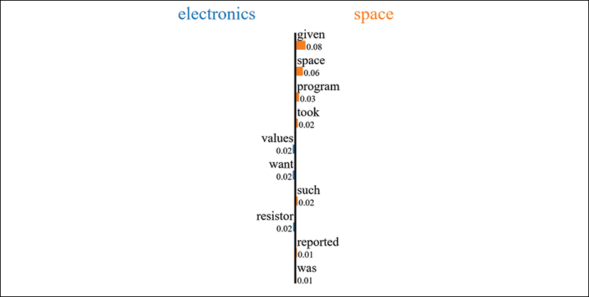
Figure 8.6: An explanation of the prediction

On the right side of the HTML output, we can consult the original text of this prediction and LIME explanation, as shown in this excerpt:

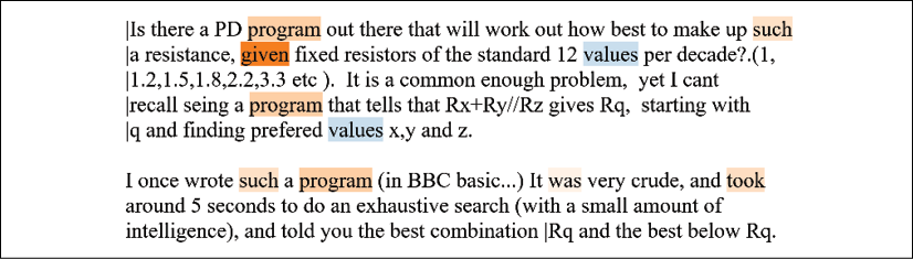
Figure 8.7: The original text of the prediction

LIME's explanation is shown in the text by highlighting the words used for the explanations. Each color (see color image) reflects the values calculated by LIME.

Conclusions of the LIME explanation process

We can draw several conclusions from the LIME process we implemented:

• LIME proves that even accurate predictions cannot be trusted without XAI
• Local interpretable models will measure to what extent we can trust a prediction
• Local explanations might show that the dataset cannot be trusted to produce reliable predictions
• XAI can prove that a model cannot be trusted or that it is reliable
• LIME's visual explanations can be an excellent way to help a user gain trust in an AI system

Note that in the third conclusion, the wording is might show. We must be careful because of the number of parameters involved in such a model. For example, in Chapter 12, Cognitive XAI, we will implement other approaches and investigate this third conclusion.

We can make only one global conclusion:

Once a user has an explanation that doesn't meet expectations, the next step will be to investigate and contribute to the improvement of the model. No conclusion can be made before investigating the causes of the explanations provided.

In this section, we proved that XAI is a prerequisite for any AI project, not just an option.

Summary

In this chapter, we confirmed that an AI system must base its approach on trust. A user must understand predictions and on what criteria an ML model produces its outputs.

LIME tackles AI explainability locally, where misunderstandings hurt the human-machine relationship. LIME's explainer does not satisfy itself with an accurate global model. It digs down to explain a prediction locally.

In this chapter, we installed LIME and retrieved newsgroup texts on electronics and space. We vectorized the data and created several models.

Once we implemented several models and the LIME explainer, we ran an experimental AutoML module. The models were all activated to generate predictions. The accuracy of each model was recorded and compared to its competitors. The best model then made predictions for LIME explanations.

Also, the final score of each model showed which model had the best performance with this dataset. We saw how LIME could explain the predictions of an accurate or inaccurate model.

The successful implementation of random forests, bagging, gradient boosting, decision trees, and extra trees models demonstrated LIME's model-agnostic approach.

Explaining and interpreting AI requires visual representations. LIME's plots transform the complexity of machine learning algorithms into clear visual explanations.

LIME shows once again that AI explainability relies on three factors: the quality of a dataset, the implementation of a model, and the quality of a model's predictions.

In the next chapter, The Counterfactual Explanation Method, we will discover how to explain a result with an unconditional method.

Questions

1. LIME stands for Local Interpretable Model-agnostic Explanations. (True|False)
2. LIME measures the overall accuracy score of a model. (True|False)
3. LIME's primary goal is to verify if a local prediction is faithful to the model. (True|False)
4. The LIME explainer shows why a local prediction is trustworthy or not. (True|False)
5. If you run a random forest model with LIME, you cannot use the same model with an extra trees model. (True|False)
6. There is a LIME explainer for each model. (True|False)
7. Prediction metrics are not necessary if a user is satisfied with predictions. (True|False)
8. A model that has a low accuracy score can produce accurate outputs. (True|False)
9. A model that has a high accuracy score provides correct outputs. (True|False)
10. Benchmarking models can help choose a model or fine-tune it. (True|False)

References

The reference code for LIME can be found at the following link:

https://github.com/marcotcr/lime

Further reading

• For more on LIME, see the following:
  • https://homes.cs.washington.edu/~marcotcr/blog/lime/
  • "Why Should I Trust You?": Explaining the Predictions of Any Classifier, https://arxiv.org/pdf/1602.04938v1.pdf
• For more on scikit-learn, see https://scikit-learn.org