4

Microsoft Azure Machine Learning Model Interpretability with SHAP

Sentiment analysis will become one of the key services AI will provide. Social media, as we know it today, forms a seed, not the full-blown social model. Our opinions, consumer habits, browsing data, and location history constitute a formidable source of data of AI models.

The sum of all of the information about our daily activities is challenging to analyze. In this chapter, we will focus on data we voluntarily publish on cloud platforms: reviews.

We publish reviews everywhere. We write reviews about books, movies, equipment, smartphones, cars, and sports—everything that exists in our daily lives. In this chapter, we will analyze IMDb reviews of films. IMDb offers datasets of review information for commercial and non-commercial use.

As AI specialists, we need to start running AI models on the reviews as quickly as possible. After all, the data is available, so let's use it! Then, the harsh reality of prediction accuracy changes our pleasant endeavor into a nightmare. If the model is simple, its interpretability poses little to no problem. However, complex datasets such as the IMDb review dataset contain heterogeneous data that make it challenging to make accurate predictions.

If the model is complex, even when the accuracy seems correct, we cannot easily explain the predictions. We need a tool to detect the relationship between local specific features and a model's global output. We do not have the resources to write an explainable AI (XAI) tool for each model and project we implement. We need a model-agnostic algorithm to apply to any model to detect the contribution of each feature to a prediction.

In this chapter, we will focus on SHapley Additive exPlanations (SHAP), which is part of the Microsoft Azure Machine Learning model interpretability solution. In this chapter, we will use the word "interpret" or "explain" for explainable AI. Both terms mean that we are providing an explanation or an interpretation of a model.

SHAP can explain the output of any machine learning model. In this chapter, we will analyze and interpret the output of a linear model that's been applied to sentiment analysis with SHAP. We will use the algorithms and visualizations that come mainly from Su-In Lee's lab at the University of Washington and Microsoft Research.

We will start by understanding the mathematical foundations of Shapley values. We will then get started with SHAP in a Python Jupyter Notebook on Google Colaboratory.

The IMDb dataset contains vast amounts of information. We will write a data interception function to create a unit test that targets the behavior of the AI model using SHAP.

Finally, we will explain reviews from the IMDb dataset with SHAP algorithms and visualizations.

This chapter covers the following topics:

• Game theory basics
• Model-agnostic explainable AI
• Installing and running SHAP
• Importing and splitting sentiment analysis datasets
• Vectorizing the datasets
• Creating a dataset interception function to target small samples of data
• Linear models and logistic regression
• Interpreting sentiment analysis with SHAP
• Exploring SHAP explainable AI graphs

Our first step will be to understand SHAP from a mathematical point of view.

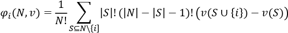
Introduction to SHAP

SHAP was derived from game theory. Lloyd Stowell Shapley gave his name to this game theory model in the 1950s. In game theory, each player decides to contribute to a coalition of players to produce a total value that will be superior to the sum of their individual values.

The Shapley value is the marginal contribution of a given player. The goal is to find and explain the marginal contribution of each participant in a coalition of players.

For example, each player in a football team often receives different amounts of bonuses based on each player's performance throughout a few games. The Shapley value provides a fair way to distribute a bonus to each player based on her/his contribution to the games.

In this section, we will first explore SHAP intuitively. Then, we will go through the mathematical explanation of the Shapley value. Finally, we will apply the mathematical model of the Shapley value to a sentiment analysis of movie reviews.

We will start with an intuitive explanation of the Shapley value.

Key SHAP principles

In this section, we will learn about Shapley values through the principles of symmetry, null players, and additivity. We will explore these concepts step by step with intuitive examples.

The first principle we will explore is symmetry.

Symmetry

If all of the players in a game have the same contribution, their contribution will be symmetrical. Suppose that, for a flight, the plane cannot take off without a pilot and a copilot. They both have the same contribution.

However, in a basketball team, if one player scores 25 points and another just a few points, the situation is asymmetrical. The Shapley value provides a way to find a fair distribution.

We will explore symmetry with an example. Let's start with equal contributions to a coalition.

a, b, c, and d are the four wheels of a car. Each wheel is necessary, which leads to the following consequences:

• v(N) = 1: v is the total value of a coalition. It is the total of the contribution of all four wheels. No sharing is possible. The car must have four wheels.

  N is the coalition, that is, the set, of wheels.

• S is a subset of N: In this case, S = 4. The value of the subset is the value of the coalition. The car cannot have less than four wheels.
• If , then v(S) = 0: If S, the subset of N, does not contain four wheels, then the value of S is 0 because the car is not complete. The contribution of this car S is 0.

Note that these four wheels are contributing independently to the coalition. Players in a basketball team, for example, contribute collectively to the coalition. However, game theory principles apply to both types of contributions.

Each wheel, a, b, c, and d, contributes equally to produce v(N) = 1. In this case, the contribution of each wheel is 1/4 = 0.25.

In this case, since v(a) = v(b), we can say that they are interchangeable. We can say that the values are symmetrical in cases such as this.

However, in many other cases, symmetry does not apply. We must find the marginal contribution of each member.

Before going further, we must explore the particular case of the null player.

Null player

A null player does not affect the outcome of a model. Suppose we now consider a player in a basketball team. During this game, the player was supposed to play offense. However, this player's leading partner, when playing offense, is suddenly absent. The player is both surprised and lost. For some reason, this null player will contribute nothing to the result of that specific game.

A null player's contribution to a coalition is null:

• is the Shapley value , the Greek letter phi, of this player, i.
• v is the total contribution of i in the coalition N, for example, a null player in a basketball team.
• N is the coalition of players.
• 0 represents the value of the contribution of the player, which is null in this case.

If we add i to a coalition, the coalition's global value will not increase since i's contribution is 0.

Fortunately, the Shapley values of a player can improve in other coalitions, which leads us to additivity.

Additivity

Our null basketball player, i, was lost in the previous game in the previous section. This player's performance added nothing to the overall performance of the team in game 1. The manager of the team realizes the talent of this player. Several players of the coalition are changed before the next game is played.

During the next two games, our null player, i, is in top shape; the player's leading partner is back. i scores over 20 points per game. The player is not a null player anymore. The contribution of this player has skyrocketed!

To be fair, the manager decides to measure the performance of our player in the past two games to determine her/his marginal contribution to the team, that is, the coalition:

• is the Shapley value of a player, i.
• is the Shapley value, the marginal contribution of a player over her/his last two games in different coalitions. Coaches constantly change the players in a team during and between games. We could extend the number of values to all of the coalitions the player encountered in a season to measure their additive marginal value.

The player's contribution is calculated over the addition of cooperative coalitions of the basketball season.

With that, we have explored some basic concepts of Shapley's value through symmetry, null players, and additivity.

We will now implement these concepts through a mathematical explanation of the Shapley value.

A mathematical expression of the Shapley value

In a coalition game (N, v), we need to find the payoff division. The payoff division is a unique fair distribution of the marginal contribution of each player to that player.

As such, the Shapley value will satisfy the null player, additivity, and symmetry/asymmetry properties we described in the previous sections.

In this section, we will begin to use words as players. Words are features in movie reviews, for example. Words are also players in game theory.

Words are sequence sensitive, which makes them an interesting way to illustrate Shapley values.

Consider the following three words in a set; that is, a coalition, N:

N = {excellent, not, bad}.

They seem deceivingly easy to understand and interpret in a review. However, if we begin to permute these three words, we will get several sequences, depending on the order they appear in. Each permutation represents a sequence of words that belong to S, a subset of three words that belong to N:

• S = {excellent, not bad}
• S₂ = {not excellent, bad}
• S₃ = {not bad, excellent}
• S₄ = {bad, not excellent}
• S₅ = {bad, excellent, not}
• S₆ = {excellent, bad, not}

We can draw several conclusions from these six subsets of N:

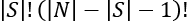
• The number of sequences or permutations of all of the elements of a set S is equal to S!. S! means multiply the chosen whole number from S down to 1. In this case, the number of elements in S = 3. The number of permutations of S is:

  S! = 3 × 2 × 1 = 6

  This explains why there are six sequences of the three words we are analyzing.

• In the first four subsets of S, the sequence of words completely changes the meaning of the phrase. This explains why we calculate the number of permutations.
• In the last two subsets, the meaning of the sequence is confusing, although they could be part of a longer phrase. For example, S₅ = {bad, excellent, not} could be part of a longer sequence such as {bad, excellent, not clear if I like this movie or not}.
• In this example, N contained three words, and we choose a subset S of N containing all three words. We could have selected a subset of S of N that only contained two words, such as S = {excellent, bad}.

We would now like to know the contribution of a specific word, i, to the meaning and sentiment (good or bad) of the phrase. This contribution is the Shapley value.

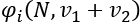
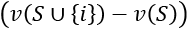
The Shapley value for a player i is expressed as follows:

Let's translate each part of this mathematical expression into natural language:

• is pronounced phi (the Shapley value) of i.

  means that the Shapley value phi of i in a coalition N with a value of v is equal to the terms that follow in the equation. At this point, we know that we are going to find the marginal contribution phi of i in a coalition N of value v. For example, we could like to know how much "excellent" contributed to the meaning of a phrase.

• means that the elements of S will be included in N but not i. We want to compare a set with and without i. If N = {excellent, not, bad}, S could be {bad, not} with i = excellent. If we compare S with and without "excellent," we will find a different marginal contribution value v.
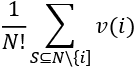
• will divide the sum (represented by the symbol ) of the value of all the possible values of i in all of the subsets S.
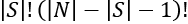• means that we are calculating a weight parameter to apply to the values. This weight multiplies all of the permutations of S! by the potential permutations of the remaining words that were not part of S. For example, if S = 2 because it contains {bad, not}, then N – S = 3 – 2 = 1. Then, we take i out represented by –1. You may be puzzled because this adds up to 0. However, keep in mind that 0! = 1.
• We now calculate the value v of a subset S of N containing i with the same subset with i:

  

  We now know the value of i for this permutation. For example, you can see the value of the word "excellent" in the following sentence that contains it, and the one after that doesn't:

  v(An excellent job) – v(a job) means that "excellent" has a high marginal value in this case.

Once every possible subset S of N has been evaluated, we will divide it evenly and fairly by N!, which represents the number of sequences of permutations we calculated:

We can now translate the Shapley value equation back into a mathematical expression:

We are now ready to calculate the Shapley value of a feature.

Sentiment analysis example

In this section, we will determine the Shapley value of two words, "good" and "excellent," in the following movie reviews. The format of each example is "[REVIEW TEXT]([MODEL PREDICTION OUTPUT])."

8 -1 r1 True I recommend that everybody go see this movie!
(5.33)
0 -1 r2 True This one is good and I recommend that everybody go see it!
(5.63)
2 12 r3 True This one is excellent and I recommend that everybody go see it!
(5.61)
4 26 r4 True This one is good and even excellent. I recommend that everybody go
(5.55)

The training and testing datasets are produced randomly. Each time you run the program, the records in the dataset might change, as well as the output values.

A positive prediction represents a positive sentiment. Words with high marginal contributions will increase the value of the model's output, regardless of the machine learning or deep learning model. This confirms that SHAP is model-agnostic.

Let's extract the information we are looking at and split the sentences into four categories from r1 to r3:

r1 good excluded and excellent excluded, 5.33
r2 good present and excellent excluded, 5.63
r3 excellent present and good excluded 5.61
r4 good present and excellent present 5.55

In this case, N = {good, excellent}.

We will apply the four categories to the following subsets of N:

• r1, , for which the prediction value of the model is v(S₁) = 5.33
• r2, S₂ = {good}, for which the prediction value of the model is v(S₂) = 5.63
• r3, S₃ = {excellent}, for which the prediction value of the model is v(S₃) = 5.61
• r4, S₄ = {good, excellent}, for which the prediction value of the model is v(S₄) = 5.61

The variables can now be plugged into the Shapley value equation:

r1 is represented by , for which the prediction value of the model is v(S₁) = 5.33. This will be the starting point of our analysis. We will use v(S₁) as the reference value of our calculations.

Shapley value for the first feature, "good"

What is the marginal contribution of the word "good" to the sentiment analysis of the reviews?

S₂ = {good}{good} = 0, meaning we are just comparing the marginal contribution of "good" to review r1, which contains neither "good" nor "excellent." The consequence of this is that there are only two possible subsets when i = good:

{good}, {good, excellent}

Thus, N! = 2 × 1 = 2 since there are only two sequences.

We will apply the variables to this part of the equation:

For i = " good," we now have:

S = 0, N = 2.

If we now plug all of the values in the permutations part of the equation, we obtain:

• S! = 0! = 1
• (N – S – 1) = 2 – 0 – 1 = 1
• S! (N – S – 1)! = 1 × 1 = 1, which we multiply the value v by

We will thus multiply the value of this permutation by 1:

We calculated the value of a set, r2, in which i ("good", in this case) is present and compared it to set r1, in which "good" is not present.

We obtained an intermediate value of 0.3.

This calculation is interesting. However, we would like to go further and find out how the words "good" and "excellent" cooperate in our coalition game. Which is the marginal value of the contribution of "excellent" in review r4 in which both words are present?

We will go back and apply the calculation method to the permutations part of the equation again:

• S = 1 because we are still calculating the value of "good" in set S₄ = {good, excellent} but S = {excellent}{good}
• (N – S – 1) = 2 – 1 – 1=0
• (N – S – 1)! = 0! = 1
• S! (N – S – 1)! = 1 × 1 = 1

Note that the contribution of "good" is negative in a sentence in which "excellent" is already present:

4 26 r4 True This one is good and even excellent. I recommend that everybody go
(5.55)

The redundant "good" and "excellent" do not add more meaning to this sentence. Let's finalize the Shapley value of "good."

We now have the values of the two sets when i = good:

• When S = {good} in r2, v = 0.3
• When S = {excellent} in r4, v = –0.8

Our last step is to plug the values into the beginning of the equation:

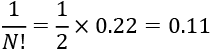
The sum of both permutations = 0.3 + (–0.8) = 0.22

We finally multiply this sum v(i) by the first part of the equation to obtain the marginal contribution of i = " good" for all permutations:

The Shapley value of "good" is:

We will now apply the same calculation to "excellent."

Shapley value for the second feature, "excellent"

We already know that the number of permutations is 1 for each feature we are calculating the Shapley value for. We are just replacing "good" with "excellent" in the same configuration:

We can now focus on the two possible permutations and their value.

First, we calculate the value of the permutation represented by r3, which only contains "excellent" and not "good," to r1, which contains neither "excellent" nor "good," to make a fair assumption:

Then, we calculate the value of the permutation represented by r3, which only contains "excellent," to r4, which contains both "excellent" and "good." The goal is to find the marginal contribution of "excellent":

Note that the contribution of "excellent" is negative in a sentence in which "good" is already present:

4 26 r4 True This one is good and even excellent. I recommend that everybody go
(5.55)

The redundant "good" and "excellent" do not add more meaning to this sentence. Let's finalize the Shapley value of "excellent."

The sum of both permutations = 0.28 + (–0.6) = 0.22

We finally multiply this sum v(i) by the first part of the equation to obtain the marginal contribution of i = good for all permutations:

The Shapley value of "excellent" is:

Verifying the Shapley values

We will now verify that the values we calculated.

The marginal contribution of "good" is equal to the marginal contribution of "excellent." Their combined contribution to a phrase that contains the sum of their respective values is thus:

If we examine the phrase that contains neither "good" nor "excellent," we will see that the value of the model's prediction is 5.33:

8 -1 r1 True I recommend that everybody go see this movie!
(5.33)

We also know the value of the model's prediction when both "good" and "excellent" are present:

4 26 r4 True This one is good and even excellent. I recommend that everybody go
(5.55)

We can verify that if i = "good" and j = "excellent" their total contribution, when added to the prediction of r1 (with neither "good" or "excellent"), will reach the value of the prediction p of r4 = 5.55:

We have verified our calculations.

Now that we know how to calculate a Shapley value, we can get started with a SHAP Python program.

Getting started with SHAP

In this section, we will first install SHAP. This version of SHAP includes algorithms and visualizations. The programs come mainly from Su-In Lee's lab at the University of Washington and Microsoft Research.

Once we have installed SHAP, we will import the data, split the datasets, and build a data interception function to target specific features.

Let's start by installing SHAP.

Open SHAP_IMDB.ipynb in Google Colaboratory. We will be using this notebook throughout this chapter.

Installing SHAP

You can install SHAP with one line of code:

# @title SHAP installation
!pip install shap

However, if you restart Colaboratory, you might lose this installation. You can verify if SHAP is installed with the following code:

# @title SHAP installation
try:
  import shap
except:
  !pip install shap

Next, we will import the modules we will be using.

Importing the modules

Each module has a specific prerequisite use in our project:

• import sklearn for the estimators and data processing functions.
• from sklearn.feature_extraction.text import TfidfVectorizer will transform the movie reviews, which are in text format into feature vectors, hence the term "vectorizer." The words become vocabulary tokens in a dictionary. The tokens then become feature indexes. The words of a review will then have their feature index counterparts. The converted reviews are then ready to become inputs for the estimator.

  TFIDF precedes vectorizer. The module extracts features from text and notes the term frequency (TF). The module also evaluates how important a word is through all the documents, which is named inverse document frequency (IDF).

• import numpy as np for its standard array and matrix functionality.
• import random will be used for random sampling of the datasets.
• import shap to implement the SHAP functions described in this notebook.

We are now all set to move, import, and split the data into training and testing datasets.

Importing the data

Our program must use SHAP to determine whether the review of a movie is positive or negative.

IMDb has made datasets available for commercial and non-commercial use with quite an amount of information: https://www.imdb.com/interfaces/.

The SHAP dataset we will import comes from https://github.com/slundberg/shap/blob/master/shap/datasets.py.

The code contains a function that retrieves IMDb sentiment analysis training data:

def imdb(display=False):
    """ Return the classic IMDB sentiment analysis training data in a nice package.
    Full data is at: http://ai.stanford.edu/~amaas/data/sentiment/aclImdb_v1.tar.gz
    Paper to cite when using the data is: http://www.aclweb.org/anthology/P11-1015
    """
    with open(cache(github_data_url + "imdb_train.txt")) as f:
        data = f.readlines()
    y = np.ones(25000, dtype=np.bool)
    y[:12500] = 0
    return data, y

As written in the code, the paper to cite when using the data is https://www.aclweb.org/anthology/P11-1015/.

We will now import the training set and its labels. In this section, we will import the original dataset. We will modify the data to track the impact of a specific feature in the Intercepting the dataset section of this chapter.

Let's start by importing the initial training dataset:

# @title Load IMDb data
corpus, y = shap.datasets.imdb()

We will start by intercepting the dataset to make sure we have examples we need for XAI.

Intercepting the dataset

Explainable AI requires clarity. The IMDb dataset contains only a limited amount of reviews. We want to make sure we can find samples that illustrate the explanation we described in the Sentiment analysis example section of this chapter.

We will intercept the dataset and insert samples that contain the key words we wish to analyze.

Unit tests

A unit test is designed to isolate a small example of what we wish to analyze. In corporate projects, we often carefully select the data to make sure the key concepts are represented. Our unit test will target specific keywords in the dataset.

In this chapter, for example, we would like to analyze the impact of the Shapley value of the word "excellent"(among other keywords) on the prediction of reviews of a specific movie. We would like to understand the reasoning of the SHAP algorithm at a detailed level.

Try to find the word "excellent" in the following random sample without using Ctrl + F:

Alan Johnson (Don Cheadle) is a successful dentist, who shares his practice with other business partners. Alan also has an loving wife (Jada Pinkett Smith) and he has two daughter (Camille LaChe Smith & Imani Hakim). He also let his parents stay in his huge apartment in New York City. But somehow, he feels that his life is somewhat empty. One ordinary day in the city, he sees his old college roommate Charlie Fireman (Adam Sandler). Which Alan hasn't seen Charlie in years. When Alan tries to befriends with Charlie again. Charlie is a lonely depressed man, who hides his true feelings from people who cares for him. Since Charlie unexpectedly loses his family in a plane crash, they were on one of the planes of September 11, 2001. When Alan nearly feels comfortable with Charlie. When Alan mentions things of his past, Charlie turns violent towards Alan or anyone who mentions his deceased family. Now Alan tries to help Charlie and tries to make his life a little easier for himself. But Alan finds out making Charlie talking about his true feelings is more difficult than expected.<br /><br />Written and Directed by Mike Bender (Blankman, Indian Summer, The Upside of Anger) made an wonderfully touching human drama that moments of sadness, truth and comedy as well. Sandler offers an impressive dramatic performance, which Sandler offers more in his dramatic role than he did on Paul Thomas Anderson's Punch-Drunk Love. Cheadle is excellent as usual. Pinkett Smith is fine as Alan's supportive wife, Liv Tyler is also good as the young psychiatrist and Saffron Burrows is quite good as the beautiful odd lonely woman, who has a wild crush on Alan. This film was sadly an box office disappointment, despite it had some great reviews. The cast are first-rate here, the writing & director is wonderful and Russ T. Alsobrook's terrific Widescreen Cinematography. The movie has great NYC locations, which the film makes New York a beautiful city to look at in the picture.<br /><br />DVD has an sharp anamorphic Widescreen (2.35:1) transfer and an good-Dolby Digital 5.1 Surround Sound. DVD also an jam session with Sandler & Cheadle, an featurette, photo montage and previews. I was expecting more for the DVD features like an audio commentary track by the director and deleted scenes. "Reign Over Me" is certainly one of the best films that came out this year. I am sure, this movie looked great in the big screen. Which sadly, i haven't had a chance to see it in a theater. But it is also the kind of movie that plays well on DVD. The film has an good soundtrack as well and it has plenty of familiar faces in supporting roles and bit-parts. Even the director has a bit-part as Byran Sugarman, who's an actor himself. "Reign Over Me" is one of the most underrated pictures of this year. It is also the best Sandler film in my taste since "The Wedding Singer". Don't miss it. HD Widescreen. (**** 1/2 out of *****).

If you did not find the word "excellent" by reading the text, use Ctrl + F to find it.

Now that you have found it, can you tell me what effect "excellent" has on the sentiment analysis of the review text of this movie?

That is where a unit test comes in handy. We want to make sure we will find samples that match the sentiment analysis scenario we wish to explain. We will now write a data interception function to create unit tests to make sure the dataset contains some basic explainable scenarios.

The data interception function

In this section, we will create a data interception function to implement our unit test keywords. Our unit test samples will contain the word "excellent" in one case and be omitted in other cases. We will thus be able to pinpoint the effect of a specific word in a SHAP analysis.

The interception function first starts with a trigger variable named interception:

# Interception
interception = 0 # 0 = IMDB raw data,
                 # 1 = data interception and simplification

If interception is set to 0, then the function will be deactivated, and the program will continue to use the original IMDb dataset. If interception is set to 1, then the function is activated:

# Interception
interception = 1 # 0 = IMDB raw data,
                 # 1 = data interception and simplification

A second parameter named display controls the interception function:

display = 2 # O = no, 1 = display samples, 2 = sample detection

display can be set to three values:

• display = 0: The display functions are deactivated
• display = 1: The first 10 samples of the training and testing data will be displayed
• display = 2: Specific samples are parsed to find explainable Shapley values

When the interception function is activated, the input data is intercepted.

In this case, four explainable reviews are created:

if interception == 1:
  good1 = "I recommend that everybody go see this movie!"
  good2 = "This one is good and I recommend that everybody go see it!"
  good3 = "This one is excellent and I recommend that everybody go see it!"
  good4 = "This one is good and even excellent. I recommend that everybody go see it!"
  bad = "I hate the plot since it's terrible with very bad language."

These four reviews will isolate reviews to explain Shapley values with SHAP graphs and with mathematics, as in the Sentiment analysis example section of this chapter.

We need to find the length of corpus before splitting it:

  x = len(corpus)
  print(x)

Our program will begin to intercept the original IMDb reviews and randomly replace them with the explainable Shapley value reviews we stored in five variables. The random variable is r with a value between 1 and 1000:

  for i in range(0, x):
    r = random.randint(1,2500)
    if y[i]:
      # corpus[i] = good1
      if (r <= 500): corpus[i] = good1;
      if (r > 500 and r <= 1000): corpus[i] = good2;
      if (r > 1000 and r <= 1700): corpus[i] = good3;
      if (r > 1700 and r <= 2500): corpus[i] = good4;
    if not y[i]:
      corpus[i] = bad

The function now displays the first 10 lines of the corpus. The data we inserted is our explainable data:

print("length", len(corpus)) # displaying samples of
                             # the training data
for i in range(0, 10):
  r = random.randint(1, len(corpus))
  print(r, y[r], corpus[r])

Note that we have transformed the corpus into a training set for our customized purposes, we will split the dataset into the actual training and testing subsets.

If display = 1, the first 10 reviews will be displayed:

if display == 1:
  print("y_test")
  for i in range(0, 20):
    print(i, y_test[i], corpus_test[i])
  print("y_train")
  for i in range(0, 1):
    print(i, y_train[i], corpus_train[i])

If display = 2, a rule base will isolate the cases we described in the Sentiment analysis example section of this chapter:

if display == 2:
  r1 = 0; r2 = 0; r3 = 0; r4 = 0; r5 = 0 # rules 1, 2, 3, 4, and 5
  y = len(corpus_test)
  for i in range(0, y):
    fstr = corpus_test[i]
    n0 = fstr.find("good")
    n1 = fstr.find("excellent")
    n2 = fstr.find("bad")
    if n0 < 0 and n1 < 0 and r1 == 0 and y_test[i]:
      r1 = 1 # without good and excellent
      print(i, "r1", y_test[i], corpus_test[i])
    if n0 >= 0 and n1 < 0 and r2 == 0 and y_test[i]:
      r2 = 1 # good without excellent
      print(i, "r2", y_test[i], corpus_test[i])
    if n1 >= 0 and n0 < 0 and r3 == 0 and y_test[i]:
      r3 = 1 # excellent without good
      print(i, "r3", y_test[i], corpus_test[i])
    if n0 >= 0 and n1 > 0 and r4 == 0 and y_test[i]:
      r4 = 1 # with good and excellent
      print(i, "r4", y_test[i], corpus_test[i])
    if n2 >= 0 and r5 == 0 and not y_test[i]:
      r5 = 1 # with bad
      print(i, "r5", y_test[i], corpus_test[i])
    if r1 + r2 + r3 + r4 + r5 == 5:
      break

The function will isolate the examples we inserted if it finds them or the samples that match the rules in the IMDb dataset.

We are now 100% sure that our unit test keywords are present. If necessary, we can explain SHAP with mathematics, a sentiment analysis example, and illustrate it with our unit keywords with our rule base.

Each rule counter is set to 0 at the beginning of the function:

if display == 2:
  r1 = 0; r2 = 0; r3 = 0; r4 = 0; r5 = 0 # rules 1, 2, 3, 4, and 5

The program determines the length of the testing dataset and then starts to parse the reviews:

  y = len(corpus_test)
  for i in range(0, y):

The function now stores a review in a string variable named fstr:

    fstr = corpus_test[i]
    n0 = fstr.find("good")
    n1 = fstr.find("excellent")
    n2 = fstr.find("bad")

The rule base is now applied:

    if n0 < 0 and n1 < 0 and r1 == 0 and y_test[i]:
      r1 = 1 # without good and excellent
      print(i, "r1", y_test[i], corpus_test[i])
    if n0 >= 0 and n1 < 0 and r2 == 0 and y_test[i]:
      r2 = 1 # good without excellent
      print(i, "r2", y_test[i], corpus_test[i])
    if n1 >= 0 and n0 < 0 and r3 == 0 and y_test[i]:
      r3 = 1 # excellent without good
      print(i, "r3", y_test[i], corpus_test[i])
    if n0 >= 0 and n1 > 0 and r4 == 0 and y_test[i]:
      r4 = 1 # with good and excellent
      print(i, "r4", y_test[i], corpus_test[i])
    if n2 >= 0 and r5 == 0 and not y_test[i]:
      r5 = 1 # with bad
      print(i, "r5", y_test[i], corpus_test[i])

Once all five rules are satisfied, the parsing function will stop:

    if r1 + r2 + r3 + r4 + r5 == 5:
      break

Five samples that fit the five rules are now displayed.

For example, an excerpt for r2 is:

0 r2 True "Twelve Monkeys" is odd and disturbing,...

The first column contains the review ID we will be able to track and use to explain SHAP values.

In this section, we intercepted the corpus to insert unit test reviews if the interception function is activated to make sure the dataset contains samples of the rules we set. If the interception function is not enabled, then the original dataset will be analyzed.

In both cases, our datasets are ready to be vectorized.

Vectorizing the datasets

In this section, we will vectorize the datasets with the TfidfVectorizer module we described in the Importing the data section of this chapter.

As a reminder, TfidfVectorizer extracts features from text and takes note of the term frequency (TF). The module also evaluates how important a word is. This process is named inverse document frequency (IDF).

The program first creates a vectorizer:

# @title Vectorize data
vectorizer = TfidfVectorizer(min_df=10)

min_df=10 will filter features—in our case, words—that have a document frequency lower than 10. Words that do not appear at least 10 times will be discarded.

We now vectorize the corpus_train and corpus_test datasets:

X_train = vectorizer.fit_transform(corpus_train)
X_test = vectorizer.transform(corpus_test)

What we can do now is visualize the frequency values that the vectorizer has attributed to the features of our dataset. It will be interesting to visualize the values we obtain to the feature values once a linear model has trained them to explain the evolution of the program. Then, we will visualize the Shapley values produced by SHAP.

Our first step is to visualize the frequency of the words we inserted using our interception function. This can be done on the IMDb dataset, but we recommend that you start with a small sample to understand the process.

Make sure interception=1 and then run the program up to the vectorizing cell. In this cell, we will add a display function to see the values that were calculated by the vectorizer, along with the feature names:

# visualizing the vectorized features
feature_names = vectorizer.get_feature_names()
lf = (len(feature_names))
for fv in range(0, lf):
  print(round(vectorizer.idf_[fv], 5), feature_names[fv])

The reviews that were created by the interception function have been transformed into a vectorized dictionary of words with their frequency values.

The output produces useful information:

1.92905 and
1.68573 bad
2.85347 even
1.70052 everybody
2.21593 excellent
1.70052 go
2.36576 good
1.68573 hate
1.92905 is
1.10691 it
1.68573 language
3.28824 movie
1.92905 one
1.68573 plot
1.70052 recommend
1.70052 see
1.68573 since
1.68573 terrible
1.70052 that
1.68573 the
1.70052 this
1.68573 very
1.68573 with

We can draw a couple of conclusions from the vectorized function we just ran:

• A small sample provides clear and useful information.
• We can see that the words "good," "excellent," and "bad" have higher values than most other words. "movie" has a positive contribution as well. This shows that the vectorizer has already identified the key features of our interception dataset.

The datasets have been vectorized, and we can already explain some of the feature values. We can now run the linear model.

Linear models and logistic regression

In this section, we will create a linear model, train it, and display the values of the features produced. We want to visualize the output of the linear model first. Then, we will explore the theoretical aspect of linear models.

Creating, training, and visualizing the output of a linear model

First, let's create, train, and visualize the output of a linear model using logistic regression:

# @title Linear model, logistic regression
model = sklearn.linear_model.LogisticRegression(C=0.1)
model.fit(X_train, y_train)

The program now displays the output of the trained linear model.

First, the program displays the positive values:

# print positive coefficients
lc = len(model.coef_[0])
for cf in range(0, lc):
  if (model.coef_[0][cf] >= 0):
    print(round(model.coef_[0][cf], 5), feature_names[cf])

Then, the program displays the negative values:

# print negative coefficients
for cf in range(0, lc):
  if (model.coef_[0][cf] < 0):
    print(round(model.coef_[0][cf], 5), feature_names[cf])

Before we analyze the output of the model, let's have a look at the reviews that were vectorized:

r1: good1="I recommend that everybody go see this movie!"
r2: good2="This one is good and I recommend that everybody go see it!"
r3: good3="This one is excellent and I recommend that everybody go see it!"
r4: good4="This one is good and even excellent. I recommend that everybody go see it!"
r5: bad="I hate the plot since it's terrible with very bad language."

With these reviews in mind, we can analyze how the linear model trained the features (words).

In natural language processing, we can also say that we are analyzing the "tokens" for the sequences of letters. In this chapter, we will continue to use the term "features" for "words."

The output of the program will first show the positive values and then the negative values:

1.28737 and
0.70628 even
1.71218 everybody
1.08344 excellent
1.71218 go
1.0073 good
1.28737 is
1.11644 movie
1.28737 one
1.71218 recommend
1.71218 see
1.71218 that
1.71218 this
-1.95518 bad
-1.95518 hate
-0.54483 it
-1.95518 language
-1.95518 plot
-1.95518 since
-1.95518 terrible
-1.95518 the
-1.95518 very
-1.95518 with

We can now see the impact of the linear model:

• The features (words) that are in the positive reviews have positive values
• The features (words) that are in the negative reviews have negative values

We can analyze a positive and negative review intuitively and classify them. In the following review, the key features (words) are obviously negative and will add up to a clearly negative review:

I hate(-1.9) the plot(-1.9) since it's terrible(-1.9) with very bad(-1.9) language.

In the following review, the key features (words) are obviously positive and will add up to a clearly positive review:

This one is good(1.0) and I recommend(1.7) that everybody(1.7) go see(1.7) it!

We can draw several conclusions from these examples:

• Although unit tests contain small samples, they represent an excellent way to explain models to users.
• Although unit tests contain small samples, they help clarify how models take inputs and produce outputs.
• A larger dataset will provide a variety of results, but it is better to start with a small sample. Analyzing large samples makes sense only once everybody in a team understands the model and has approved it.

We now have an intuitive understanding of a linear model. We will now explore the key theoretical aspects of linear models.

Defining a linear model

A linear model is a linear combination of weighted features that are used to reach a target. In our case, the linear model has been trained for a binary result—True or False for a positive review sample or a negative review sample, respectively.

A linear model can be expressed in the following equation, in which is the predicted value, is a feature, and is a weight or a coefficient in the following linear model equation:

A linear model requires methods to optimize regression to reach the defined target .

There are several regression methods available in the sklearn.linear_model module. We implemented the logistic regression method here.

Logistic regression fits our dataset well because the method is applied as a binary classification approach in our program, although it relies on regression. The probabilities are the outcomes modeled using a logistic function, which gives its name to the method.

The logistic function is a logistic sigmoid function and is one of the best ways to normalize the weights of an output. It can be defined as follows:

• e represents Euler's number, the natural logarithm, which is equal to 2.71828
• x is the value we wish to normalize

The logistic regression model can be displayed with:

print(model)

The output will show the values of parameters of the logistic regression model:

LogisticRegression(C=0.1, class_weight=None, dual=False,
                   fit_intercept=True, intercept_scaling=1,
                   l1_ratio=None, max_iter=100, multi_class='auto',
                   n_jobs=None, penalty='l2', random_state=None,
                   solver='lbfgs', tol=0.0001, verbose=0,
                   warm_start=False)

The program applied the following parameters to the logistic regression model. Once we understand the linear model function shown previously and we know that we are using a logistic regression function, we do not need to go into all of the details of the model's options unless we hit a rock. However, it is interesting to get an idea of the parameters the model takes into account. The program applied the following parameters to the logistic regression model:

• C=0.1 is a positive float that is the inverse of regularization strength. The smaller the value, the stronger the regularization.
• class_weight=None means that all the classes are supposed to have a class of one.
• dual=False is an optimization parameter used in conjunction with certain solvers.
• fit_intercept=True can be understood as a bias—an intercept—that will be added to the decision function if set to True.
• intercept_scaling=1 is a constant value that scales the inner calculation vectors of certain solvers.
• l1_ratio=None is used in conjunction with penalty when activated, which is not the case for our model.
• max_iter=100 represents the number of iterations it will take for the solvers to converge.
• multi_class='auto' in our case means that it will automatically choose the option that makes a binary problem fit for each label.
• n_jobs=None is the number of cores used when parallelizing over classes. In our case, None means only one core is used, which is enough for the datasets in this chapter.
• penalty='l2' is the norm for a penalty applied with 'lbfgs' solver, as used in this model.
• random_state=None in this case, this means that the seed of the random number generator will be generated by an instance using np.random.
• solver='lbfgs' is a solver that handles penalties such as 'l2'.
• tol=0.0001 is the stopping criteria expressed as a tolerance.
• verbose=0 activates verbosity if set to a positive number.
• warm_start=False means that the previous solution will be erased.

We have created and trained the model. Now, it is time to implement agnostic model explaining with SHAP.

Agnostic model explaining with SHAP

In the Introduction to SHAP section of this chapter, we saw that Shapley values rely on the input data and output data of a machine learning (ML) model. SHAP can interpret results. We went through the mathematical representation of the Shapley value without having to take a model into account.

Agnostic ML model explaining or interpreting will inevitably become a mandatory aspect of any AI project.

SHAP offers explainer models for several ML algorithms. In this chapter, we will focus on a linear model explainer.

Creating the linear model explainer

We will continue to add functions to SHAP_IMDB.ipynb.

Let's first create the linear explainer:

# @title Explain linear model
explainer = shap.LinearExplainer(model, X_train,
    feature_perturbation = "interventional")

Now, we will retrieve the Shapley values of the testing dataset:

shap_values = explainer.shap_values(X_test)

We must now convert the test dataset into an array for the plot function:

X_test_array = X_test.toarray() # we need to pass a dense version for
                                # the plotting functions

The linear explainer is ready. We can now create the plot function.

Creating the plot function

In this section, we will add a plot function to the program and explain a review to understand the process.

The plot function begins with a form where we can choose a review number from the dataset and then display a SHAP plot:

# @title Explaining reviews {display-mode: "form"}
review = 2 # @param {type: "number"}
shap.initjs()
ind = int(review)
shap.force_plot(explainer.expected_value, shap_values[ind,:],
                X_test_array[ind,:],
                feature_names=vectorizer.get_feature_names())

This program is a prototype. Make sure you enter small integers in the form since the test dataset's size varies each time the program is run:

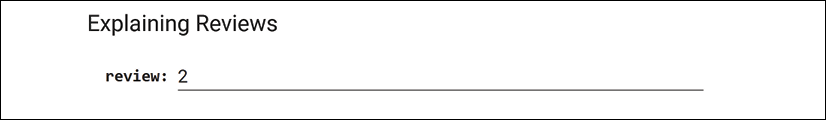
Figure 4.1: Enter small integers into the prototype

Once a review number is chosen, the model's prediction for that review will be displayed with the Shapley values that drove the prediction:

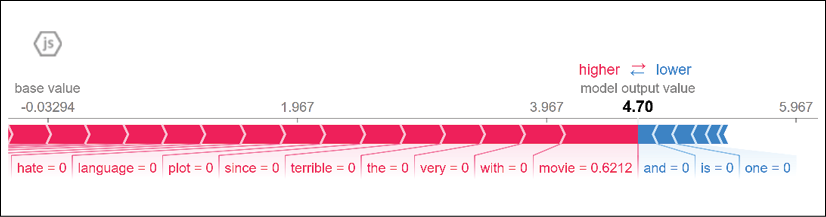
Figure 4.2: The Shapley values that determined the prediction

In this example, the prediction is positive. The sample review is:

I recommend that everybody go see this movie!

The Shapley values on the left (red in the color images) push the prediction to the right, to potentially positive results. In this example, the features (words) "recommend" and "see" contribute to a positive prediction:

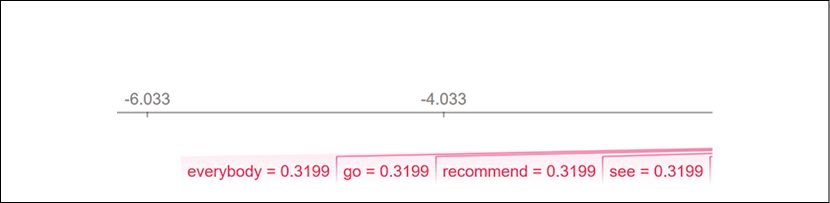
Figure 4.3: The Shapley values of words in a sequence

The Shapley values on the right (the blue color in the color images) push the prediction to the left, to potentially negative results.

The plot also shows a value name "base value," as you can see in Figure 4.4:

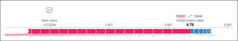
Figure 4.4: Visualizing the base value

Base value is the prediction the model would make if it did not take the features of the present dataset number output into account based on the whole dataset.

The SHAP plot we implemented explains and interprets the results with Shapley values. We can also retrieve interpretability information from the model's output.

Explaining the output of the model's prediction

SHAP's plot library explains the model's prediction visually. However, we can also add numerical explanations.

We will first check if the review is positive or negative and display it with its label:

# @title Review
print("Positive" if y_test[ind] else "Negative", "Review:")
print("y_test[ind]", ind, y_test[ind])

In this case, the label and review are:

True I recommend that everybody go see this movie!

The three features (words) we highlighted are worth investigating. We will retrieve the feature names and the corresponding Shapley values, and then display the result:

print(corpus_test[ind])
feature_names = vectorizer.get_feature_names()
lfn = len(feature_names)
lfn = 10 # choose the number of samples to display from [0, lfn]
for sfn in range(0, lfn):
  if shap_values[ind][sfn] >= 0:
    print(feature_names[sfn], round(X_test_array[ind][sfn], 5))
for sfn in range(0, lfn):
  if shap_values[ind][sfn] < 0:
    print(feature_names[sfn], round(X_test_array[ind][sfn], 5))

The output first displays the label of a review and the review:

Positive Review:
y_test[ind] 0 True
Positive Review:
y_test[ind] 2 True
I recommend that everybody go see this movie!

Note that lfn=10 limits the number of values displayed. The output will also vary, depending on the movie review number you choose.

The output then displays the features and their corresponding Shapley values:

bad 0.0
everybody 0.31982
go 0.31982
hate 0.0
it 0.0
language 0.0
movie 0.62151
plot 0.0
recommend 0.31982
see 0.31982

We can draw several conclusions from these explanations:

• The vectorizer generates the feature names for the whole dataset
• However, the Shapley values displayed in this section of the program are those of the review we are interpreting
• The Shapley values in this section of the code will differ from one review to another
• The highlighted features have marginal positive contribution Shapley values that explain the positive prediction
• The negative Shapley values are mostly equal to 0, which means that they will not influence the prediction

In this section, we created functions for visual and numerical SHAP explanations.

We will now explain the reviews from the intercepted dataset.

Explaining intercepted dataset reviews with SHAP

We have implemented the code and analyzed the Shapley value of a review. We will now analyze two more samples—one negative one and one positive one:

False I hate the plot since it's terrible with very bad language.
True This one is excellent and I recommend that everybody go see it!

Since the datasets are split into training and testing subsets randomly, the calculations will adapt to the new frequencies and the importance of a word.

We will first visualize the output of the negative review.

A negative review

The negative review contains three strong negative keywords and no positive features:

Negative Review:
y_test[ind] 1 False
I hate the plot since it's terrible with very bad language.

The negative features produce marginal negative contributions that push the prediction down to False, that is, a negative prediction for the review:

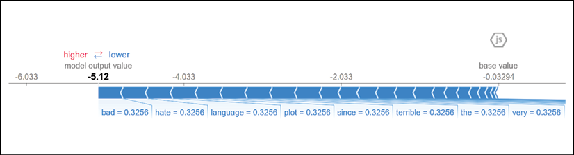
Figure 4.5: Showing the contribution of the words to Shapley values

We can observe that the feature "bad," for example, has a positive Shapley value in a negative review and that "excellent" does not contribute at all in this review:

Negative Review:
y_test[ind] 1 False
I hate the plot since it's terrible with very bad language.
and 0.0
bad 0.32565
even 0.0
everybody 0.0
excellent 0.0
go 0.0
good 0.0
hate 0.32565
is 0.0
it 0.21348
language 0.32565
movie 0.0
one 0.0
plot 0.32565
recommend 0.0
see 0.0
since 0.32565
terrible 0.32565
that 0.0
the 0.32565
this 0.0
very 0.32565
with 0.32565

Note the marginal contribution of the three key features of the review:

Key features = {bad, hate, terrible}

Now, observe how the marginal contributions of those key features change in a positive review.

A positive review

In a positive review, we now know that the key features will have Shapley values that prove their marginal contribution to the prediction:

This one is excellent and I recommend that everybody go see it!

First, observe that the marginal contribution of negative features has changed to null in this review:

Figure 4.6: Displaying the marginal contribution of negative features

However, the marginal contribution of the positive features has gone up:

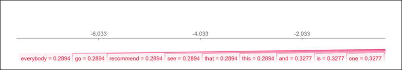
Figure 4.7: Displaying the marginal contribution of positive features

We can explain this analysis further by highlighting the negative features with no marginal contribution in this review:

Positive Review:
y_test[ind] 0 True
This one is excellent and I recommend that everybody go see it!
and 0.32749
bad 0.0
everybody 0.28932
excellent 0.37504
go 0.28932
hate 0.0
is 0.32749
language 0.0
one 0.32749
plot 0.0
recommend 0.28932
see 0.28932
since 0.0
terrible 0.0
that 0.28932
the 0.0
this 0.28932
very 0.0
with 0.0
even 0.0
good 0.0
it 0.18801
movie 0.0

The Shapley values of each feature change for each review, although they have a trained value for the whole dataset.

With that, we have interpreted a few samples from the intercepted datasets. We will now explain the reviews from the original IMDb dataset.

Explaining the original IMDb reviews with SHAP

In this section, we will interpret two IMDb reviews.

First, we must deactivate the interception function:

interception = 0

We have another problem to solve to interpret an IMDb review.

The number of words in the reviews of a movie exceeds the number of features we can detect visually. We thus need to limit the number of features the vectorizer will take into account.

We will go back to the vectorizer and set the value of min_df to 1000 instead of 100. We will have less features to explain how the program makes its predictions:

# vectorizing
vectorizer = TfidfVectorizer(min_df=1000)

In this case, we can still use the rules we hardcoded to find examples in the interception datasets. The probability of finding the keywords of the interception dataset such as "good," "excellent," and "bad" are very high.

You can change the values to find examples of features (words) you would like to analyze. You can replace "good," "excellent," and "bad" by your ideas to explore the outputs. You could target an actor, a director, a location, or any other information for which you would like to visualize the output of the model.

The code of our rule base remains without us making a single change:

  y = len(corpus_test)
  for i in range(0, y):
    fstr = corpus_test[i]
    n0 = fstr.find("good")
    n1 = fstr.find("excellent")
    n2 = fstr.find("bad")
    if n0 < 0 and n1 < 0 and r1 == 0 and y_test[i]:
      r1 = 1 # without good and excellent
      print(i, "r1", y_test[i], corpus_test[i])
    if n0 >= 0 and n1 < 0 and r2 == 0 and y_test[i]:
      r2 = 1 # good without excellent
      print(i, "r2", y_test[i], corpus_test[i])
    if n1 >= 0 and n0 < 0 and r3 == 0 and y_test[i]:
      r3 = 1 # excellent without good
      print(i, "r3", y_test[i], corpus_test[i])
    if n0 >= 0 and n1 > 0 and r4 == 0 and y_test[i]:
      r4 = 1 # with good and excellent
      print(i, "r4", y_test[i], corpus_test[i])
    if n2 >= 0 and r5 == 0 and not y_test[i]:
      r5 = 1 # with bad
      print(i, "r5", y_test[i], corpus_test[i])
    if r1 + r2 + r3 + r4 + r5 == 5:
      break

The program isolated five samples we can explain:

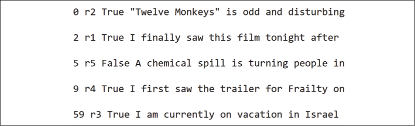
Figure 4.8: Five samples isolated by the program

We will start by analyzing a negative review.

A negative review sample

The text of the negative sample contains too many words to reproduce in this section. We can explain the prediction by analyzing a limited number of key features, such as the ones highlighted in the following excerpt:

{Bad acting, horribly awful special effects, and no budget to speak of}

These two features are driving the prediction down:

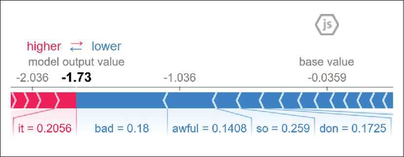
Figure 4.9: Analyzing the features that drove the prediction down

To confirm our interpretation, we can display the key features of the dataset and the Shapley values of the contribution of negative features to the Shapley values of the prediction:

although 0.0
always 0.0
american 0.0
an 0.06305
and 0.11407
anyone 0.0
as 0.0
awful 0.14078
back 0.0
bad 0.18
be 0.05787
beautiful 0.0
because 0.08745
become 0.0
before 0.0
beginning 0.0
best 0.0

We can apply the same key features sampling method to a positive review.

A positive review sample

Explainable AI tools require a method to isolate key aspects of the outputs of an ML algorithm. The goal is to break the dataset down into small data points so that we can interpret them visually.

We will now consider the following two excerpts of a positive review sample:

{but Young Adam and Young Fenton were excellent},
{really did a good job of directing it too.}

We will focus on the words "excellent" and "job" to interpret the output of the model:

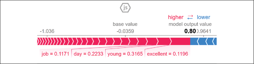
Figure 4.10: Visualizing the impact of "excellent"

Once again, we can prove that the Shapley values are correct for both excerpts:

ending 0.0
enough 0.0
entire 0.0
especially 0.11172
ever 0.0
every 0.0
excellent 0.11961
face 0.0
fact 0.0
fan 0.2442
far 0.0
felt 0.0
few 0.0
…/…
idea 0.0
if 0.0
instead 0.0
interesting 0.0
into 0.0
isn 0.0
it 0.14697
itself 0.0
job 0.11715
kids 0.0
kind 0.0
least 0.0
left 0.0
less 0.0
let 0.0

In this section, we created a linear logistic regression model and trained it. We then created a SHAP linear model explainer. Finally, we created SHAP visual explanation plots and numerical interpretation outputs.

Summary

In this chapter, we explored how to explain the output of a machine learning algorithm with an agnostic model approach using SHapley Additive exPlanations (SHAP). SHAP provides an excellent way to explain models by just analyzing their input data and output predictions.

We saw that SHAP relies on the Shapley value to explain the marginal contribution of a feature in a prediction. We started by understanding the mathematical foundations of the Shapley value. We then applied the Shapley value equation to a sentiment analysis example. With that in mind, we got started with SHAP.

We installed SHAP, imported the modules, imported the dataset, and split it into a training dataset and a testing dataset. Once that was done, we vectorized the data to run a linear model. We created the SHAP linear model explainer and visualized the marginal contribution of the features of the dataset in relation to the sentiment analysis predictions of reviews. A positive review prediction value would be pushed upward by high Shapley values for the positive features, for example.

To make explainable AI easier, we created unit tests of reviews using an interception function. Unit tests provide clear examples to explain an ML model rapidly.

Finally, once the interception function was built and tested, we ran SHAP on the original IMDb dataset to make further investigations on the marginal contribution of features regarding the sentiment analysis prediction of a review.

SHAP provides us with an excellent way to weigh the contribution of each feature with the Shapley values fair distribution equation. In the next chapter, Building an Explainable AI Solution from Scratch, we will build an XAI program using Facets and WIT.

Questions

1. Shapley values are model-dependent. (True|False)
2. Model-agnostic XAI does not require output. (True|False)
3. The Shapley value calculates the marginal contribution of a feature in a prediction. (True|False)
4. The Shapley value can calculate the marginal contribution of a feature for all of the records in a dataset. (True|False)
5. Vectorizing data means that we transform data into numerical vectors. (True|False)
6. When vectorizing data, we can also calculate the frequency of a feature in the dataset. (True|False)
7. SHAP only works with logistic regression. (True|False)
8. One feature with a very high Shapley value can change the output of a prediction. (True|False)
9. Using a unit test to explain AI is a waste of time. (True|False)
10. Shapley values can show that some features are mispresented in a dataset. (True|False)

References

The original repository for the programs that were used in this chapter can be found on GitHub: Scott Lundberg, slundberg, Microsoft Research, Seattle, WA, https://github.com/slundberg/shap

The algorithms and visualizations come from:

• Su-In Lee's lab at the University of Washington
• Microsoft Research

Reference for linear models: https://scikit-learn.org/stable/modules/linear_model.html

Further reading

• For more on model interpretability in Microsoft Azure Machine Learning, visit https://docs.microsoft.com/en-us/azure/machine-learning/how-to-machine-learning-interpretability
• For more on Microsoft's Interpret-Community, browse the GitHub repository: https://github.com/interpretml/interpret-community/
• For more on SHAP: http://papers.nips.cc/paper/7062-a-unified-approach-to-interpreting-model-predictions.pdf
• For more on the base value, browse http://papers.nips.cc/paper/7062-a-unified-approach-to-interpreting-model-predictions.pdf

Additional publications

• A Unified Approach to Interpreting Model Predictions. Lundberg, Scott and Su-In Lee. arXiv:1705.07874 [cs.AI] (2017)
• From Local Explanations to Global Understanding with Explainable AI for Trees. Lundberg, Scott M., Gabriel G. Erion, Hugh Chen, Alex J. DeGrave, Jordan M Prutkin, Bala G. Nair, Ronit Katz, Jonathan Himmelfarb, Nisha Bansal and Su-In Lee. Nature machine intelligence 2 1 (2020): 56-67
• Explainable machine-learning predictions for the prevention of hypoxaemia during surgery. Lundberg, Scott M. et al. Nature biomedical engineering 2 (2018): 749-760