
10
Contrastive XAI
Explainable AI (XAI) tools often show us the main features that lead to a positive prediction. SHAP explains a prediction with features having the highest marginal contribution, for example. LIME will explain the key features that locally had the highest values in the vicinity of an instance to prediction. In general, we look for the key features that push a prediction over the true or false boundary of a model.
However, IBM Research has come up with another idea: explaining a prediction with a missing feature. The contrastive explanations method (CEM) can explain a positive prediction with a feature that is absent. For example, Amit Dhurandhar of IBM Research suggested that a tripod could be identified as a table with a missing leg.
At first, we might wonder how we can explain a prediction by focusing on what is missing and not highlighting the highest contributions of the features in the instance. It might seem puzzling. But within a few minutes, we understand that we make critical decisions based on contrastive thinking.
In this chapter, we will begin by describing the CEM.
We will then get started with Alibi. We will use the Alibi Python open source library to create a program that will illustrate CEM interpretations of images. The MNIST dataset will be implemented in an innovative way to find missing features to identify a number, for example.
The program will make predictions with a convolutional neural network (CNN) that will be trained and tested.
The program will then create an autoencoder to verify whether the output images remain consistent with the original images.
We will see how to create a CEM explainer to detect pertinent positives and negatives. Finally, we will display visual explanations made by the CEM.
This chapter covers the following topics:
- Defining the CEM
- Getting started with Alibi
- Preparing the MNIST dataset for the CEM
- Defining the CNN model
- Training and saving the CNN model
- Testing the accuracy of the CNN
- Defining and training an autoencoder
- Comparing the original images with the decoder
- Creating the CEM explainer
- Defining CEM parameters
- Visual explanations of pertinent negatives
- Visual explanations of pertinent positives
Our first step will be to explore the CEM with an example.
The contrastive explanations method
IBM Research and the University of Michigan researchers define the CME in the publication you can find in the Further reading section of this chapter.
The title of the publication is self-explanatory: Explanations based on the Missing: Toward Contrastive Explanations with Pertinent Negatives.
The contrastive method can be summed up as follows:
- x is an input to classify
- y is the class the model predicted for x
 are features that are present
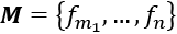 are features that are missing
- x is classified in y because F and M are true
One of the examples the authors of the publication describe in their paper is a classic example used to illustrate a decision-making process: estimating the health condition of a patient.
We will hence make use of the diagnosis process described in Chapter 1, Explaining Artificial Intelligence with Python, and in Chapter 3, Explaining Machine Learning with Facets.
In this section, we will expand the representations of these two chapters with contrastive explanations. We will explain how a missing feature can lead to the conclusion that a patient has a cold, the flu, pneumonia, or the West Nile virus.
We could, but will not, include the diagnosis of the COVID-19 2020 pandemic for ethical reasons. We cannot create an educational model representing a tragedy for humanity that is happening while writing this chapter. Let's go back to the case study in Chapter 1 and its initial dataset:
   colored_sputum  cough  fever  headache  class
0             1.0    3.5    9.4       3.0    flu
1             1.0    3.4    8.4       4.0    flu
2             1.0    3.3    7.3       3.0    flu
3             1.0    3.4    9.5       4.0    flu
4             1.0    2.0    8.0       3.5    flu
..            ...    ...    ...       ...    ...
145           0.0    1.0    4.2       2.3   cold
146           0.5    2.5    2.0       1.7   cold
147           0.0    1.0    3.2       2.0   cold
148           0.4    3.4    2.4       2.3   cold
149           0.0    1.0    3.1       1.8   cold
We will apply a contrastive explanation to the dataset to determine whether a patient has the flu or pneumonia. Examine these two sets of features for two instances of x to classify:
x1 = {cough, fever}
x2 = {cough, colored sputum, fever}
We will also add the number of days a patient has a fever with Facets as implemented in Chapter 3:

Figure 10.1: Facets representation of symptoms
The number of days is the x axis. If a patient has had a high fever for several days, a general practitioner will now have additional information. Let's add the number of days a patient has had a fever as the final feature of each instance:
x1 = {cough, fever, 5}
x2 = {cough, colored sputum, fever, 5}
We can now express the explanation of a doctor's diagnosis in CEM terms.
x1 most likely has the flu because feature {colored sputum) is absent, and {cough, fever, 5} are present.
x2 most likely has pneumonia because {Chicago}, one of the symptoms of the West Nile virus seen in Chapter 1, is absent, and {cough, colored sputum, fever, 5} are present. It must be noted that the West Nile virus can infect the patient without the colored sputum symptom.
We can sum CEM up as follows:
if FA absent and FP present, then prediction = True
In this section, we described contrastive explanations using text classification. In the next section and the remainder of this chapter, we will explore a Python program that explains images with CEM.
Getting started with the CEM applied to MNIST
In this section, we will install the modules and the dataset. The program will also prepare the data for the CNN model.
Open the CEM.ipynb program that we will use in this chapter.
We will begin by installing and importing the modules we need.
Installing Alibi and importing the modules
We will first install Alibi by trying to import Alibi:
# @title Install Alibi
try:
  import alibi
except:
  !pip install alibi
If Alibi is installed, the program will continue. However, when Colaboratory restarts, some libraries and variables are logs. In this case, the program will install Alibi.
We will now install the modules for the program.
Importing the modules and the dataset
In this section, we will import the necessary modules for this program. We will then import the data and display a sample.
Open the CEM.ipynb program that we will use in this chapter.
We will first import the modules.
Importing the modules
The program will import two types of modules: TensorFlow modules and the modules Alibi will use to display the explainer's output.
The TensorFlow modules include the Keras modules:
# @title Import modules
import tensorflow as tf
tf.logging.set_verbosity(tf.logging.ERROR) # suppress
                                           # deprecation messages
from tensorflow.keras import backend as K
from tensorflow.keras.layers import Conv2D, Dense, Dropout, Flatten, MaxPooling2D, Input, UpSampling2D
from tensorflow.keras.models import Model, load_model
from tensorflow.keras.utils import to_categorical
The Alibi explainer requires several modules for processing functions and displaying outputs:
import matplotlib
import matplotlib.pyplot as plt
import numpy as np
import os
from time import time
from alibi.explainers import CEM
We will now import the data and display a sample.
Importing the dataset
The program now imports the MNIST dataset. It splits the dataset into training data and test data:
# @title Load and prepare MNIST data
(x_train, y_train), (x_test, y_test) =
    tf.keras.datasets.mnist.load_data()
The dataset is now split and ready:
x_traincontains the training datay_traincontains the training data's labelsx_testcontains the test datay_testcontains the test data's labels
We will now print the shape of the training data and display a sample:
print('x_train shape:', x_train.shape, 'y_train shape:',
      y_train.shape)
plt.gray()
plt.imshow(x_test[15]);
The program first displays the shapes of the training data and its labels:
x_train shape: (60000, 28, 28) y_train shape: (60000,)
Then, the program displays a sample:

Figure 10.2: Displaying a CEM sample
The image is a grayscale image with values between [0, 255]. The values cover a wide range.
We will squash these values when we prepare the data.
Preparing the data
The data will now be scaled, shaped, and categorized. These phases will prepare the data for the CNN.
Scaling the data
The program first scales the data:
# @title Preparing data: scaling the data
x_train = x_train.astype('float32') / 255
x_test = x_test.astype('float32') / 255
print(x_test[1])
When we print the result of a sample, we will obtain squashed values in low dimensions that are sufficiently similar for the CNN to train and test its model:
[ 0.         0.         0.         0.         0.         0.
  0.         0.         0.68235296 0.99215686 0.99215686 0.99215686
  0.99215686 0.99215686 0.99215686 0.99215686 0.99215686 0.99215686
  0.99215686 0.99215686 0.9764706  0.96862745 0.96862745 0.6627451
  0.45882353 0.45882353 0.22352941 0.        ]
The original values of an image were in a [0, 255] range. However, when divided by 255, the values are now in a range of [0, 1].
Shaping the data
We still need to shape the data before sending it to a CNN:
# @title Preparing data: shaping the data
print("Initial Shape", x_test.shape)
x_train = np.reshape(x_train, x_train.shape + (1,))
x_test = np.reshape(x_test, x_test.shape + (1,))
print('x_train shape:', x_train.shape, 'x_test shape:', x_test.shape)
The output shows that a dimension has been added for the CNN:
Initial Shape (10000, 28, 28)
x_train shape:(60000, 28, 28, 1) x_test shape: (10000, 28, 28, 1)
We are almost ready to create the CNN model. We now have to categorize the data.
Categorizing the data
We need to categorize the data to train the CNN model:
# @title Preparing data: categorizing the data
y_train = to_categorical(y_train)
y_test = to_categorical(y_test)
print('y_train shape:', y_train.shape, 'y_test shape:', y_test.shape)
xmin, xmax = -.5, .5
x_train = ((x_train - x_train.min()) /
    (x_train.max() - x_train.min())) * (xmax - xmin) + xmin
x_test = ((x_test - x_test.min()) /
    (x_test.max() - x_test.min())) * (xmax - xmin) + xmin
The output now displays perfectly shaped data for the CNN model:
y_train shape: (60000, 10) y_test shape: (10000, 10)
We are now ready to define and train the CNN model.
Defining and training the CNN model
A CNN will take the input and transform the data into higher dimensions through several layers. Describing artificial intelligence, machine learning, and deep learning models is not within the scope of this book, which focuses on explainable AI.
However, before creating the CNN, let's define the general concepts that determine the type of layers it will contain:
- The convolutional layer applies random filters named kernels to the data; the data is multiplied by weights; the filters are optimized by the CNN weight optimizing function.
- The pooling layer groups features. If you have {1, 1, 1, 1, 1, ..., 1, 1, 1} in an area of the data, you can group them into a smaller representation such as {1, 1, 1}. You still know that a key feature of the image is {1}.
- The dropout layer literally drops some data out. If you have a blue sky with millions of pixels, you can easily take 50% of those pixels out and still know that the sky is blue.
- The flatten layer transforms the data into a long vector of numbers.
- The dense layer connects all the neurons.
Layer by layer, the CNN model will transform a large amount of data into a very high dimension of few values that represent the prediction as shown in the following output of the CNN model we are creating in this section:
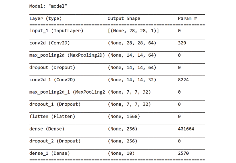
Figure 10.3: Structure representation of the model generated by TensorFlow
Let's now create the CNN model.
Creating the CNN model
We first create a function that adds the layers we described in the previous section to the model:
# @title Create and train CNN model
def cnn_model():
    x_in = Input(shape=(28, 28, 1))
    x = Conv2D(filters=64, kernel_size=2, padding='same',
               activation='relu')(x_in)
    x = MaxPooling2D(pool_size=2)(x)
    x = Dropout(0.3)(x)
    x = Conv2D(filters=32, kernel_size=2, padding='same',
               activation='relu')(x)
    x = MaxPooling2D(pool_size=2)(x)
    x = Dropout(0.3)(x)
    x = Flatten()(x)
    x = Dense(256, activation='relu')(x)
    x = Dropout(0.5)(x)
    x_out = Dense(10, activation='softmax')(x)
x_out contains the precious classification information we are looking for. The CNN model's function is called with the input data: inputs=x_in:
    cnn = Model(inputs=x_in, outputs=x_out)
    cnn.compile(loss='categorical_crossentropy', optimizer='adam',
                metrics=['accuracy'])
    return cnn
The model will be compiled and ready to be trained and tested.
Training the CNN model
Training the CNN model can take a few minutes. A form was added to skip the training process once the model has been saved:

Figure 10.4: CNN training options
The first time you run the program, you must set train_cnn to yes.
The CNN model will be called, trained, and saved in a file named mnist_cnn.h5:
train_cnn = 'no' # @param ["yes","no"]
if train_cnn == "yes":
  cnn = cnn_model()
  cnn.summary()
  cnn.fit(x_train, y_train, batch_size=64, epochs=3, verbose=0)
  cnn.save('mnist_cnn.h5')
cnn.summary() will display the structure of the CNN, as shown in the introduction of this section.
If you wish to keep this model and not have to train it each time you run the program, download it using the Colaboratory file manager.
First, click on the file manager icon on the left of the notebook's page:

Figure 10.5: File manager button
mnist_cnn.h5 will appear in the list of files:

Figure 10.6: List of temporary files
Right-click on mnist_cnn.h5 and download it.
When Colaboratory restarts, it deletes local variables. To upload the file to avoid training the CNN, upload the file by clicking on Upload:

Figure 10.7: Uploading the file
We will now load and test the accuracy of the model.
Loading and testing the accuracy of the model
The program trained and saved the CNN model in the previous cell of the program. It is now ready to be loaded and trained:
# @title Load and test accuracy on test dataset
cnn = load_model('/content/mnist_cnn.h5')
cnn.summary()
score = cnn.evaluate(x_test, y_test, verbose=0)
print('Test accuracy: ', score[1])
cnn.summary() displays the summary of the model and the test score:
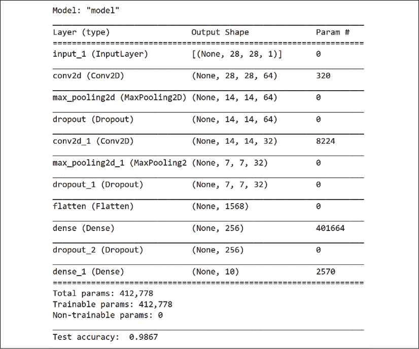
Figure 10.8: Summary of the model and test score
The test accuracy is excellent.
We will now define and train the autoencoder.
Defining and training the autoencoder
In this section, we will create, train, and test the autoencoder.
An autoencoder will encode the input data using a CNN with the same type of layers as the CNN we created in the Defining and training the CNN model section of this chapter.
However, there is a fundamental difference compared with the CNN:
An autoencoder encodes the data and then decodes the result to match the input data.
We are not trying to classify the inputs. We are finding a set of weights that guarantees that if we apply that set of weights to a perturbation of an image, we will remain close to the original.
The perturbations are ways to find the missing feature in an instance that produced a prediction. For example, in the The contrastive explanation method section of this chapter, we examined the following possible symptoms of the patient described as features:
Features for label 1 = {cough, fever, number of days=5}
The label of the diagnosis is flu.
The closest other label is pneumonia, with the following features:
Features for label 2 = {cough, colored sputum, fever, number of days=5}
Take a close look and see which feature is missing for the flu label.
For contrastive explanations, flu is pneumonia without colored sputum.
Perturbations will change the values of the features to find the missing feature—the pertinent negative (PN). If it finds a feature that would change a diagnosis if it were missing, it would be a pertinent positive (PP).
Alibi uses the autoencoder as an input to make sure that when the CEM explainer changes the values of the input to find the PN and PP features, it does not stray too far from the original values. It will stretch the input, but not much.
With this in mind, let's create the autoencoder.
Creating the autoencoder
The autoencoder is created in a function as described in the introduction of this section:
# @title Define and train autoencoder
def ae_model():
    x_in = Input(shape=(28, 28, 1))
    x = Conv2D(16, (3, 3), activation='relu', padding='same')(x_in)
    x = Conv2D(16, (3, 3), activation='relu', padding='same')(x)
    x = MaxPooling2D((2, 2), padding='same')(x)
    encoded = Conv2D(1, (3, 3), activation=None, padding='same')(x)

    x = Conv2D(16, (3, 3), activation='relu',
               padding='same')(encoded)
    x = UpSampling2D((2, 2))(x)
    x = Conv2D(16, (3, 3), activation='relu', padding='same')(x)
    decoded = Conv2D(1, (3, 3), activation=None, padding='same')(x)
    autoencoder = Model(x_in, decoded)
    autoencoder.compile(optimizer='adam', loss='mse')

    return autoencoder
The optimizer in the autoencoder guarantees that the output will match the input with a loss function that measures the distance between the original inputs and the weighted outputs.
We will visualize the outputs when we test the autoencoder.
Training and saving the autoencoder
In this section, we will train and save the autoencoder:
train_auto_encoder = 'no' # @param ["yes","no"]
if train_auto_encoder == "yes":
  ae = ae_model()
  # ae.summary()
  ae.fit(x_train, x_train, batch_size=128, epochs=4,
         validation_data=(x_test, x_test), verbose=0)
  ae.save('mnist_ae.h5', save_format='h5')
You can choose to train and save the autoencoder by selecting yes in the autoencoder form:

Figure 10.9: Autoencoder options
You can also select no in the form to skip the training phase of the autoencoder if you have already trained it. In that case, you download the mnist_ae.h5 file that has been created:

Figure 10.10: Saved autoencoder model
You can upload this file if you want to skip the training, as described in the Training the CNN model section of this chapter.
We will now load the autoencoder and visualize its performance.
Comparing the original images with the decoded images
In this section, we will load the model, display the summary, and compare the decoded images with the encoded ones:
First, we load the model and display the summary:
# @title Compare original with decoded images
ae = load_model('/content/mnist_ae.h5')
ae.summary()
The summary of the model is displayed:

Figure 10.11: Summary of the model generated by TensorFlow
The model now uses the autoencoder model to predict the output of an encoded image. "Predicting" in this case means reconstructing an image that is as close as possible to the original image:
decoded_imgs = ae.predict(x_test)
The decoded images are now plotted:
n = 5
plt.figure(figsize=(20, 4))
for i in range(1, n+1):
    # display original
    ax = plt.subplot(2, n, i)
    plt.imshow(x_test[i].reshape(28, 28))
    ax.get_xaxis().set_visible(False)
    ax.get_yaxis().set_visible(False)
    # display reconstruction
    ax = plt.subplot(2, n, i + n)
    plt.imshow(decoded_imgs[i].reshape(28, 28))
    ax.get_xaxis().set_visible(False)
    ax.get_yaxis().set_visible(False)
plt.show()
We first display the original images on the first line, and the second line shows the reconstructed images:

Figure 10.12: Controlling the output of the autoencoder
The autoencoder has been loaded and tested. Its accuracy has been visually confirmed.
Pertinent negatives
In this section, we will visualize the contrastive explanation for a pertinent negative.
For example, the number 3 could be an 8 with a missing half:

Figure 10.13: 3 is half of 8!
We first display a specific instance:
# @title Generate contrastive explanation with pertinent negative
# Explained instance
idx = 15
X = x_test[idx].reshape((1,) + x_test[idx].shape)
plt.imshow(X.reshape(28, 28));
The output is displayed as follows

Figure 10.14: An instance to explain
We now check the accuracy of the model:
# @title Model prediction
cnn.predict(X).argmax(), cnn.predict(X).max()
We can see that the prediction is correct:
(5, 0.9988611)
We will now create a pertinent negative explanation.
CEM parameters
We will now set the parameters of the CEM explainer.
The Alibi notebook explains each parameter in detail.
I formatted the code in the following text so that each line of code is preceded by the description of each parameter of Alibi's CEM open source function:
# @title CEM parameters
# 'PN' (pertinent negative) or 'PP' (pertinent positive):
mode = 'PN'
# instance shape
shape = (1,) + x_train.shape[1:]
# minimum difference needed between the prediction probability
# for the perturbed instance on the class predicted by the
# original instance and the max probability on the other classes
# in order for the first loss term to be minimized:
kappa = 0.
# weight of the L1 loss term:
beta = .1
# weight of the optional autoencoder loss term:
gamma = 100
# initial weight c of the loss term encouraging to predict a
# different class (PN) or the same class (PP) for the perturbed
# instance compared to the original instance to be explained:
c_init = 1.
# nb of updates for c:
c_steps = 10
# nb of iterations per value of c:
max_iterations = 1000
# feature range for the perturbed instance:
feature_range = (x_train.min(),x_train.max())
# gradient clipping:
clip = (-1000.,1000.)
# initial learning rate:
lr = 1e-2
# a value, float or feature-wise, which can be seen as containing
# no info to make a prediction
# perturbations towards this value means removing features, and
# away means adding features for our MNIST images,
# the background (-0.5) is the least informative, so
# positive/negative perturbations imply adding/removing features:
no_info_val = -1.
We can now initialize the CEM explainer with these parameters.
Initializing the CEM explainer
We will now initialize the CEM explainer and explain the instance. Once you understand this set of parameters, you will be able to explore other scenarios if necessary.
First, we initialize the CEM with the parameters defined in the previous section:
# @title initialize CEM explainer and explain instance
cem = CEM(cnn, mode, shape, kappa=kappa, beta=beta,
          feature_range=feature_range,gamma=gamma, ae_model=ae,
          max_iterations=max_iterations, c_init=c_init,
          c_steps=c_steps, learning_rate_init=lr, clip=clip,
          no_info_val=no_info_val)
Then, we create the explanation:
explanation = cem.explain(X)
We will now observe the visual explanation provided by the CEM explainer.
Pertinent negative explanations
The innovative CEM explainer provides a visual explanation:
# @title Pertinent negative
print('Pertinent negative prediction: {}'.format(
      explanation.PN_pred))
plt.imshow(explanation.PN.reshape(28, 28));
It shows the pertinent negative prediction, that is, portions of 3:

Figure 10.15: Explaining a PN
Pertinent positive explanations are displayed in the same way. You may notice that images are sometimes fuzzy and noisy. That is what is going on inside the inner workings of machine learning and deep learning! The CEM explainer runs in a cell and produces an explanation for a pertinent positive instance:
# @title Pertinent positive
print('Pertinent positive prediction: {}'.format(
      explanation.PP_pred))
plt.imshow(explanation.PP.reshape(28, 28));
The pertinent positive explanation is displayed:

Figure 10.16: Explaining PP
We can see that the image obtained vaguely resembles the number 5.
In this section, we visualized CEM explanations and can reach the following conclusions:
- A prediction can be made by removing features to explain a prediction. This is a pertinent negative (PN) approach. For example, you can, depending on the font, describe the number 3 as the number 8 with a missing half. The opposite can be true leaning to the pertinent positive (PP) approach.
- When making perturbations in inputs to reach a PN, we remove features.
- When making perturbations in inputs to reach a PP, we add features.
- For example, adding and removing information can be done by removing a white (replaced by black) pixel or by adding a white pixel.
- The perturbations are made without any knowledge of the model's prediction.
The CME adds another tool to your explainable AI toolkit with its innovative missing feature approach.
Summary
In this chapter, we learned how to explain AI with human-like reasoning. A bank will grant a loan to a person because their credit card debt is non-existent or low. A consumer might buy a soda because it advertises low sugar levels.
We found how the CEM can interpret a medical diagnosis. This example expanded our representation of the XAI process described in Chapter 1, Explaining Artificial Intelligence with Python.
We then explored a Python program that explained how predictions were reached on the MNIST dataset. Numerous machine learning programs have used MNIST. The CEM's innovative approach explained how the number 5, for example, could be predicted because it lacked features that a 3 or an 8 contain.
We created a CNN, trained it, saved it, and tested it. We also created an autoencoder, trained it, saved it, and tested it.
Finally, we created a CEM explainer that displayed PNs and PPs.
Contrastive explanations shed new light on explainable AI. At first, the method seems counter-intuitive. XAI tools usually explain the critical features that lead to a prediction.
The CEM does the opposite. Yet, human decisions are often based on a missing feature as represented. Many times, a human will say, it cannot be x, because there is no y.
We can see that XAI tools will continue to add human reasoning to help a user relate to AI and understand a model's predictions.
In the next chapter, Anchors XAI, we will add more human reasoning to machine learning explanations.
Questions
- Contrastive explanations focus on the features with the highest values that lead to a prediction. (True|False)
- General practitioners never use contrastive reasoning to evaluate a patient. (True|False)
- Humans reason with contrastive methods. (True|False)
- An image cannot be explained with CEM. (True|False)
- You can explain a tripod using a missing feature of a table. (True|False)
- A CNN generates good results on the MNIST dataset. (True|False)
- A pertinent negative explains how a model makes a prediction with a missing feature. (True|False)
- CEM does not apply to text classification. (True|False)
- The CEM explainer can produce visual explanations. (True|False)
References
- Reference code for the CEM: https://docs.seldon.io/projects/alibi/en/stable/examples/cem_mnist.html
- Reference documents for the CEM: https://docs.seldon.io/projects/alibi/en/stable/methods/CEM.html
- Contrastive Explanations Help AI Explain Itself by Identifying What Is Missing (Amit Dhurandhar): https://www.ibm.com/blogs/research/2018/05/contrastive-explanations/
Further reading
For more on the CEM:
- Explanations Based on the Missing: Toward Contrastive Explanations with Pertinent Negatives, by Amit Dhurandhar, Pin-Yu Chen, Ronny Luss, Chun-Chen Tu, Paishun Ting, Karthikeyan Shanmugam, and Payel Das: https://arxiv.org/abs/1802.07623
- The AI Explainability 360 toolkit contains the definitive implementation of the contrastive explanations method, and can be found at http://aix360.mybluemix.net/