12.1. SQL: Relational Algebra
So far we’ve seen how to design a conceptual schema and map it to a relational schema. The relational schema may now be implemented in a relational DBMS, and its tables populated with data. To retrieve information from the resulting database, we need to issue queries. In practice the most popular query languages are SQL (popularly, if incorrectly, called “Structured Query Language”) and QBE (Query By Example). Both of these are based, at least partly, on a formal query language known as relational algebra, which is discussed in this section. Studying this algebra first clarifies the basic query operations without getting distracted by the specific syntax of commercial query languages.
With the algebra under our belt, we will be able define what is really meant by the term “relational database system”. The following sections then cover SQL in some depth, starting with the basics and moving on through intermediate to advanced concepts. Although our focus is on the SQL standard(s), some additional details will be included about commercial dialects of SQL. Now let’s begin with relational algebra.
In the relational model of data, all facts are stored in tables (or relations). New tables may be formed from existing tables by applying operations in the relational algebra. The tables resulting from these operations may be named and stored, using relational assignment. The original relational algebra defined by Codd contained eight relational operators: four based on traditional set operations (union, intersection, difference, and Cartesian product) and four special operations (selection, projection, join, and division). Each of these eight relational operators is a table-forming operator on tables. For example, the union of two tables is itself a table.
Relational algebra includes six comparison operators (=, <>, <, >, <=, >=). These are proposition-forming operators on terms. For example, x <> 0 asserts that x is not equal to zero. It also includes three logical operators (and, or, not). These are proposition-forming operators on propositions (e.g., x > 0 and x < 8). Since the algebra does not include arithmetic operators (e.g., +) or functions (e.g., count), it is less expressive than SQL. Proposed extensions to the algebra to include these and other operators are ignored here.
Many different notations exist for expressing the relational algebra. A comparison between our notation and a common academic notation is given later. To simplify discussion, we’ll often use informal terms instead of the strict relational terminology (e.g., “table” and “row” instead of “relation” and “tuple”).
Union, Intersection, and Difference
Two tables are union compatible if and only if they have the same number of columns and their corresponding columns are based on the same domain (the columns may have different names). Treating a table as a set of rows, the traditional set operations of union, intersection, and difference may be defined between tables that are union compatible.
Consider the conceptual schema in Figure 12.1. In this small UoD, people are identified by their first name. We record facts about the foods that people eat, and about the foods that they like. The relational schema comprises two tables as shown. The populations of the tables may properly overlap or even be disjoint. Hence there are no intertable constraints in the relational schema—this situation is fairly unusual.
Figure 12.1. The conceptual schema maps to two tables.

Figure 12.2 includes sample data. The union of tables A and B is the set of all rows belonging to A or B (or both). We write this as “A ∪ B” or “A union B”. Suppose that we want to pair each person up with foods that they either eat or like. This may be specified simply as the union of the tables, Eats ∪ Likes. Figure 12.2 includes this query expression and the resulting (unnamed) table, which includes all the rows in the Eats table as well as all the rows in the Likes table. As with any table, duplicate rows are excluded, so rows in both the Eats and the Likes tables appear only once in the result.
Figure 12.2. The union of two tables is the set of rows that occur in either table (or both).

Note that “Eats ∪ Likes” is an expression describing how the result may be derived in terms of tables stored in the database (i.e., base tables): it is not a table name. We may refer to a query result as a result table, answer table, or derived table. The order of the rows in the tables has no significance, since we are dealing with sets. Actual query languages such as SQL provide ways to display rows in any preferred order.
The intersection of tables A and B is the set of rows common to A and B. We write this as “A ∩ B” or “A intersect B”. For instance, to list facts about foods that people both eat and like, we may specify this as the intersection of our two base tables, Eats ∩ Likes (see Figure 12.3).
Figure 12.3. The intersection of two tables is the set of rows common to both.

We define the difference operation between tables thus. A - B is the set of rows belonging to A but not B. We may also write this as A minus B, or A except B. For example, the expression Eats - Likes returns details about people who eat foods they don’t like (see Figure 12.4(a)).

As in ordinary set theory, the union operation is commutative (i.e., the order of the operands is not significant). So, given any tables A and B it is true that A ∪ B = B ∪ A. Likewise, the intersection operation is commutative, i.e., A ∩ B = B ∩ A. The difference operation, however, is not commutative so it is possible that A - B does not equal B- A. For example, Likes - Eats returns facts about who likes a food but doesn’t eat it (see Figure 12.4(b)). Compare this with the previous result.
Cartesian Product (Unrestricted Join)
In mathematics, the Cartesian Product of sets A and B is defined as the set of all ordered pairs (x, y) such that x belongs to A and y belongs to B. For example, if A = {1, 2} and B ={3, 4, 5}, then the Cartesian Product of A and B is {(1, 3), (1, 4), (1,5), (2, 3), (2, 4), (2, 5)}. We write this product as A × B (read “A cross B”). This definition applies also to tables, although the ordered pairs of rows (x, y) are considered to be single rows of the product table, which inherits the corresponding column names. Thus if A and B are tables, A × B is formed by pairing each row of A with each row of B. Here “pairing with” means “prepending to”. The expression “A × B” may also be written as “A times B”. The Cartesian product is also called the “cross join” or “unrestricted join”.
Since A × B pairs each row of A with all rows of B, if A has n rows and B has m rows, then the table A × B has n × m rows. So the number of rows in A × B is the product of the number of rows in A and B. Since the paired rows are concatenated into single rows, the number of columns in A × B is the sum of the number of columns in A andB.
Let’s look at a simple example. In Figure 12.5, A is a 3 × 2 table (i.e., 3 rows × 2 columns) and B is a 2 × 1 table. So A × B has six (3 × 2) rows of three (2 + 1) columns. The header rows that contain the column names al, a2, bl are not counted in this calculation. In this example, dotted lines have been ruled between rows to aid readability. Note that the Cartesian Product A × B exists for any tables A and B; it is not necessary that A and B be union compatible.
Figure 12.5. A × B pairs each row of A with each row of B.

If we define Cartesian products in terms of tuples treated as ordered sequences of values, the × operator is not commutative (i.e., A × B need not equal B × A). This is the usual treatment in mathematics. With relational databases, however, each column has a unique name, so a tuple may instead be treated as an (unordered) set of attribute-value pairs (each value in a row is associated with its column name). In this sense, columns are said to be “ordered by name”. With this view of tuples, the × operator is commutative.
To clarify this, compute B × A for the example in Figure 12.5. Although the resulting table has its columns displayed in the order bl, al, a.2, and the values are ordered accordingly, the information is the same as for A × B, since each value can be linked to its column name. For example, the first row of B × A may be represented as {(bl, 7), (al, 1), (a2, 2)}, which equals {(al, 1), (a2, 2), (bl, 7)}, which represents the first row of A × R Once columns are uniquely named, their physical order has no semantic significance.
As in standard set theory, the operations of union, intersection, and Cartesian product are associative. For instance, A ∪ (B ∪ C) = (A ∪ B) ∪ C. Since no ambiguity results, parentheses may be dropped in such cases. For example, the expression “A ∪ B ∪ C” is permitted. Of the four table operations considered so far, difference is the only one that is not associative; that is, it is possible that A - (B- C) is not equal to (A - B)- C. As an exercise, use Venn diagrams to check these claims.
Recall that column names of a table must be unique. If A and B have no column names in common, then A × B uses the simple column names of A and B. If A and B are different but have some common column names, the corresponding columns in A × B are uniquely referenced by using qualified names (with the prefix “A.” or ”B”). However, what if A and B are the same (i.e., we wish to form the Cartesian product of a table with itself)?
Consider the Person × Person table in Figure 12.6. This breaks the rule that column names in a table must be unique. In this case, simply using the qualified column names will not solve the problem either because we would have two columns named “Person.firstname” and two columns named “Person.gender”.
Figure 12.6. What is wrong with this Cartesian product?

This problem is overcome by introducing aliases for tables. For example, we could use “Person2” as an alternative name for the table and form the product as shown in Figure 12.7. If desired, we could have introduced two aliases, “Person1” and “Person2”, to specify the product Person1 × Person2. The need to multiply a table by itself may arise if we have to compare values on different rows. Aliases can also be used simply to save writing (by introducing shorter names).
Figure 12.7. Table aliases are needed to multiply a table by itself.

Relational Selection
Let us now consider the four table operations introduced by Codd. The first of these is known as selection (or restriction). Don’t confuse this with SQL’s select command.
In relational algebra, the selection operation chooses just those rows that satisfy a specified condition. Visually we can picture the operation as returning a horizontal or row subset, since it returns zero or more rows from the original table (see Figure 12.8).
Figure 12.8. The selection operation in relational algebra.

The selection operation may be specified using an expression of the form T where c. Here T denotes a table expression (i.e., an expression whose value is a table) and c denotes a condition. The selection operation returns just those rows where the condition evaluates to True, filtering out rows where the condition evaluates to False or Unknown. The “where c” part is called a where clause. This notation encourages top-down thinking (find the relevant tables before worrying about the rows) and agrees with SQL syntax. The alternative notation σc(T) is often used in academic journals. The “σ” is sigma, the Greek “s” (which is the first letter of “selection”).
In Figure 12.9, the Player table stores details about tennis players. To list details about just the male tennis players, we could formulate this selection as indicated, giving the result shown. Here the selection condition is just the equality: gender = ‘M’. The use of single quotes with ‘M’ indicates that this value is literally the character ‘M’. Single quotes are also used when referencing character string values such as ‘David’. Numeric values should not be quoted. Although the table resulting from the selection is unnamed, its columns have the same names as the original.
Figure 12.9. The selection operation picks those rows that satisfy the condition.

The condition c may contain any of six comparison operators:= (equals); < > (is not equal to); < (is less than); > (is greater than); <= (is less than or equal to); and >= (is greater than or equal to). Sometimes the result of a table operation is an empty table (cf. the null set). For instance, no rows satisfy the condition in Player where height > 180.
If conditions do not involve comparisons with null values, they are Boolean expressions—they evaluate to True or False. If conditions do include comparisons with nulls, a three-valued logic is used instead, so that the condition may evaluate to True, False, or Unknown. This is also what happens in SQL. In either case, the selection operation returns just those rows where the condition is true. Any row where the condition evaluates to false or unknown is filtered out.
In addition to comparison operators, conditions may include three logical operators: and, or, not. As usual, or is inclusive. As an exercise, formulate a query to list details of those females who are shorter than 170 cm. Refer to the Player table and see if you can state the result, and then check your answer with Figure 12.10. To aid readability, reserved words are in bold.
Figure 12.10. Are the parentheses needed in this query?

The query in Figure 12.10 used parentheses to clarify the order in which operations are to be carried out. With complicated expressions, however, large numbers of parentheses can make things look very messy (cf. LISP). Unlike several programming languages (e.g., Pascal), most query languages (e.g., SQL) give comparison operators higher priority than logical operators. So the operators =, <>, <, >, < =, >= are given precedence over not, and, and or for evaluation purposes. We make the same choice in relational algebra since this reduces the number of parentheses needed for complex expressions. With this understood, the query in Figure 12.10 may be rewritten more concisely as:
Player where gender = ‘F’ and height < 170
To further reduce the need for parentheses, the algebra adopts the logical operator priority convention commonly used in computing languages, such as Pascal and SQL. First evaluate not, then and, and then or. Table 12.1 shows the evaluation order for both comparison and logical operators. This operator precedence may be overridden by the use of parentheses.
| Priority | Operators |
|---|---|
| 1 | =, <>, <, >, < =, > = |
| 2 | not |
| 3 | and |
| 4 | or |
For example, suppose we want details about males who are taller than 175 cm or shorter than 170 cm. The query in Figure 12.11(a) looks like it should work for this, but the wrong result is obtained. Why?
Figure 12.11. Unless parentheses are used, and is evaluated before or.

Because the and operator is evaluated before the or, this query is interpreted as Player where (gender = ‘M’ and height > 175) or height < 170. Notice that line breaks have no significance to the meaning of the query. So the result includes details about anybody shorter than 170 cm (including females). The query in Figure 12.11(b) corrects this by including parentheses around the height disjunction to evaluate the or operator before the and operator.
To obtain details about players who are either males over 175 cm or females at least 170 cm tall, either of the queries shown in Figure 12.12 may be used. In the query in Figure 12.12(b), parentheses are redundant since the and operators are evaluated before the or operator anyway. If in doubt about whether parentheses are needed, put them in.
Figure 12.12. Two equivalent queries; if in doubt, include parentheses.

Figure 12.13 shows three equivalent queries for listing information on players who are neither taller than 172 cm nor shorter than 168 cm. Operator precedence ensures that query (a) in Figure 12.13 means Player where (not (height > 172)) and (not (height < 168)). Note that the six comparison operators may be grouped into three pairs of opposites: =, <>; <, > = ; and >, < = . So the query in Figure 12.13(a) may be replaced by the shorter query in Figure 12.13(b).
Figure 12.13. Three equivalent queries.

De Morgan’s laws, named after the famous logician Augustus De Morgan, are the following:
not (p and q) = not p or not q
not (p or q) = not p and not q
Here p and q denote any proposition or logical condition. These laws hold in both two-valued and three-valued logic, so are safe to use with null values. Using the second of these laws, it is easy to see that the query in Figure 12.13(c) is equivalent to the query in Figure 12.13(a).
Relational Projection
The next table operation, known as projection, was introduced in Chapter 4. This operation involves choosing one or more columns from a table and then eliminating any duplicate rows that might result. It is said to produce a vertical subset or column subset. Figure 12.14 illustrates a projection on two columns.
Figure 12.14. The projection operation in relational algebra.

We may represent the projection operation as T [a,b,...] where T is a table expression and a, b,... are the names of the required columns (this column list is called the projection list). To delimit the projection list we use square brackets rather than parentheses, since the latter have other uses in queries (e.g., to change the evaluation order of operations). Italicizing the square brackets “[ ]” helps distinguish them from the use of “[ ]” to delimit optional items, or bags, and to indicate an extra task (duplicate elimination) once the columns are chosen.
The alternative notation πa,b...(T) is common in academic journals. The “π” symbol is pi, the Greek “p” (the first letter of “projection”). Like SQL, this notation lists the required columns before the tables. Our preferred notation instead encourages top-down thinking by identifying the relevant tables before listing the columns.
Figure 12.15 gives two examples, based on the table Player( name, gender, height). When projecting on a single base table, if the chosen columns include a candidate key then no duplicates rows can result. If not, duplicates may arise. For example, choosing just the gender column gives the bag [‘M’, ‘F’, ‘F’, ‘M’]. To complete the projection the duplicate values are eliminated, giving the set {‘M’, ‘F’}. If we project on all columns, we end up with the same table. For instance, Player [name, gender, height] is the same table as Player.
Figure 12.15. Projection involves picking the columns and removing any duplicates

The same column must not be mentioned twice in a projection. For example, Player [name, name] is illegal (why?). If desired, projection may be used to display columns in a different order. For example, Player [height, gender, name] reverses the order. Since unique column names are listed in the result, this doesn’t change the meaning.
If the relational schema is fully normalized, it is fairly unusual to have base tables that are union compatible (the Eats and Likes tables considered earlier being an exception). So the ∪, ∩, and - operations tend to be used almost exclusively with result tables that have become union compatible because of projections.
Let’s look now at some examples that are a little more difficult. To facilitate a discussion of a step-by-step approach to such cases, we’ll use the relational assignment operation. Because their contents may vary, table schemes may be regarded as variables. In fact, tables are the only kind of variable allowed in relational algebra. The notion of relational assignment, which is strictly separate from the algebra itself, is similar to that in programming languages. Using the symbol “:=” for “becomes” or “is assigned the value of, we may write assignment statements of the form
table variable := table expression
This is an instruction to first evaluate the expression on the right, and then place its value in the variable named on the left. If this variable had a previous value, the old value would simply be replaced by the new value. For example, if X, A, and B are table values, then the statement “X := A – B” means X is assigned the value of A - B.
Once named in a relational assignment, result tables may be used just like base tables in later expressions. For example, to store details about male tall players in a table called “MaleTallPlayer”, we could make the following three assignments. To list these details, our query is simply the table name MaleTallPlayer.
MalePlayer := Player where gender = ‘M’
TallPlayer := Player where height > 175
MaleTallPlayer := MalePlayer ∩ TallPlayer
As a more difficult example, consider the UoD of Figure 12.16. How may we formulate this query in relational algebra: Which non-European countries speak French? Try this yourself before reading on.
Figure 12.16. Conceptual and relational schemas, with sample population.

We could formulate the query in steps, using intermediate tables on the way to obtaining our final result table. For example:
NonEuroCountry := (Location where region <> ‘Europe’) [country]
FrenchSpkCountry := (Spokenln where language = ‘French’) [country]
FrenchSpkNonEuroCountry := NonEuroCountry ∩ FrenchSpkCountry
Here our first step was to find the non-European countries: {Australia, Canada}. Then we found the French-speaking countries: {Belgium, Canada, France}. Finally we took the intersection of these, giving the result: {Canada}.
Setting queries out this way is known as stepwise formulation. Doing things in stages can sometimes make it easier to formulate difficult queries. However, it saves writing to express a query by means of a single expression. For instance, the three assignment statements just considered can be replaced by
(Location where region <> ‘Europe’) [country]
∩
(Spokenln where language = ‘French’) [country]
This lengthy expression is said to be a nested formulation because it nests one or more queries inside another. For complex queries we might perform the stepwise formulation in our heads, or scribbled down somewhere, and then convert this into the nested formulation. In general, any information capable of being extracted by a series of relational algebra queries can be specified in a single relational algebra query.
Note that projection does not distribute over intersection. In other words, given tables A and B, and a projection list p, it is possible that (A ∩ B)[p] ≠ A[p] ∩ B[p]. For instance, the following query is not equivalent to the previous one (why not?).
((Location where region <> ‘Europe’) ∩ (Spokenln where language = ‘French’)) [country]
This query is illegal, since the table operands of ∩ are not compatible. Even if A and B are compatible, projection need not distribute over ∩ or over –. If A and B are compatible, projection does distribute over ∪, i.e., (A ∪ B)[p] = A[p] ∪ B[p]. As an exercise, you may wish to prove these results.
Relational Joins
Object joins at the conceptual level were introduced in Section 4.4 to help clarify the meaning of external uniqueness constraints. We now consider the relational join operation between two tables (or two occurrences of the same table), which compares attribute values from the tables, using the comparison operators (=, <, >, <>, < =, >=). There are several kinds of join operations, and we discuss only some of these here. Columns being compared in any join operation must be defined on the same domain; they do not need to have the same name. Where it is necessary to distinguish between join columns with the same local name, we use their fully qualified names.
Let ⊖ (theta) denote any comparison operator (=, < etc.). Then the ⊖-join of tables A and B on attributes a of A and b of B equals the Cartesian product A × B, restricted to those rows where A.a ⊖ B.b. We write this as shown here. An alternative, academic notation is shown in braces.
(A × B) where c { or A ⋈c B }
The condition c used to express this comparison of attributes between tables is called the join condition. The join condition may be composite (e.g., a1 < b1 and a2 < b2). Because of the Cartesian product, the resulting table has a number of columns equal to the sum of the number of columns in A and B, but because of the selection operation, it typically has far fewer rows than the product of the numbers of rows of the joined tables.
With most joins, the comparison operator used is =. The ⊖-join is then called an equijoin. Thus the equijoin of A and B equating values in column a of A with column b of B is A × B restricted to the rows where A.a = B.b. If the join column names are different in each table, there is no need to qualify them with table names. We write this as shown here. In general, the join condition may contain many equalities.
(A × B) where A.a = B.b
or
(A × B) where a = b {if a, b occur in only one of A, B}
Let’s consider an example. Figure 12.17.includes a simple conceptual schema and its corresponding relational schema. A sample population is given in Figure 12.18.
Figure 12.17. The ORM schema (a) maps to the relational schema (b).

Figure 12.18. A sample population for the schema in Figure 12.17.

Before formulating queries you should familiarize yourself with the structure and contents of the database. From the schema, we see that employees are identified by their employee number, and their name and gender must also be recorded. An employee may drive many cars, and the same car may be driven by many employees. The population is not significant, since it does not include instances where the same name applies to more than one employee. However, it does illustrate that driving cars is optional (employees 002 and 004), that an employee may drive more than one car (employee 003), and that the same car may be driven by more than one employee (car ABC 123). Now consider the following query: “List the employee number, name, and cars for each employee who drives a car”.
We could specify this by the equijoin in Figure 12.19, which joins the tables by equating their empNr attributes. To help explain this, dotted lines have been added between the base tables to indicate which rows match on their empNr value. Only the first and third rows from the Employee table are able to find a match. The third row (003) finds two matches. Check the result for yourself.
Figure 12.19. An equijoin.

Because the join columns here have the same local name, “empNr”, qualified names are used to distinguish the columns in the query and the join result. The join columns don’t have to have the same (unqualified) name—as long as they belong to the same domain, the join can be made. For example, if the employee number column in the Drives table was named “empld”, the join condition could be specified as “empNr = empld”.
As this example illustrates, an equijoin contains two matching columns resulting from each join attribute (note the two empNr columns). If these columns actually refer to the same thing in the UoD (and they typically do), then one of these columns is redundant. In this case, we lose no information if we delete one of these matching columns (by performing a projection on all but the column to be deleted). This is done in Figure 12.20.
Figure 12.20. The duplicate column is removed by projection on the equijoin.

If the columns used for joining have the same name in both tables, then the unqualified name is used in the join result. The resulting table is then said to be the natural inner join of the original tables. Since “inner” is assumed by default, the natural inner join may be expressed simply as natural join (outer joins are discussed later). This is by far the most common join operation in practice. The natural join of tables A and B may be written as A ⋈ B, or in words as “A natural join B”. This may be summarized as follows.
| To compute A ⋈ B: | Form A × B |
For each column name c that occurs in both A and B
|
There is no need to name the join columns because these are the ones with the same names in both tables (and of course these must be based on the same domain). To help remember the bow-tie “⋈” notation, note that “⋈” looks like a cross “×” with two vertical lines added, suggesting that a natural join is a Cartesian product plus two other operations (selection of rows with equal values for the common columns, followed by projection to delete redundant columns). Figure 12.21 shows the natural join for our driving example. Note that the empNr column appears just once and is unqualified.
Figure 12.21. A natural join.

If the tables have no column names in common, then the natural join is simply the Cartesian product. Like the Cartesian product, natural join is associative: (A ⋈ B) ⋈ C = A ⋈ (B ⋈ C). So expressions of the form A ⋈ B ⋈ C are unambiguous.
Tables being joined may have zero, one, or more common columns. In any case, the natural join is restricted to those rows where all the common attributes have the same value in both tables. The number of columns in A ⋈ B equals the sum of the number of columns in A and B, minus the number of columns common to both.
To illustrate a natural join on many attributes, consider the UoD in Figure 12.22. First examine the conceptual schema. Within a bank branch, an account may be identified by its local account number. But different accounts in different branches may have the same local account number. So, globally, the bank identifies accounts by a combination of branch and account number. Clients are identified by a global client number and have a name (not necessarily unique). Not all clients need an account. The relational schema is included in Figure 12.22.
Figure 12.22. Account has a composite identification scheme.

Notice the subset and equality constraints between the tables shown in Figure 12.22. Joins are usually, although not always, made across such constraint links. Simple joins may be performed on clienfNr, and composite joins on branchNr-accountNr pairs (which identify accounts). Figure 12.23 shows sample data.
Figure 12.23. Sample population for the bank schema.

The two queries in Figure 12.24 use natural joins to display users and balances of accounts. The first query matches accounts by joining on both branchNr and accountNr. To add client names, the second query also matches clients by joining on clientNr.
Figure 12.24. Two queries using natural joins.

In rare cases, comparison operators other than equality are used in joins. As a simple example, consider the Drinker and Smoker tables in Figure 12.25. These might result from a decision to map subtypes of Patient to separate tables.
Figure 12.25. Example of a <>-join.

Suppose we wanted a list of drinker, smoker pairs, where the drinker and smoker are distinct persons. This can be formulated by a <>-join as shown. Here the comparison operator is “<>”. Notice that because drinkers and smokers overlap, some patient doubles may appear twice (in different order). Similarly, <-joins, >-joins, <=-joins and >=-joins may be defined.
The kinds of joins discussed so far are collectively known as inner joins. We can also have outer joins, which are used to include various cases with null values. An outer join is basically an inner join, with extra rows padded with nulls when the join condition is not satisfied. For example, given the data population shown in Figure 12.23, the result of Client left outer join AcUser includes a row to indicate that client 8005 has the name “Shankara TA” but uses no account (branchNr and accountNr are null on this row). The left outer join includes all the clients from the left-hand table (i.e., the table on the left of the join operator), whether or not they are listed in the right-hand table. Outer joins are discussed in detail later for SQL.
Relational Division
The final relational operation we consider is relational division. Division of table A by table B is only meaningful if A has more columns than B. Let’s assume that table A has two sets of columns, X and Y, and table B has a set of columns Y. In other words, X is the set of columns in A that are not present in B. We’ll assume an ordered relation between the Y columns in A and B so that we know which column in B corresponds to which column in A.
The result of A ÷ B is formed by restricting the result to those rows of A where the Y column values in A all the rows of B and then deleting the Y columns from A. The expression A ÷ B may also be written as A divide-by B. Figure 12.26 shows a trivial example, where the attribute domains are denoted by XI, X2, Yl.
Figure 12.26. A simple example used to explain relational division.

Although not used very often, the division operation can be useful in listing rows that are associated with at least all rows of another table expression (e.g., who can supply all the items on our stock list?).
As a practical example, suppose the table Speaks ( country, language) stores facts about which countries speak (i.e., use) which languages. A sample population is shown in the large table within Figure 12.27. Now consider the query: Which countries speak all the languages spoken in Canada? To answer this, we first find all the languages spoken in Canada, using the expression Speaks where country = ‘Canada’ [language]. This returns the table {English, French}. We then divide the Speaks table by this result, as shown, to obtain the final answer {Canada, Dominica).
Figure 12.27. A practical example of relational division.

Query Strategies
That completes all the main operators in relational algebra. Table 12.2 indicates the operator precedence adopted in this book. The comparison operators have top (and equal) priority, so are evaluated first. Next the logical operators are evaluated (first not, then and, then or). Then relational selection and projection are evaluated (equal priority). Finally the other six relational operators (union, intersection, difference, Cartesian product, natural join, and division) are evaluated (equal priority). Operators with equal priority are evaluated left to right. Expressions in parentheses are evaluated first. Some systems adopt a different priority convention for the relational operators.
| Priority | Operator type | Operator(s) |
|---|---|---|
| 1 | Comparison | =, <>, <, >, <=, > = |
| 2 | Logical | not |
| 3 | and | |
| 4 | or | |
| 5 | Relational | selection (... where ...), projection ...[ a, b] |
| 6 | ∩ ∪ – × ⋈ ÷ |
To help formulate queries in relational algebra, the following query strategies are useful:
Phrase the query in natural language, and understand what it means.
Ask which tables hold the information.
If you have table data, answer the query yourself and then retrace your mental steps.
Divide the query up into steps or subproblems.
If the columns to be listed are in different tables, declare joins between the tables.
If you need to relate two rows of the same table, use an alias to perform a self-join.
Our first move is to formulate the query in natural language, ensuring that we understand what the query means. Next determine what tables hold the information needed to answer our query. The information might be in a single table or be spread over two or more tables. If the columns to be listed come from different tables (or different copies of the same table), then we must normally specify joins between these tables. These joins might be of any kind: inner or outer joins, natural or theta joins, or cross joins (Cartesian products).
Apart from some cases involving ∪, ∩, or -, relational algebra requires joins whenever different tables must be accessed to determine the result, even if the result columns come from the same table. SQL introduced subqueries, which can be used instead of joins when the result columns come from the same table.
Let’s look at an example using our bank account database. To reduce page turning, the database is reproduced in Figure 12.28. Now consider the query: Which clients have an account with a balance of more than $700? Before formulating this in relational algebra, we should ensure that we understand what the natural language query means. In some cases we may need to clarify the meaning by asking the person who originally posed the query. For example, do we want just the client number for the relevant clients or do we want their name as well? Let’s assume that we want the client name as well. Looking at the tables, we can now see that all three tables are needed. The Account table holds the balances, the Client table holds the client names, and the AcUser table indicates who uses what account.
Figure 12.28. How can this query be formulated in relational algebra?

Since we have sample data, we can first try to answer the English query, examine what we did, and finally try to express this in the formal language of relational algebra. If we were answering the request ourselves, we might go to the Account table and select just the rows where the balance exceeded $700. This yields the account (10, 54) and the account (23, 54). We might then look at the AcUser table to see who uses these accounts. This yields the clients numbered 1001, 1002, and 7654. Now we look to the Client table to find out their names (‘Jones, ME’, ‘Jones, TA’, ‘Seldon, H’). So our answer is {(1001, ‘Jones, ME’), (1002, ‘Jones, TA’), (7654, ‘Seldon, H’)}.
Retracing and generalizing our steps, we see that we joined the Account and AcUser tables by matching the account (branchNr and accountNr), and we linked with the Client table by joining on clientNr. Since these attributes have the same names over the tables, we can use natural joins. We may set this out in relational algebra as
(Account where balance > 700) [ branchNr, accountNr]
⋈ AcUser
⋈ Client [ clientNr, clientName]
This isn’t the only way we could express the query. For instance, using a top-down approach, both joins could have been done before selecting or projecting, thus:
(Account ⋈ AcUser ⋈ Client)
where balance > 700
[ clientNr, clientName]
Notice how queries may be spread over many lines to make them more readable. A useful syntax check is to ensure that you have the same number of opening and closing brackets. Although these two queries are logically equivalent, if executed in the evaluation order shown, the second query is less efficient because it involves a larger join. Relational algebra can be used to specify transformation rules between equivalent queries to obtain an optimally efficient, or at least a more efficient, formulation. SQL database systems include a query optimizer to translate queries into an optimized form before executing them. So in practice we often formulate queries in ways that are easy for us to think about them rather than worrying about efficiency considerations.
Since relational algebra systems are not used in practice, you can ignore efficiency considerations when doing exercises in the algebra. However, for complex queries in SQL, practical optimizers are not perfect, and you may need to tune your queries to achieve the desired performance. In some cases, hand tuning a complex query can reduce its execution time dramatically (e.g., from hours to minutes).
As our next example, let’s return to the Speaks table mentioned earlier. Consider the query: list each pair of countries that share a common language. For example, one pair is Australia and Canada since they both have English as an official language. Before looking at the solution provided, you might like to try solving this yourself. As a hint, if you need to relate different rows of the same table, then a self-join is needed. Also, recall that table aliases are required to join a table to itself.
The solution is shown in Figure 12.29. First we define two aliases, “Speaksl” and “Speaks2” for the Speaks table. You can think of this as two different copies of the table, as shown. By using the original table name we could get by with only one alias. Check to make sure that you understand the solution. Notice that we should not use the natural join for this query (why?).
Figure 12.29. A self-join is needed to list pairs of countries with a common language.

The query of Figure 12.29 could have used “>” or “<>” instead of “<”. However, “<” nicely arranges for the first name of each pair to be alphabetically prior to the second name. Moreover, “<>” is inadvisable since it would result in each pair being listed twice, once for each order (recall our earlier example about drinkers and smokers).
For a couple of more difficult examples, we return to the compact disc retailer UoD discussed earlier in the book. The relational schema for the base tables is set out in Figure 12.30.
Figure 12.30. Base table schema for compact disc retailer UoD.

As an exercise, try to formulate the following English queries in relational algebra before checking the solutions provided. These queries are much harder than our earlier examples. Recall that the month codes for January and February are “Jan” and “Feb”.
Who sings a track lasting at least 250 seconds and sings on each compact disc that sold more copies in February than its current stock quantity?
The relational algebra query for (a) is shown in QA. Intersection is required since the quantity sold must be greater than 20 in each month (i.e., January and February). As an exercise, explain why this can’t be done using “and” or “or”. Union is used for the or since the disjuncts are not available on the same row. Subtraction is used to enforce the condition about no track. The join provides the cdName.
| (QA) | (Sales where monthCode = ‘Jan’ and qtySold > 20 [ cdNr ] |
| ∩ | |
| Sales where monthCode = ‘Feb’ and qtySold > 20 [ cdNr] | |
| ∪ | |
| (Track [ cdNr ]- Track where duration > 300 [ cdNr ]} | |
| ⋈ | |
| CD) [ cdNr,cdName] |
Query QB formulates the query for (b). Intersection handles the and operation, while relational division is used to enforce the each requirement.
| (QB) | (Vocals ⋈ Track) where duration >= 250 [singer] |
| ∩ | |
| (Vocals [ singer, cdNr] | |
| ÷ | |
| (Sales ⋈ CD) where monthCode = ‘Feb’ and qtySold > stockQty [ cdNr]) |
Such queries are best formulated by noting the overall structure (e.g., a union) and then working on each part. These queries are unusual in requiring frequent use of ∪, ∩, and - . Remember in using these operators to ensure that the operands are compatible—this usually means a projection has to be done first.
Sometimes a query requires several tables to be joined. In this case, if you are joining n tables, remember to specify n - 1 joins. For example, the query for Figure 12.28 joined three tables and hence required two joins.
Of the eight table operations covered, only five are primitive (i.e., cannot be defined in terms of the other operations). While some choice exists as to which to consider primitive, the following list is usual: ∪; –; ×; selection; and projection. The other three (∩, ⋈, and ÷) may be defined in terms of these five operations (the proof is left as an exercise). Talking about exercises, you must be bursting to try out your relational algebra skill on some questions. So here they are.
Exercise 12.1
The conceptual schema for a particular UoD is shown here. “Computer” is used as an abbreviation for “kind of computer”.
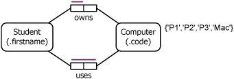
Map this onto a relational schema. Then populate the tables with these data:
Ann uses a P2.
Fred uses a P2 and a Mac, and owns a P2.
Sue uses a P3, and owns a PI.
Tom owns a Mac.
Given this schema and database, formulate the following queries in relational algebra and state the result. Make use of ∪, ∩, -, and [ ].
List the students who own or use a computer.
List the students who use a computer without owning one of that kind.
List the students who use a computer but own no computer.
List the students who own a computer but do not use a computer.
List the students who own a computer without using one of that kind.
List the students who use a computer and own a computer of that kind.
List the students who use a computer and own a computer.
List the computers used (by some student) but owned by no student.
List the computers owned (by some student) but used by no student.
If A is a 200 × 10 table and 5 is a 300 × 10 table, under what conditions (ifany) are the following defined?
(i) A ∪ B (ii) A ∩ B (iii) A – B (iv) A × B
(b) If A is 200 × 10 and B is 100 × 5, what is the size of A × B?
The relational schema and a sample population for a student database are shown here. Stu dents are identified by their student number. It is possible for two students to have the same name. All students have their name, degree, gender, and birth year recorded, and optionally subjects (e.g., a student might enroll in a degree before picking which subjects to study). Subjects are identified by their codes. Two subjects may have the same title. For each subject, we record the title and the credit. Some subjects might not be studied (e.g., PY205 might be a newly approved subject to be introduced in the next year). This schema applies to a one-semester period only, so we can ignore the possibility of student repeating a subject. Subject enrollments are entered early in the semester, and ratings are assigned at the end of semester (so rating is optional). Formulate each of the following queries as a single relational algebra query.
List the code, title, and credit for subject CS113.
List the student number, name, and degree of male students born after 1960.
List the codes of the subjects studied by the student(s) named “Brown T”.
List the studentNr and name of those students who obtain a 7 rating in at least one subject.
List the studentNr and name of all students who obtain a 5 in a subject called Logic.
List the studentNr and degree of those students who study all the subjects listed in the database.
List the studentNr, name, and gender of those students who either are enrolled in a BSc or have obtained a rating of 7 for PD102.
List the studentNr, name, and birth year for male students born before 1970 who obtained at least a 5 in a subject titled “Databases”.

The following table contains details on students who are to debate various religious topics. For this UoD, students are identified by their first name. Each debating team is to comprise exactly two members of the same religion but opposite gender.
Phrase each of the following as a single relational algebra query.
Debater: firstname gender religion Anne F Buddhist Betty F Christian Cathy F Hindu David M Christian Ernie M Buddhist Fred M Hindu Gina F Christian Harry M Buddhist Ian M Christian Jane F Christian Kim F Hindu List the name and religion of all females who are not Buddhist.
List the name and gender of those who are either male Hindus or female Christians.
List all possible debating teams, mentioning females before males. For example, one team comprises Anne and Ernie.
Map the following conceptual schema to a relational schema.

Use your schema to formulate each of the following in relational algebra.
Find names and salaries of all female employees who earn more than $25 000 or work on project “5GIS”.
List the name and gender of those employees who work on all projects with a budget of at least $100 000.
The Employee table stores the employee number and name of each employee, the department they work for, and the year they joined the firm. The Department table indicates the manager and budget for each department. Each employee manages at most one department (which must be the department for which he or she works).

Draw a conceptual schema diagram for this UoD.
Phrase each of the following requests as a single relational algebra query.
Who works for the Accounting department and started with the firm before 1970?
What is the budget of the department in which employee 133 works?
List the departmental managers and the year they joined the firm.
Which employees are not departmental managers?
Give the empNr, name, and year started for those managers of departments with a budget in excess of $50 000.
Which employees worked for the firm longer than their departmental managers?
Define A ∩ B in terms of –.
Let relation A have attributes x, y and relation B have attributes y, z where both y attributes are defined over the same domain. Define the natural inner join operation A ⋈ B in terms of ×, selection, and projection.
Let A have attributes x, y and B have the attribute y where both y attributes are defined over the same domain. Define A ÷ B in terms of ×, -, and projection.
In the following schema, a person is identified by the combining surname and forename. Formulate each of the following as single queries in relational algebra.

Which females play judo?
Which males in the weight range 70..80 kg play either judo or karatedo?
Which females over 50 kg play judo but not karatedo?
Who plays both judo and aikido? (Do not use a join.)
Who plays both judo and aikido? (Do use a join.)
The following relational schema relates to the software retailer UoD from Exercise 6.3. The category codes are: DB = Database; SS = Spreadsheet; WP = Word Processor.

Formulate the following as single queries in relational algebra.
List the customerNr of each customer who has been charged less than the list price for at least one software item, but has been sold no word processor.
List the name of each customer who was sold at least one copy of all the spreadsheets on the stock list.
List the customerNr of each customer who has purchased a copy of all the word processors that are in stock but who has never purchased a database.
List the customerNr of those customers who purchased both a spreadsheet and word processor on the same invoice.