12.6. SQL: Joins

We have seen how to choose, and order, columns and rows from a single table. But suppose the information we need from a single query is spread over many tables. SQL provides two main methods to access such information. The first of these uses relational joins and is discussed in this section. The second involves subqueries and is treated in a later section. The following discussion assumes a basic familiarity with the concept of joins from the relational algebra section.

A cross join (Cartesian product) of tables pairs all the rows of one with all the rows of the other. In SQL-89, a cross join of tables is specified by listing the tables in the from clause, using a comma”,” to denote the Cartesian product operator (depicted by “×” in relational algebra). A conditional join (⊖-join) selects only those rows from the Cartesian product that satisfy a specified condition. In SQL-89, the condition is specified in a where clause, just as we did in relational algebra. So the query expressions in Table 12.7 are equivalent.

Table 12.7. SQL-89 syntax for joins.

Join type	Relational algebra	SQL-89
Cross join	A × B	select * from A, B
Conditional join	A × Bwhere A.a ⊖ B.b	select * from A, B where A.a ⊖ B.b

Although the SQL-89 syntax has the advantage of being supported by every commercial dialect of SQL, it has drawbacks. First, it fails to distinguish join conditions (intertable comparisons) from nonjoin conditions (intratable comparisons on the same base row), instead lumping them together in a single where clause. This makes the query harder to understand. Second, it uses a comma for the cross join operation. This is unintuitive and also overloads the comma with different meanings (e.g., it is also used in SQL simply to separate items in lists). Third, it does not provide any direct support for operations such as outer joins, which can occur in practical queries.

For such reasons, SQL-92 (and later) uses special syntax for various kinds of join. In addition to supporting the SQL-89 syntax, these newer standards include special notations for the following types of join (any text after two hyphens “--” is a comment):

cross join qualified join:
	conditional join column-list join	-- on clause -- using clause
natural join union join

Qualified and natural joins may be further classified into the following types:

inner		-- this is the default
outer:	left right full

The new and old syntax for these is summarized in Table 12.8. In this summary, if tables A and B have any common columns (with the same local name), these columns are collectively referred to as “c”. For the column-list join, “c₁,...” denotes one or more of these common columns. Some entries for SQL-89 syntax include unions and sub-queries and are explained in later sections.

Table 12.8. Joins in SQL-92 onward, compared with SQL-89.

Join type	New syntax from SQL-92 onward	SQL-89 syntax
cross	select * from A cross join B	select * from A, B
conditional	select * from A join B         on condition	select * from A, B where condition
column-list	select * from A join B                 using (c1,...) -- c1,... are unqualified	select A.c1,..., ...      --omitB.c1,... from A, B where A.c1 = B.c1 and... --join columns are qualified
natural inner	select* from A natural [inner] join B --join column in result is c	select A.c,...            --omit B.c from A, B where A.c = B.c -- join column in result is A.c
left outer	select * from A natural left [outer] join B --join cols are unqualified; --nulls generated for non-matches --to join on fewer cols use: A left [outer] join B using (c1,...) --to join cols with different names: A left [outer] join B         on condition	select A.c,... omit B.c from A, B where A.c = B.c union all select c,...,‘ ? ’,... from A where c not in (select c from B) -- for composite c, use exists with a -- correlated subquery. -- fewer or different cols cases -- are not shown here
right outer	select * from A natural right [outer] join B -- other cases: cf. left join	select B.c,...     --omit A.c ... -- rest as for left join, -- but swap A and B
full outer	select * from A natural full [outer] join B --other cases: cf. left join; --rarely used	union of left and right outer joins
union	select * from A union join B --rarely used	select A. cols,‘ ’,... --‘ ’ ∀B col from A union all select‘ ’,..., B.cols --‘ ’ ∀ A col from B

Many dialects of SQL now support the new syntax for cross joins and qualified joins (including outer joins), but few yet support the new syntax for natural joins. Let’s now consider each of the new join notations.

For cross join, the more descriptive cross join may be used instead of a comma. This syntax is best reserved for unrestricted joins (full Cartesian products). As an example, Figure 12.41 shows details of Male and Female tennis players. The query lists possible male-female pairs for mixed-doubles teams. Cross joins are fairly rare in practice.

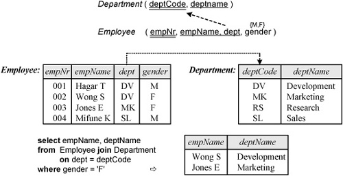
Much more common are conditional joins. The new syntax includes the join operator in the from clause, and the join condition in an on clause. Figure 12.42 shows a relational schema, a sample population, and a conditional join query to retrieve the name of each female employee and their department. To aid readability, it’s a good idea to indent the on clause, as shown. Each column mentioned in the query occurs in just one of the tables, so there is no need to qualify column names with table names. In this case, the join takes place along the foreign key reference shown in Figure 12.42. Although joins often involve foreign key references, they don’t have to. All we need is that the columns being joined are based on the same domain.

The same query may be formulated in SQL-89 as follows:

select empName, deptName

from Employee, Department

where dept = deptCode and gender = ‘F’

However, the formulation in Figure 12.42 is better, since it separates out the join condition (in the on clause) from the intratable condition (in the where clause). Although declaring the join conditions up front is logically cleaner, in practice, SQL optimizers typically evaluate the intratable conditions before the join conditions, since this reduces the size of intermediate tables created to compute the result (why?).

Column-list joins match values in the specified columns with the local same name in both tables. The new syntax uses the word join in the from clause, with the relevant columns listed in a using clause. As an example, consider the following schema. This is semantically equivalent to the previous schema, but different choices are made for some column names. The department code is denoted by “deptCode” in both tables, and the local identifier “name” is used for the department name, as well as the employee name.

Now consider the previous query: list the name of each female as well as their department name. How do we formulate this query for this new schema? The tables have two local column names in common: “deptCode” and “name”. Here we want to perform an equi-join between only some of the columns with common names (just “dept-code”, not “name”). The common column names used for the join are listed in a using clause, as shown here. Only one column is used for the join. To disambiguate the query, the column names in the select list are qualified by their table name.

select Employee.name, Department.name
from Employee join Department
    using (deptCode)
where gender = ‘F’

As you may have realized, the column naming choices in the previous two schemas are less than ideal. If two columns in different tables are intended to signify the same thing, it is better to give the columns the same name in those tables, wherever possible. Although informal, this makes it easier to see intended semantic connections between the tables, especially those without foreign key references. For the schema under discussion, “deptCode” may be uniformly used for the department code, and the names of employees and departments may be distinguished as “empName” and “deptName”, as follows:

With this new schema, the conditional join query considered earlier needs to qualify the column names used in the join, since their unqualified names occur in both tables. This gives

select empName, deptName
from Employee join Department
   on Employee.deptCode = DepartmentdeptCode
where gender = ‘F’

For the new schema, the column-list query does not require any qualifications to the column names, as shown here.

select empName, deptName
from Employee join Department
   using (deptCode)
where gender = ‘F’

As you might have noticed, the underlying join operation in the previous two queries is now a natural join, since we are equijoining on all the columns with the same name (in this case there is only one such column: deptCode).

As discussed in relational algebra, natural inner joins perform an equijoin to match all columns with the same local names and then remove the extra copies of these columns. In SQL-89, natural inner joins are specified by first forming the Cartesian product (of the tables listed in the from clause) and then specifying any join conditions in a where clause, using the select list to filter out unwanted duplicate columns. In SQL-92 (and later), natural inner joins may be declared simply by inserting natural or natural inner before join in the from clause (qualified and natural joins are inner by default).

The new notation has three main advantages: it is more descriptive; the natural join operator gives direct support for the natural inner join operator of relational algebra (⋈); and it is often more concise. For example, the query just considered can be reformulated more concisely as

select empName, deptName
from Employee natural join Department
where gender = ‘F’

There is no need to explicitly declare the join condition Employee.deptCode = DepartmentdeptCode, since this is implied by the use of natural and the fact that “deptCode” is the only common column name for the tables listed in the from clause. The compactness of this new notation is more obvious as the number of natural joins in a query grows. For example, consider the following relational schema.

Suppose we want to list the employee number and name of each employee who drives, as well as the model of their cars. Looking at the schema, the information is spread over three tables. As indicated in Figure 12.43, we can join the Employee and Drives tables by matching empNr, and join with the Car table by matching carRegNr (join values are shown in bold). Using the special syntax for natural joins, this can be formulated simply as shown.

Currently, most SQL dialects (including SQL Server) do not support the natural join syntax. Instead, the conditional join syntax is often used to handle natural joins. For example, the query in Figure 12.43 may be reformulated, thus:

select Employee.empNr, empName, carModel
from Employee join Drives
   on Employee.empNr = Drives.empNr
join Car
   on Drives.carRegNr = Car.carRegNr

Alternatively, SQL-89 syntax can be used as follows:

select Employee.empNr, empName, carModel
from Employee, Drives, Car
where Employee.empNr = Drives.empNr
  and Drives.carRegNr = Car.carRegNr

When the natural join operator is used, any join columns in the select list must be denoted by their local (unqualified) names. If a natural join is specified using other syntax (e.g., conditional join or SQL-89 syntax), the join columns must be qualified.

Although most joins in practice are natural inner joins, sometimes natural joins should be avoided. The natural join operation cannot be used to join columns with different names. For example, it can’t join dept and deptCode in the query of Figure 12.42. Moreover, the natural join operation must not be used if different tables in the from clause include columns with the same name that should not be equated. For example, consider the table schemes for our column-list join example: Department ( deptCode, name ); Employee ( empNr, name, deptCode, gender). A natural join between Department and Employee would equate not just deptCode but name as well. Any row in the result would equate the employee’s name with the department’s name, which is nonsense.

Sometimes we do wish to naturally join two tables on more than one column. For example, recall the following schema discussed in the relational algebra section.

To list the balance and client details for all the accounts requires a composite join on account (compound identifier) and a simple join on client. This may be specified with the natural join syntax as:

select * from Account natural join AcUser natural join Client

or as a conditional join:

select Account.branchNr, AccountaccountNr, balance,
Client.clientNr, clientName
from Account join AcUser
  on Account.branchNr = AcUser.branchNr
     and AccountaccountNr = AcUser.accountNr
   join Client
   on AcUser.clientNr = Client.clientNr

For conditional, column-list, and natural joins, join is assumed to mean inner join unless an outer join is explicitly specified (see later). In these cases, inner may be explicitly declared (e.g., inner join or natural inner join). If natural is declared, an on clause or a using clause must not be. If three or more tables are included in a join expression, the joins are normally evaluated in a left-to-right order. The join order can also be controlled by inserting parentheses. Since natural inner joins are associative, their order doesn’t affect the actual result.

As a more complex example, consider the relational schema in Figure 12.44. As an exercise, you might like to draw the conceptual schema. In the first table, “mgrEmpNr” denotes the employee number of the department manager (where there is a manager).

The pair-subset constraint indicates that an employee manages a department only if he or she works in it. The (2, 1) item-list marker on this constraint is used here to indicate the reordering of the pair of values to (mgrEmpNr, deptCode) before comparing with (empNr, deptCode).

Now consider the following query: for each department with a manager, list its code and name, and the employee number and name of its manager. We must match employee numbers between Department and Employee tables. The department codes must also match, but do we need to specify this? No, because if the manager referenced in the department table is the same as the employee referenced in the Employee table, the matching of department codes is implied by the constraints in the schema (why?). So the query may be formulated with the following conditional join:

select DepartmentdeptCode, deptName, mgrEmpNr, empName
from Department join Employee
  on mgrEmpNr = empNr

Can we do this with a natural join? No, since the join columns have different names (“mgrEmpNr” and “empNr”).

So far we have discussed four of the eight joins listed in Table 12.8. There are also three outer joins, as well as a union join. The union join is rarely used and is not discussed further. Outer joins may be left, right, or full. Left and right outer joins are often encountered in commercial applications. Given two tables A and B, their left/right/full outer join is formed by first computing their inner join and then adding the rows from the left/right/both table(s) that don’t have a match in the inner join and padding them with nulls to fill the extra columns in the result table.

Figure 12.45 provides a simple example of a natural left outer join. The query lists the employee number, name, and car registration numbers (if any) of all the employees (including those who don’t drive cars). Each of the two formulations shown is legal in SQL-92 (and later). The first uses the natural join syntax, but this is not yet supported by most SQL dialects. The second formulation uses the conditional outer join syntax, which is typically supported.

The natural inner join results in the three rows shown for the two drivers (employees 001 and 003). Employees 002 and 004 have no match in the Drives table. The left outer join adds their rows padded with a null value for car registration number. In this book, a null value is displayed as “?”. Some systems display it instead as a blank or as “NULL”. Many systems allow you to choose how you would like nulls to display.

Although the conditional join syntax requires qualified column names for join columns, when the result table is displayed, some systems (e.g., SQL Server) are clever enough to omit the table qualification from the column header (as in Figure 12.45). Some systems support an alternative outer join syntax that was introduced before outer joins became part of the SQL-92 standard. This alternative syntax often has different semantics and should never be used unless the standard syntax is unsupported.

SQL-92 (and later) are orthogonal. Anywhere that a value is legal, so is any expression that returns that value. This makes the language much easier to use and increases the expressive power of single queries. However, many commercial systems are not fully orthogonal. In particular, they often place restrictions on outer join queries. For example, at most one outer join might be allowed, or no other joins might be allowed after an outer join. With such systems, it is sometimes necessary to formulate a single standard query as a series of queries using intermediate tables to store results on the way.

Right outer join is analogous to left. Full join is the union of left and right. The word outer is assumed for left/right/full joins, so may be omitted (e.g., natural left join or left join). Outer joins are not associative, so be careful with the join order when outer joining three or more tables. As discussed later, outer joins can be emulated in the old SQL-89 syntax by means of union and subqueries.

When different rows of the same table must be compared, we need to join the table to itself. Such self-joins were discussed in Section 12.1. Recall that this requires introducing an alias for the table. In SQL, a temporary alias may be declared as a tuple variable in the from clause after the table it aliases. This variable may be assigned any row from the table and is sometimes called a “correlation variable”, “range variable”, or “table label”. For clarity, as may be used to introduce the alias.

Figure 12.46 provides a simple example. The base table Scientist stores the name and gender of various scientists, and the query lists pairs of scientists of opposite gender. Here the aliases SI and S2 are declared in the from clause. To understand the self-join, it helps to think of SI and S2 as copies of the original base table, as shown. The conditional join performs a <>-join on gender (to ensure opposite gender) and a <-join on PersonName (to ensure that each pair appears only once, rather than in both orders).

Some versions of SQL also provide a “create synonym” command for declaring a permanent alias definition. However, this is not part of the standard. In simplified form, the from clause syntax of SQL queries may be summarized in BNF as follows (for alternatives in braces, exactly one is required):

from table [ [as ] alias ]
   [, | cross join table [ [ as ] alias ]
      | natural [ inner | [ outer] {left | right | full} ] join table [ [as] alias ]
          | [ inner | [ outer ] {left | right | full} ] join table [ [ as] alias ]
                          { on condition | using (col-list)}
          | union join table [ [ as ] alias ]
          [,...]]

In formulating an SQL query, the guidelines discussed in relational algebra usually apply. First state the query clearly in English. Then try to solve the query yourself, watching how you do this. Then formalize your steps in SQL. This usually entails the following moves. What tables hold the required information? Name these in the from clause. What columns do you want, and in what order? Name these (qualified if needed) in the select list. If the select list doesn’t include a key, and you wish to avoid duplicate rows, use the distinct option. If you need n tables, specify the n -1 join conditions. What rows do you want? Specify the search condition in a where clause. What order do you want for the rows? Use an order by clause for this.

The new join syntax introduced in SQL-92 is convenient, but adds little in the way of functionality. The most useful notations are those for conditional and natural joins (both inner and outer). If you are using a version of SQL that does not support the new syntax, you should take extra care to specify the join conditions in detail and to qualify column names when required.

Any SQL statement may include comments. These might be used for explanation, documentation, or to simply comment out some code for debugging (comments are ignored at execution time). In SQL-92, a comment begins with two contiguous hyphens “--” and terminates at the end of the line. In addition to these single-line comments, SQL: 1999 introduced multiline comments, starting with “/*” and ending with “*/”. SQL Server supports both these comments styles. Here’s an example:

-- This query retrieves details about the employees who drive a car
select *     -- select all the columns
from Employee natural join Drives
/* If the natural join syntax is not supported,
       then omit “natural”, and specify the join condition in an on-clause */

Exercise 12.6