
11.3. Relational Mapping Procedure
The previous section introduced a generic notation for setting out a relational schema, and discussed simple examples of mapping from a conceptual to a relational schema. We now discuss the main steps of a general procedure for performing such a mapping. Advanced aspects of this procedure are considered in Section 11.4.
For a given conceptual schema, several different relational designs might be chosen. Ideally the relational schema chosen should be correct, efficient, and clear. Correctness requires the relational schema to be equivalent to the conceptual schema (within the completeness allowed by relational structures). Efficiency means good response times to updates and queries, with reasonable demands on storage space. Clarity entails that the schema should be relatively easy to understand and work with.
Since correctness of data is usually more important than fast response times, and correctness requires adequate constraint enforcement, a high priority is normally placed on simplifying the enforcement of constraints at update time. The main way to do this is to avoid redundancy. This strategy can lead to more tables in the design, which can slow down queries and updates if extra table joins are now required. For efficiency, we should try to keep the number of tables down to an acceptable limit.
With these criteria in mind, the Rmap (Relational mapping) procedure guarantees a redundancy-free relational design and includes strategies to restrict the number of tables. Rmap extends and refines an older mapping procedure known as the “Optimal Normal Form” (ONF) algorithm. The full version of Rmap includes details for completely mapping all graphical conceptual constraints and is beyond the scope of this book. However, the central steps of this procedure are covered in this section and the next.
As discussed in Chapter 14, more efficient relational designs with fewer tables may possibly result if the conceptual schema is transformed by an optimization algorithm before Rmap is applied, and sometimes lower level optimization using controlled redundancy may be needed to meet critical performance requirements.
Even without such further optimization, the Rmap procedure is extremely valuable since it guarantees a safe, reasonably efficient, normalized design. Happily, the basic steps of the procedure are simple. Redundancy is repetition of an atomic fact.
An atomic fact is typically elementary (e.g., The Scientist named ‘Einstein’ was born in the Country named ‘Germany’) but in rare cases could be existential (e.g. There exists a Country named ‘Germany’).
Having gone to the trouble of ensuring that our conceptual fact types are atomic, we can easily avoid redundancy in our relational tables.
Typically each row of a relational table stores one or more elementary facts. Otherwise the table row stores a single reference or existential fact (e.g., a lookup table of country names). Hence we can automatically avoid redundancy in tables by ensuring that each fact type maps to only one table in such a way that its instances appear only once.
To achieve this, there are two basic rules, as follows. As an exercise, convince yourself that grouping facts like this makes it impossible for any fact to be duplicated.
Each fact type with a compound, internal uniqueness constraint maps to a separate table by itself, keyed on the uniqueness constraint.
Fact types with functional roles attached to the same object type are grouped into the same table, keyed on the object type’s identifier.
These two rules show how to group fact types into table schemes. The first rule is illustrated in Figure 11.7. Any nonobjectified predicate with a uniqueness constraint spanning two or more of its roles must map to a table all by itself. Hence m:n binaries, and all n-aries (n ≥ 3) on the conceptual schema, map to a separate table (unless they are objectified associations, as discussed later).
Figure 11.7. Each fact type with a compound, internal UC maps to a table by itself.

Each object type maps to one or more attributes depending on the number of components in its reference scheme. If the predicate has only one uniqueness constraint, the table’s primary key is the attribute (or attribute set) spanned by this constraint. Otherwise one of the uniqueness constraints spans the primary key, and the others span alternate keys. ORM tools allow you to specify which constraint you prefer for the primary key before mapping.
When mapping conceptual schemas, care should be taken to choose meaningful table and column names. In the case of Figure 11.7, the table is used to store instances of the conceptual relationship type, so is often given a name similar to the conceptual predicate reading. If the object types involved are different, their names or the names of their value types, or a concatenation of the object and value type names, are often used as column names. For instance: Drives (empNr, CarRegNr).
When information about the same object is spread over more than one table, it is usually better to consistently use the same column name for this object, unless this loses an important distinction between the semantics of the different roles involved (e.g., empNr was also used in the Employee table to refer to employees). Apart from helping the designer see the connection, this practice can simplify the formulation of natural joins in the SQL standard. However, if different roles of the same predicate are played by the same object type, different column names must be chosen to reflect the different roles involved. For example: Contains(superpart, subpart, quantity).
A typical example of the second grouping rule is illustrated in Figure 11.8. Recall that a functional role has a simple uniqueness constraint. Here two functional roles are attached to the object type A. The rule also applies when there is just one functional role, or more than two. The handling of mandatory and optional roles was considered earlier (optional column in square brackets). The identification schemes of A, B, and C are not shown here, but may be simple or composite. The fact types are grouped together into a single table, with the identifier of A as the primary key (shown here as a).
Figure 11.8. Functional fact types of the same object type are grouped together.

The name of A is often chosen as the table name. To avoid confusion, it is best never to use the same name for both a table and a column, so the name of A’s value type is often chosen for a. The names of B and C (or their value types or role names) are often chosen as the other column names (here b and c). For example: Employee ( empNr, gender, [phone], salary, [tax]).
Once table groupings have been determined, keys underlined, optional columns marked in square brackets, and other constraints (e.g., subset, value list) mapped down, any derivation rules are also mapped, as discussed in the previous section.
To help understand the Rmap procedure it will help to consider several examples. In our initial examples, all entity types have simple identifiers, and no subtypes or objectified associations occur.
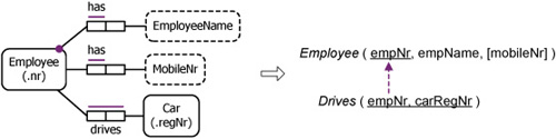
Consider the conceptual schema in Figure 11.9. The many:many fact type maps to a separate table (using rule 1), while the functional fact types map to a table keyed on the identifier of Employee (using rule 2). The primary keys are underlined, and the optionality of mobileNr is shown by the square brackets. The dotted arrow depicts the subset constraint that each employee referenced in the Drives table is also referenced in the primary key of the Employee table (referential integrity).
Figure 11.9. A simple relational mapping.
Now consider the ORM schema in Figure 11.10. Notice the equality constraint, shown as an arrow-tipped dotted line between the empNr fields of both tables. This is needed since both roles played by Academic are mandatory, and each maps to a different table. An equality constraint is equivalent to two subset constraints, going in opposite directions. This causes a referential cycle, since each table refers to the other.
Figure 11.10. The equality constraint entails a referential cycle.

The subset constraint from Qualification.empNr to Academic.empNr is a simple foreign key constraint, since it references a primary key. But the subset constraint from Academic.empNr to Qualification.empNr is not a foreign key constraint, since it targets only part of a primary key.
This latter subset constraint may be enforced in various ways (e.g., by assertions, triggers, or stored procedures). Referential cycles typically result from a role that has a mandatory constraint but no simple uniqueness constraint. Since referential cycles require special care to implement, this conceptual constraint pattern should be avoided if possible. In our example, however, the business rule that each academic holds at least one degree does seem reasonable, so in this case we leave it as is.
Before leaving this example, a few more comments about naming are worth making. The table name “Qualification” is one of many possible choices to convey the notion of academics being qualified by their degrees. Two other choices are to use the association name (“Holds”) or to concatenate the object type names (“AcademicDe-gree”). The department column is named “deptCode” because we expect other departmental facts (not shown here) to be recorded in a department table, and we want to avoid using “department” to name both a column and a table. Similarly, the degree column is named “degreeCode” rather than “degree”, since we might want to record other facts about degrees (e.g., their titles). In general, if the object type underlying a column will also underlie the primary key of another table, it is advisable to include the reference scheme in the column name.
Now consider Figure 11.11. Here each horse has its gender and weight recorded. Each race has at most one winner (we do not allow ties). There are no composite keys for rule 1 to work on. The gender and weight fact types have functional roles attached to Horse. By rule 2, these two associations must be grouped into the same table keyed on the identifier for Horse. Similarly, the time and win fact types are functions of race and are grouped into the Race table. We chose the column name “raceTime” instead of “time” mainly because “time” is a reserved word in SQL. It’s best to avoid using reserved words for names, since they require double quotes. We later provide links to online lists of SQL reserved words. The column name “winner” is used instead of “horseName” to convey the semantics better.
Figure 11.11. An ORM schema for horse races and its relational map.

Mapping 1:1 Associations
Let’s now consider some examples involving 1:1 fact types. In the conceptual schema of Figure 11.12, both Bankcard and Client share a 1:1 association. If we are certain that no other functional roles will be played by Bankcard, it is usually best to group the 1:1 fact type together with the other functional fact types into the same table, as shown.
Figure 11.12. The mapping choice if Bankcard plays no other functional roles.
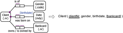
The bankcard column is optional, but the disadvantage of nulls here is usually outweighed by the advantage of having all the data in one table. The underlining of bank-card indicates a uniqueness constraint for its nonnull values. Because it may contain more than one null, the bankcard column cannot be used to identify rows, and hence cannot be the primary key. With two uniqueness constraints, we doubly underline clientNr to highlight it as the primary key.
If Bankcard does play other functional roles, however, the bankcard ownership association should be grouped into a Bankcard table, as shown in Figure 11.13. Notice that the owned role played by Bankcard is now explicitly mandatory; in the previous example it was only implicitly mandatory (because it was the only role played by Bankcard). Notice that only one role of this 1:1 association is mandatory. In asymmetric cases like this, it is usually better to group on the mandatory role side as shown.
Figure 11.13. The mapping choice if Bankcard plays another functional role.

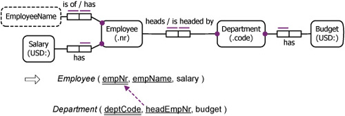
To illustrate this idea further, consider the conceptual schema in Figure 11.14. Here each employee is identified primarily by his/her employee number, but also has a unique name (unusual, but some departments work that way by refining formerly duplicate names). Each department has one head, who heads only one department. Since not all employees are department heads, the role of heading is optional. So the 1:1 association between Employee and Department is optional for Employee but mandatory for Department. Since it is usually better to group on the mandatory role side, here this means including the headEmpNr column in the Department table, as shown.
Figure 11.14. The heads fact type is grouped on the mandatory role side.
Suppose we grouped on the optional side instead, by adding a deptHeaded column to the Employee table. This leads to the following relational schema:

This alternative has two disadvantages. First, the optional deptHeaded column permits nulls (unlike the mandatory headEmpNr column). All other things being equal, nulls should be avoided if possible. In addition to consuming storage, they are often awkward for people to work with. The second disadvantage is that we now have an equality constraint between the tables, rather than just a subset constraint.
In principle, we might group into one table all the functional predicates of both object types involved in a 1:1 association. With our example this gives the scheme: EmployeeDept( empNr, empName, salary, [deptHeaded, deptBudget] ). Here enclosing the last two columns in the same square brackets declares that one is null if and only if the other is.
However, apart from requiring two optional columns and a special constraint that requires them to be null together, this grouping is unnatural. For example, the primary key suggests that the whole table deals with employees rather than their departments. For such reasons, this single-table approach should normally be avoided.
Now consider Figure 11.15(a). Here each employee has the use of exactly one company car, and each company car is allocated to exactly one employee. Employees and cars are identified by their employee number and by their registration number, respectively. The names of employees and the car models (e.g., Mazda MPV) are also recorded, but these need not be unique. Here both roles of the 1:1 association are mandatory, and each is attached to an entity type with another functional role. Should the 1:1 fact type be grouped into an Employee table or into a Car table?
Figure 11.15. The ORM schema (a) may map to relational schema (b) or to schema (c).
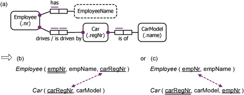
Unlike the previous example, we now have a symmetrical situation with respect to mandatory roles. An arbitrary decision could be made here. We could group to the left, as in Figure 11.15(b) or to the right as in Figure 11.15(c). Either of these approaches is reasonable.
We might also try a single table: EmployeeCar( empNr, empName, carRegNr, carModel). Although possible, it is unnatural, requiring an arbitrary choice of primary key. This becomes more awkward if other facts about employees (e.g., gender) and cars (e.g., purchase date) are recorded in the table. Also, consider the additional update overhead to change the car used by an employee, compared with the two table approach.
Now what about the case of a 1:1 fact type with both roles optional? For example, consider a UoD identical to that just discussed except that only some employees are given company cars and only some company cars are used by employees (e.g., some may be reserved for important visitors). The two table approach is recommended. Because of the symmetry with respect to mandatory roles, we could map the 1:1 association into the Employee table to give the schema: Employee( empNr, empName, [carRegNr]); Car( carRegNr, carModel); Employee.carRegNr references Car. Alternatively we could map it to the Car table yielding the schema: Employee( empNr, empName ); Car( carRegNr, carModel, [empNr]); Car.empNr references Employee. The percentage of nulls is likely to differ in these two designs. In this case, the design with fewer nulls is usually preferable.
Yet another option is a three table approach, in which the 1:1 association has a table to itself. This option becomes more attractive if the two table approach yields high percentages of nulls. For example, if only 1% of employees and 1% of cars are likely to be involved in Employee drives Car, we might map this fact type into a table by itself, giving three tables overall. A fourth option for 1:1 cases is to use two tables, but include the 1:1 association in both, with a special equality constraint to control the redundancy. More detailed discussions of mapping 1:1 fact types are referenced in the chapter notes. Our default procedure is summarized in Figure 11.16; here “functional role” means a functional role in an elementary fact type (not a reference type).
Figure 11.16. Default procedure for mapping 1:1 fact types.

In Figure 11.16, the arrow ![]() indicates that the 1:1 fact type should be grouped into the functional table of the left-hand object type. In case (a), the right-hand object type may play nonfunctional roles not shown here, and any role in the 1:1 fact type may be optional or mandatory. The third case (no other functional roles) is rare and requires a choice of primary key in the separate table. The final line refers to symmetric cases where the roles of the 1:1 predicate are both mandatory or both optional, and both object types play another functional role—here we have a grouping choice.
indicates that the 1:1 fact type should be grouped into the functional table of the left-hand object type. In case (a), the right-hand object type may play nonfunctional roles not shown here, and any role in the 1:1 fact type may be optional or mandatory. The third case (no other functional roles) is rare and requires a choice of primary key in the separate table. The final line refers to symmetric cases where the roles of the 1:1 predicate are both mandatory or both optional, and both object types play another functional role—here we have a grouping choice.
To understand some further cases, it will help to recall the fundamental bridge between conceptual and logical levels. This is summarized in Figure 11.17. In the populated ORM schema in Figure 11.17(a), the mandatory role pattern anticipates other roles being added later to Employee but not Gender. Figure 11.17(a) abbreviates the preferred reference schemes shown explicitly in Figure 11.17(b), which uses icons to directly depict a female employee and the female gender. The shaded, derived association abbreviates the conceptual path from EmployeeNr through Employee and Gender to GenderCode. This unpacks the semantics underlying the relational schema in Figure 11.17(c).
Figure 11.17. The conceptual/logical bridge.

Recall that uniqueness constraints on reference predicates are the responsibility of humans to enforce. The information system can’t stop us from giving the same employee number to two different employees, or giving the same employee two employee numbers. Hence uniqueness constraints on primary reference schemes are not mapped. Instead, we must enforce them in the real world.
Assuming that we have enforced the primary reference constraints however, the system can enforce constraints on the fact types. For example, it enforces the uniqueness constraint in Employee( empNr, gender) by ensuring that each employee number occurs only once in that column and hence is paired with at most one gender code. Assuming that the reference types really are 1:1, this uniqueness constraint on empNr corresponds to the uniqueness constraint on the conceptual fact type (i.e., Each Employee is of at most one Gender). It does not capture any uniqueness constraint from the reference types.
Mapping External Uniqueness Constraints
Let’s now consider mapping of schemas that include external uniqueness constraints. Recall that such constraints appear as a circled bar, and if they are used for preferred reference they have a double bar. In the ORM schema of Figure 11.18, employees are identified by combining their family name and initials. Since the external uniqueness constraint in this example underlies the preferred reference scheme, it is not mapped. In the resulting table scheme Employee( familyName, initials, gender ), the uniqueness constraint corresponds to the uniqueness constraint on the conceptual fact type Employee is of Gender. A good way to visualize the mapping is as follows:
Mentally erase the identification scheme of each object type.
Group facts into tables, using simple surrogates for the roles of real world objects.
Replace each surrogate by the attribute(s) used in the table to identify the objects.
Figure 11.18. Composite primary identifier, and functional fact type.

For example, the conceptual schemas of Figure 11.17 and Figure 11.18 each map initially to Employee( e, g) with the meaning Employee e is of Gender g. In both cases, g is then replaced by “gender”. With Figure 11.17, e is replaced by empNr, but with Figure 11.18, e is unpacked into family Name, initials since the identification scheme is composite. Since the uniqueness constraint spans e, it must also span the attribute combination that replaces it.
Now consider the conceptual schema of Figure 11.19. The structural difference here is that the fact type has a composite uniqueness constraint. We may initially think of it mapping to the table Drives( e,c). where e and c are surrogates for the employee and car roles. Replacing the surrogates by the real identifiers results in the table scheme Drives( familyName, initials, carReqNr). Since e was just part of a longer key, so is the composite identifier for employee that replaces it.
Figure 11.19. Composite primary identifier and nonfunctional fact type.

Now consider the conceptual schema of Figure 11.20. This is like that of Figure 11.18 except that Employee now has empNr as its primary identifier. The external uniqueness constraint now applies to two fact types rather than reference types, and hence can be mapped and enforced by the information system. As shown, this maps to a uniqueness constraint spanning surname and initials in the relational table (ensuring each familyName, initials combination is paired with only one employee number).
Figure 11.20. Composite secondary identifier and functional fact type.

The uniqueness constraint on the table’s primary key, empNr, captures the three simple uniqueness constraints on the three conceptual fact types (i.e., since each empNr is unique, it is paired with only one family name, only one sequence of initials, and only one gender).
Now consider the conceptual schema of Figure 11.21. Here each laboratory session is identified primarily by a session number and is used for a particular course. Once these course bookings have been made, sessions are assigned for use by students. The external uniqueness constraint says that each student is assigned at most one session for each course (e.g., laboratory resources might be scarce). Since this constraint involves fact types rather than reference types, it can be mapped.
Figure 11.21. External uniqueness constraint involving an m:n fact type.

An unusual feature of this example is the application of the external uniqueness constraint to a set of roles that includes a role in an m:n fact type (LabSession is assigned to Student).
Because the m:n fact type must map to a table by itself, the external uniqueness constraint spans two relational tables. This is equivalent to an internal uniqueness constraint spanning courseCode and studentNr in the natural join of the two tables.
Mapping Objectified Associations
Let’s now discuss some cases involving objectification (also known as nesting). In Figure 11.22 the association Employee worked on Project is objectified as Work. This objectified type plays one mandatory and one optional role, both of which are functional. As with other object types, we initially treat the objectified association as a “black box”, mentally erasing its identification scheme.
Figure 11.22. An active, objectified association with functional roles.

From this viewpoint, the conceptual schema appears to have just two fact types, both having functional roles attached to the object type Work. Fact types are now grouped in the usual way. So these two fact types are grouped into the same table. Visualizing the nested object type Work as a black box “▪” results in the table: Work(▪, startdate, [enddate]). Finally we unpack ▪ into its component attributes (empNr and projectName), giving Work( empNr, projectName, startdate, [enddate]).
The value constraint in Figure 11.22 verbalizes as: For each Work, existing enddate >= startdate. This may be alternatively specified as a textual constraint. As discussed in Section 7.4, value constraints are violated if and only if they evaluate to false (just like SQL check clauses). The footnote annotation on the relational schema here corresponds to the SQL check clause check (enddate >= startdate).
Independent object types, whether nested or not, require special treatment in mapping, as follows.
Map each independent object type and the fact types (if any) in which it plays functional roles to a separate table, with the object type’s identifier as the primary key, and all other attributes optional. Add a subset constraint to this primary key from each column sequence mapped from nonfunctional roles (if any) of the independent object type.
Consider the ORM schema of Figure 11.23. Here employees might be assigned to projects before their actual starting date is known. So some instances of the objectified Assignment association might be recorded that (in some database state) do not play either of the attached roles. In this example, since even the disjunction of the attached roles is optional, the nested object type is independent—this is noted by the exclamation mark in “Assignment !”. Contrast this with the previous example (Figure 11.22), where the nested object type Work is active.
Figure 11.23. Mapping an independent, objectified association with functional roles.

If we wish to record just the fact that an employee is assigned to a particular project, we enter values just for empNr and projectName. Details about start and end dates for work on the project can be added later when they are known. Since both start date and end date are optional, the value constraint now verbalizes as: For each Assignment, existing enddate >= existing startdate.
Figure 11.24 shows another way to model this UoD. Here the independent object type has no functional roles attached. In this case, it maps to a table all by itself. The m:n fact type maps to another table. A subset constraint captures its optionality. If instead we tried to map everything to one table, this would violate entity integrity (why?).
Figure 11.24. Mapping an independent, objectified association with no functional roles.

The constraint that if an assignment’s start and end dates are known, the end date must come after or on the start date is now harder to formulate, both at the conceptual level and at the relational level. Moreover, the approach of Figure 11.24 spreads the information over more tables and demands an intertable constraint. This is usually undesirable, since it often slows down the execution of queries and updates. For such reasons, the approach of Figure 11.23 is normally preferred to that of Figure 11.24.
Notice that the schemas in Figure 11.23 and Figure 11.24 allow us to record an end date without a start date. In practical applications, we sometimes allow things like this because our information may be incomplete. For example, we might want to record the date somebody ended a project, but not know when that person started. For the same reason, conceptual schemas sometimes have fewer mandatory roles than the ideal world suggests, and in consequence relational schemas may have more optional columns than complete knowledge would allow.
Suppose, however, that if we know an end date then we do know the starting date. To enforce this constraint in Figure 11.23, add a subset constraint on the ORM schema from the first role of the “ended on” predicate to the first role of the “started on” predicate. This constraint may be declared in the relational schema by using nested option brackets. Here we enclose the option brackets for enddate inside the option brackets for startdate, giving: Assignment( empNr, projectName, [ startdate, [enddate] ]). This indicates that a (nonnull) value is recorded for enddate only if a value is recorded for startdate.
To add this constraint to Figure 11.24 is not as easy. A textual constraint is required at both conceptual and relational levels to declare that for each employee, project pair, phase “end” is recorded only if phase “start” is.
Chapter 14 examines in detail the notion of “equivalent” conceptual schemas and provides guidelines for transforming a conceptual schema to improve the efficiency of the relational schema obtained from Rmap.
If the start and end dates for an employee’s work on a project are recorded, a derivation rule can be specified to compute the work period (by subtracting the start date from the end date, if known). Since each computer system has an internal clock, conceptually there is a unary fact type of the form: Date is today. So for someone still working on a project we could also derive the time spent so far on the project by subtracting the start date from the current value for “today”.
By default, derived facts are not stored. So by default, derived columns are excluded from the base tables (i.e., stored tables) of the relational schema. For example, the derivation rules could be implemented using views or stored procedures.
In some cases, efficiency considerations may lead us to derive on update rather than at query time, and store the derived information. In such cases the derived fact type is marked “**” on the conceptual schema diagram. During the relational mapping, the fact type is mapped to a base table, and the derivation rule is mapped to a rule that is triggered by updates to the base table(s) referenced in the derivation rule. For example, we could implement the derivation rule by declaring appropriate generated columns or table triggers (recall the earlier net pay example). As well as derivation rules, all conceptual constraints should be mapped (not just uniqueness and mandatory constraints).
Mapping Subtypes
Let’s now consider the mapping of subtype constraints. Table 11.1 was met earlier in Chapter 6. Although we have no rule to determine when a phone number is recorded, we know that prostate status may be recorded only for male patients, and pregnancies are recorded for all female patients and only for female patients. The conceptual schema is reproduced in Figure 11.25.
| PatientNr | Name | Gender | Phone | Prostate status | Pregnancies |
|---|---|---|---|---|---|
| 101 | Adams A | M | 2052061 | OK | – |
| 102 | Blossom F | F | 3652999 | – | 5 |
| 103 | Jones E | F | ? | – | 0 |
| 104 | King P | M | ? | benign enlargement | – |
| 105 | Smith J | M | 2057654 | ? | – |
Figure 11.25. Subtype constraints on functional roles map to qualified optionals.

Some limited support for subtyping is included in the SQL standard, but current relational systems typically do not support this concept directly. Nevertheless, there are three main ways in which subtyping can be implemented on current systems: absorption, separation, and partition. With absorption, we absorb the subtypes back into the (top) supertype (giving qualified optional roles), group the fact types as usual, and then add the subtyping constraints as textual qualifications, as shown in Figure 11.25.
To best understand this example, visualize the subtypes on the conceptual schema being absorbed back into the supertype Patient, with the subtype roles now attached as qualified optional roles to Patient. All the roles attached to Patient are functional, so the fact types all map to the same table, as shown. The phone, prostateStatus, and nrPregnancies attributes are all optional, but the latter two are qualified.
In the qualifications, “exists” means the value is not null. Qualification 1 is a pure subtyping constraint, indicating that a nonnull value for prostate status is recorded on a row only if the value of gender on that row is ‘M’. Some men might have a null recorded here. Qualification 2 expresses both a subtype constraint (number of pregnancies is recorded only if gender is ‘F’) and a mandatory role constraint (nrPregnancies is recorded if gender is ‘F’). Recall that “iff” is short for “if and only if”.
Since only functional fact types are involved in this example, the absorption approach leads to a table that basically matches that of the original output report (except that most relational systems support only one kind of null). The main advantage of this approach is that it maps all the functional predicates of a subtype family into a single table. This usually makes related queries and updates more efficient. Its main disadvantage is that it generates nulls.
The second main approach, separation, creates separate tables for facts with subtype specific functional roles. With this approach, the conceptual schema of Figure 11.25 maps to three tables: one for common facts, one for male-specific facts, and one for female-specific facts.
The third main approach, partition, may be used when the subtypes form a partition of their supertype. Since MalePatient and FemalePatient are exclusive and exhaustive, this approach may be used here, resulting in two tables: one containing all the facts about the male patients and the other all the facts about female patients.
The next section discusses the relative merits of these three approaches and also considers mapping cases where subtypes use a preferred identification scheme different from the supertype’s. Our default approach, however, is to absorb the subtypes before grouping. Note that even with this approach, any fact types with a nonfunctional role played by a subtype map to separate tables, with their subtype definitions expressed by qualified subset constraints targeting the main supertype table.
For example, the ORM schema in Figure 11.26 adds the optional m:n fact type to FemalePatient: FemalePatient attended prenatal clinic on Date. This fact type maps to a separate table with the qualified subset constraint “only where gender = ‘F’”, as shown. If the new fact type were instead mandatory for FemalePatient, the qualification would read “exactly where” instead of “only where”.
Figure 11.26. Nonfunctional fact type of subtypes map to separate tables.

We have now covered all the basic steps in the Rmap procedure. These are now summarized. Even if you are using a CASE tool to do the mapping for you, it’s nice to understand how the mapping works.
| 0 | Absorb subtypes into their top supertype. Mentally erase all explicit preferred identification schemes, treating compositely identified object types as “black boxes”. |
| 1 | Map each fact type with a compound UC |
| 2 | Fact types with functional roles attached to the same object type |
| 3 | Map each independent object type with no functional roles to a separate table. |
| 4 | Unpack each “black box column” into its component attributes. |
| 5 | Map all other constraints and derivation rules.Subtype constraints on functional roles map to qualified optional columns, and those on nonfunctional roles map to qualified subset constraints. Nonfunctional roles of independent object types map to column sequences that reference the independent table. |
Step 0 may be thought of as a preparatory mental exercise. Erasing all explicit preferred reference schemes (i.e., those shown other than by parenthesized reference modes) ensures that all the remaining predicates on display (as box sequences) belong to fact types (rather than reference types). Recall that a compositely identified object type is either a nested object type (objectified association) or a coreferenced object type (identified via an external uniqueness constraint).
There are plenty of questions in the section exercise to give you practice at performing the mapping manually. As preparation for this exercise, some larger examples are now considered. Figure 11.27 shows the conceptual schema for the compact disc case study discussed in Chapter 5. If you feel confident, you might like to try mapping this to a relational schema yourself before reading on.
Figure 11.27. The conceptual schema from the compact disc case study.

As there are no subtypes in this example, step 0 amounts to mentally erasing any preferred reference schemes that are shown explicitly. There are only two, each involving a compositely identified object type: Track and Listing. Figure 11.28 depicts this erasure by removing the predicate boxes and showing their connections to object types as dashed lines. For steps 1 – 3 we treat these two, compositely identified entity types just like any other entity type.
Figure 11.28. The reference types are erased, and fact types are lassoed into groups.
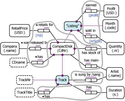
We now proceed to group fact types into tables. To help visualize this we place a lasso around each group of predicates that map to the same table (see Figure 11.28). We lasso only the predicates, not the object types. Since each fact type should map to exactly one table, all predicates must be lassoed, and no lassos may overlap.
In step 1 we look around for a predicate with a compound uniqueness constraint. Since the objectified association is now hidden, we see only one such predicate: is sung by. So we lasso this predicate, indicating it goes to a table all by itself.
In step 2 we group functional fact types of the same object type together. For example, CompactDisc has five functional roles attached to it, so these five fact types are grouped into a table keyed on the identifier for CompactDisc. Similarly the two functional fact types for Track are lassoed together, as are the two functional fact types of the nested object type.
This example has no 1:1 cases, and no independent object types. We have now roped all the predicates, and there are four lassos, so the conceptual schema maps to four tables.
The final relational schema is shown in Figure 11.29. Since five functional fact types map to the CD (CompactDisc) table, and all the objects involved have simple identifiers, this table has six columns (one for the key and one for each fact attribute). The other three tables involve a compositely identified object type, which is unpacked into its component attributes (step 4).
Figure 11.29. Relational schema mapped from the conceptual schema in Figure 11.27.

The keys of the tables are already determined, but the mandatory role constraints are enforced by mandatory columns and inter-table subset/equality constraints. Note the composite subset constraint from the pair cdNr, trackNr in Vocals to the primary key of Track. Finally the two derivation rules are mapped (step 5).
If you lasso fact types into groups before writing down the table schemes, you may mentally erase all preferred identification schemes (including reference modes) in step 0 (thus treating all object types as black boxes) and then in step 4 replace each column by its identifying attribute(s). This alternative formulation of the Rmap procedure is logically cleaner. If performing Rmap manually, you might find it convenient to photocopy the conceptual schema and use colored pencils to cross out the reference types and lasso the fact types.
As a complicated example, consider the ORM schema in Figure 11.30. This concerns television channels. Notice that TimeSlot is modeled as a coreferenced entity type (a time slot is identified as a given hour on a given day). For variety, the object types Office and Department are modeled as objectified associations. A television channel may have different offices in different suburbs. For this UoD, a channel may have only one office in any given suburb. A given office may have many departments.
Figure 11.30. An ORM schema for TV channels.

For example, one department might be the advertising department for the channel 9 office located in the suburb Toowong. Alternatively (and arguably more naturally), the object types Office and Department could have been modeled as coreferenced object types. However this would not change the mapping.
The external uniqueness constraint on Program indicates that a channel can screen only one program at a given time. As an exercise, try to map this yourself before reading on. Start by mentally erasing the reference types and lassoing the fact types that should be grouped together before you write down the relational schema.
Figure 11.31 hides the identifying predicates for Time, Office and Department, and lassos the fact types into groups. The 1:1 associations must be grouped with Channel and Program since these have other functional roles, but Frequency and Title do not.
Figure 11.31. Reference types are erased, and fact types are grouped.

The detailed relational schema is shown in Figure 11.32. The identifier for Office unpacks into two attributes, while the Department key unpacks into three (two for Office and one for DepartmentKind). Notice also the intertable uniqueness constraint. This indicates that when a natural join is performed between the Program and Prog-Time tables, there will be a uniqueness constraint spanning the three columns chan-nelNr, progDay, and progHour. In other words, for any given channel and time, there is at most one program being shown.
Figure 11.32. A relational schema mapped from the model in Figure 11.30.

Notice the many equality constraints in the relational schema. These lead to referential cycles that may be awkward to implement. The many mandatory roles also entail that a lot of data must be entered in a single transaction. As discussed earlier, to minimize referential cycles, you should not add a mandatory role constraint to a nonfunctional role unless it is absolutely required.
As an optional exercise, you may wish to consider which mandatory role constraints would best be removed from Figure 11.30.
The following exercise contains many questions to give you practice with relational mapping. The choice of names for tables and columns is up to you, but you may wish to consider the naming guidelines discussed earlier.
Mapping from a conceptual to a relational schema is a bit like doing CSDP step 1 in reverse. Try to choose names for tables and columns that would make it easier for you to perform CSDP step 1 if presented with the relational tables. Remember that tables are basically just collections of facts.
Exercise 11.3
Map the following conceptual schema onto a relational schema using the Rmap procedure. Use descriptive table and column names. Underline the keys, and enclose any optional columns in square brackets. Indicate any subset or equality constraints.

Rmap the following conceptual schema.
The conceptual schema for a given UoD is shown. A novice designer maps the likes and costs fact types into a single table: Likes ( woman, dress, cost). With the aid of a small, sample population, explain why this table is badly designed. Use surrogates wl, w2, ... for women and dl, d2,... for dresses.
Rmap the conceptual schema.

In a given UoD, each lecturer has at least one degree and optionally has taught at one or more institutions. Each lecturer has exactly one identifying name, and at most one nickname. Each degree is standardly identified by its code, but also has a unique title. Some degrees might not be held by any lecturer. Each institution is identified by its name. The gender and birth year of the lecturers are recorded, as well as the years in which their degrees were awarded.
A novice designer develops a relational schema for this UoD that has the following two tables. Explain, with the aid of sample data, why these tables are badly designed.
Lecturer (lecturerName, gender, degreeCode, degreeTitle)
Qualification ( degreeCode, yearAwarded )
Draw a conceptual schema for this UoD.
Rmap your answer to (b).
Add constraints to your conceptual schema for the following and then perform Rmap.
Exercise 3.5, Question 2.
Exercise 3.5, Question 3.
Rmap the Invoice conceptual schema for Exercise 6.3, Question 3.
Rmap the Oz Bank conceptual schema for Exercise 6.4, Question 6.
Consider a naval UoD in which sailors are identified by a sailorNr, and ships by a shipNr, although both have names as well (not necessarily unique). We must record the sex, rank and birthdate of each sailor and the weight (in tonnes) and construction date of each ship. Each ship may have only one captain and vice versa. Specify a conceptual schema and relational schema for this UoD for the following cases.
Each captain commands a ship but some ships might not have captains.
Each ship has a captain but some captains might not command a ship.
Each captain commands a ship, and each ship has a captain.
Some captains might not command a ship, and some ships might not have captains.
Consider a UoD in which students enroll in subjects, and later obtain scores on one or more tests for each subject. Schematize this conceptually using nesting and then Rmap it.
Assume that scores are available for all enrollments.
Assume that enrollments are recorded before any scores become known.
Rmap the conceptual schema in Figure 6.46 (absorb the subtypes before mapping).
Refer to the MediaSurvey conceptual schema in Figure 6.53.
Rmap this schema (absorb subtypes).
Set out an alternative relational schema with separate tables for each node in the subtype graph. Which schema is preferable?
Rmap the Taxpayer conceptual schema for Exercise 6.5, Question 3(a).
Rmap the Taxpayer conceptual schema for Exercise 6.5, Question 3(b).
Rmap the SolarSystem conceptual schema for Exercise 6.5, Question 6.
Rmap the conceptual schema in Figure 7.5 (note that Panel is an independent object type).
Rmap the CountryBorders conceptual schema for Exercise 7.3, Question 5.
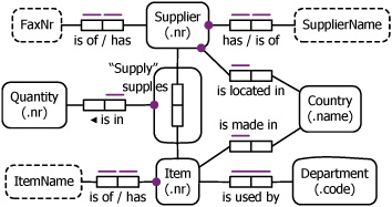
Rmap the IT Company schema shown.
Rmap the University schema shown. Note that Degree is compositely identified (e.g., a Ph.D. from UCLA and a Ph.D. from MIT are treated as different degrees). Student is also compositely identified (by the time you finish the mapping, you will appreciate how much better it would be to use a studentNr instead!). The codes ‘y’, ‘n’, ‘PT’, ‘FT’, ‘int’, and ‘ext’ abbreviate “yes”, “no”, “part time”, “full time”, “internal”, and “external”.
IT Company Schema

University Schema

Rmap the following conceptual schema. Ignore the implicit semantic connection between Year and Date.

A life insurance company maintains an information system about its clients. The following information samples are extracted from a fragment of this system. For simplicity, several data items (e.g., client’s name and address) are omitted and may be ignored for this question. Each client is identified by his/her client number (clientNr).
The following table uses these abbreviations: Emp. = employment (EA = Employed by Another; SE = Self-Employed; NE = Not Employed); Acct = accounting; NS = Non-Smoker; S = Smoker. Some clients are referred by other clients (referrers) to take out a policy (this entitles referrers to special benefits outside our UoD). The value “?” is an ordinary null value meaning “not recorded” (e.g., non-existent or unknown). The value “-” means “inapplicable” (because of some other data).
ClientNr Referrer Birth date Smoking status Emp. status Job Work phone Acct. firm 101 ? 15/2/46 NS EA lecturer 3650001 – 102 ? 15/2/46 S SE builder 9821234 Acme 103 101 1/1/70 NS NE – – – 104 103 3/4/65 S EA painter ? – 105 ? 1/1/70 NS SE painter 2692900 ? For each client a record of major illnesses (if any) is kept; one recovery figure and hospital is noted for each client illness. The extract for clients 101-105 is shown.
ClientNr Illness Degree (%) of recovery Hospital treated 102 stroke 90 Wandin Valley diabetes 80 Burrigan 103 diabetes 95 Wandin Valley Each client selects one insurance coverage (currently $25,000, $50,000, or $100,000) and pays a monthly premium for this coverage. Premiums are determined by coverage, age, and smoking status, as shown in the following schedule. This schedule is stored in the database (it is not computed by a formula). From time to time, this schedule may change in premiums charged, coverages offered, or even age groups. Premiums for both smokers and non-smokers are always included for each age group/coverage combination. For simplicity, only the latest version of the schedule is stored (a history of previous schedules is not kept). Moreover, payments must be for 1 year at a time and are calculated as 12 times the relevant premium current at the date of payment (using the age of the client at that date).
The computer system has an internal clock, which may be viewed conceptually as providing an always up-to-date instance of the fact type: Date is today. You may use “today” as an initialized date variable in derivation rules.

Although not shown in the schedule, age groups are identified primarily by an age group number (currently in the range 1..4). Assume that all clients have paid their 12-month fee by completing a form like that shown here (details such as name and address are omitted for this exercise). The first four fields are completed by the insurance agency and the rest by the client. Records of any previous payments are outside the UoD.

Choose suitable codes to abbreviate payment methods and card types. Each credit card is used by at most two clients (e.g., husband and wife). In practice the card type could be derived from the starting digits of the card number, but ignore this possibility for this question.
Specify a conceptual schema for this UoD. Include all graphic constraints and any noteworthy textual constraints. Include subtype definitions and derivation rules. If a derived fact type should be stored, include it on the diagram with an “**” mark to indicate it is both derived and stored.
Should the payment by a client be derived only, stored only, or both? Discuss the practical issues involved in making this decision.
Map your conceptual schema to a relational schema, absorbing subtypes while maintaining subtype constraints. Underline keys and mark optional columns with square brackets. Include all constraints. As an optional exercise, map any derivation rules.