14.6. Normalization

The process of mapping from a conceptual schema expressed in atomic fact types to a relational schema involving table types is one of deconceptualization. This approach facilitates sound design primarily because it emphasizes working from examples, using natural language, and thinking in terms of the real-world objects being modeled.

The advantages of using elementary facts are clear: working in simple units helps get each one correct; constraints are easier to express and check; nulls are avoided; redundancy control is facilitated; the schema is easier to modify (one fact type at a time); and the same conceptual schema may be mapped to different logical data models (so decisions about grouping fact types together may be delayed until mapping).

Nowadays, many database designers do a conceptual design first, whether it be in ORM, ER, or UML notation, and then apply a mapping procedure to it. In the past, in place of conceptual modeling, many relational database designers used a technique known as normalization. Some still use this, even if only to refine the logical design mapped from the conceptual one. If an ORM conceptual schema is correct, then the table design resulting from Rmap is already fully normalized, so ORM modelers don’t actually need to learn about normalization to get their designs correct. However, a brief look at normalization is worthwhile, partly to consolidate aspects of good design and partly to facilitate communication with those who use the normalization approach.

There are two techniques for normalization: synthesis and decomposition (sometimes called “analysis”). Each operates only at the relational level and begins with the complete set of relational attributes, as well as a set of dependencies on these, such as functional dependencies (FDs). Recall that if X and Y are simple or composite attributes (sets of one or more column headers), we say that X functionally determines Y (written X → Y) if and only if for each value of X there is at most one value of Y.

In any realistic business domain it is too easy to get an incorrect model if we begin by simply writing down a list of attributes and dependencies, since the advantages and safeguards of conceptual modeling are removed (e.g., validation by verbalization and population). Moreover, the set of dependencies considered in normalization is usually very limited, so that many UoD constraints are simply ignored.

The output of both synthesis and decomposition techniques is a set of table schemes each of which is guaranteed to be in a particular “normal form”. We will have a closer look at normal forms presently. The synthesis algorithm basically groups attributes into tables by finding a minimum, reduced, annular cover for the original dependencies. Redundant FDs (e.g., transitive FDs) are removed, redundant source attributes (those on the left of a “→”) are removed, and FDs with the same source attribute are placed in the same table. With respect to its specified class of dependencies and attributes, the synthesis algorithm guarantees a design with the minimum number of tables, where each table is in elementary key normal form (see later for a definition of this concept).

For example, given the FDs {empNr → gender, empNr → birthdate, empNr → job, job →> salary, empNr → salary}, synthesis generates two tables: R1(empNr. gender, birthdate, job ); R2{ job, salary). While this example is trivial, for more complex cases the execution of the synthesis algorithm is arduous and is best relegated to a computer. It should be apparent that the derived fact type checks in the CSDP, and the basic fact type grouping in Rmap, have a close correspondence to the synthesis method.

Although synthesis has often been taught in academia it is rarely used by practitioners, partly because of its highly technical nature, but mainly because it is almost useless in practice. The main problem with synthesis is that it assumes for its input a correct global set of attributes and dependencies. In practice, however, such an input is rarely available, and determining such an input is often harder than determining the correct design by other means. For such reasons, we essentially ignore the synthesis technique from this point on.

Another problem with normalization (by synthesis or decomposition) is that it can’t change the set of attributes. Hence, apart from ignoring transformations that involve other kinds of constraint, normalization misses semantic optimization opportunities that might arise by allowing transformations to change attributes.

For example, the FD set {department → budget, (department, gender) → nrStaff} synthesizes to two table schemes R1(department, budget) and R2(department, gender. nrStaff). But normalization is unable to transform the FD set into {department → budget, department → nrMaleStaff, department → nrFemaleStaff}, which would lead to the single table design R{department, budget, nrMaleStaff, nrFemaleStaff). Compare this with the ORM schema optimization approach just discussed.

Considerations such as these indicate that use of normalization alone is inadequate as a design method. Nevertheless the use of normalization as a check on our conceptual modeling may at times be helpful. On the positive side, by limiting their scope to a small but important class of constraints, and ignoring semantic transformations, normalization theorists have been able to establish several interesting results.

Unlike synthesis, the decomposition approach to normalization is an iterative one, progressively splitting badly designed tables into smaller ones until finally they are free of certain update anomalies, and it provides no guarantee of minimality of number of tables. However, the decomposition approach is more well known, and some modelers find its principles useful for correcting poor relational designs. The rest of this section focuses on the decomposition approach, with some comparisons to ORM. To assist the reader who may read this section out of sequence, some basic concepts treated earlier are reviewed briefly.

A relational schema obtained by Rmapping it from a correct ORM conceptual schema is already fully normalized. Suppose, however, that some error was made in either the conceptualization or the mapping, or that the relational schema was designed directly without using a conceptual schema. It is now possible that some of the table designs might be unsafe because some conceptual constraint is not enforced. If a conceptual constraint may be violated when a table is updated by inserting, deleting, or modifying a row, the table design is said to contain an update anomaly.

Constraints on conceptual reference types are the responsibility of humans. Only people can ensure that preferred reference schemes actually do provide a correct 1:1-into map from real-world entity sets to sets of data values (or data tuples). Special care is required when an entity type plays just one fact role, this role is not functional, and an instance of this entity type changes its preferred identifier.

For example, suppose City occurs only in the m:n fact type: RussianTour(.nr) visits City (.name). In the early 1990s, the city then known as “Leningrad” reverted to its original name “Saint Petersburg”. As an exercise, discuss some problems arising if only some instances of “Leningrad” are renamed.

Assuming preferred reference schemes are already enforced, the information system itself should normally enforce all the fact type constraints. So all constraints on (and between) conceptual fact types should be captured in the relational schema. The normalization procedure ensures that most of these constraints are so captured. In particular, it aims to remove any chance of redundancy (repetition of an elementary fact). If a fact were duplicated in the database, when the fact changed it would be necessary to update every instance of it, otherwise the database would become inconsistent.

Starting with a possibly bad table design, the normalization procedure applies rules to successively refine it into higher “normal forms” until it is fully normalized. Let’s confine our attention to the normal forms that focus on eliminating problems with a table by splitting it into smaller ones. There are many such normal forms. In increasing order of acceptability, the main ones are first normal form (1NF), second normal form (2NF), third normal form (3NF), elementary key normal form (EKNF), Boyce/Codd normal form (BCNF), fourth normal form (4NF), fifth normal form (5NF), and domain key normal form (DKNF). We’ll discuss each of these in turn.

A table that is not in first normal form is said to be “unnormalized” or in Non-First Normal Form (NFNF = NF²). A table in a higher normal form is also in its lower normal forms (e.g., a 3NF table is also in 2NF and 1NF). Hence tables may be classified as shown in Figure 14.56. A table’s highest normal form (hNF) is its deepest normalization level.

The first three normal forms were originally proposed by E. F. (“Ted”) Codd, who founded the relational model of data. The other forms were introduced later to cater for additional cases. These improvements were due to the work of several researchers, including E. F. Codd, R. Boyce, R. Fagin, A. Aho, C. Beeri, and J. Ullman. Other normal forms have also been proposed (e.g., horizontal normal form and nested normal form) but are not discussed here.

A table is normalized, or in first normal form (1NF), if and only if its attributes are single valued and fixed. In other words, a 1NF table has a fixed number of columns, and each entry in a row-column position is a simple value (possibly null). Almost every table we’ve seen so far in this book has been in INF.

A table may violate 1NF (and hence be an NF² table) either by having multivalued attributes (e.g., entries that are collection such as sets, arrays, or even relations) or by allowing different rows to have different numbers of attributes.

As an example of the first kind of violation, consider Table 14.7. While the first two columns in this Student table store only atomic values, the Car column stores sets of values, and the Result column holds sets of (course, rating) pairs.

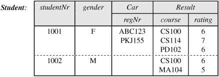
To model this in a relational database we need to flatten the structure out into three tables: Student (studentNr. gender); Drives( studentNr. car); and Scores( studentNr, course, rating). Hence, 1NF relations are often called flat relations.

However, it is possible to model the structure directly by using a relation that is not in first normal form. For example, we might use the following nested relation scheme:

Student, (studentNr, gender, Car regNr), Result course, rating))

Here an entry in the third column is itself a relation (in this case, a set of car registration numbers). Similarly, each entry in the Result column is a relation (with course and rating attributes). Since the logical data model underlying this approach allows relations to be nested inside relations, it is called the nested relational model.

Since the nested table is not in 1NF, it is not a relational table (i.e., it does not conform to the relational model of data). Although pure nested relational systems have yet to make any significant commercial impact, many of the major relational DBMSs have evolved into object-relational systems with support for NF² tables, as discussed in the next section. While tables not in 1NF might be in some other exotic “normal form”, it is common practice to refer to them as being “unnormalized”.

Set-valued fields such as Car in Table 14.7 are sometimes called “repeating attributes”, and fields such as Result that hold sets of grouped values are sometimes called “repeating groups”. This term may be used to include the notion of repeating attribute by allowing degenerate groups with one value. Using this older, if somewhat misleading, terminology we may say that 1NF tables have no repeating groups.

Another example of an unnormalized table is the “variant record type” used in languages such as Pascal and Modula. Here different “rows” in the same record type may contain different fields. For example, the Figure record type in Figure 14.57 is designed to store details about colored geometric figures. A sample data population is included. The record type includes common fields for figureld, color, and shape (circle, rhombus, triangle).

The record type has different remaining fields depending on the shape (radius for circle; side and angle for rhombus; three sides for triangle). This provides one way to implement a restricted notion of subtypes, without using subclasses as is common in modern object-oriented programming languages.

Recall that a key of a table is a set of one or more attributes spanned by an explicit uniqueness constraint. Here “explicit” excludes any UCs that are implied by shorter UCs inside them; so keys are spanned by “minimal” UCs. For a given relation, an attribute is a key attribute if and only if it belongs to some key (primary or secondary) of the relation. A nonkey attribute is neither a key nor a part of a composite key.

For example, consider the relation scheme City( cityNr, cityname, statecode. population, [mayor]). Here cityNr is the primary key and (cityname, statecocde) is an alternate key. So cityNr, cityname, and statecode are key attributes. Although unique, the mayor attribute is not a key because it is optional. Since they don’t belong to a key, population and mayor are nonkey attributes.

Although definitions of normal form and related dependencies are often given in terms of relations (fixed sets of tuples), in practice we should define them in term of relation schemes, since we want the table structures to exhibit the desired quality for each possible population (as seen later, this requires revised definitions for some of the higher normal forms). With this in mind, we define an FD over a relation scheme as follows. Given attributes X and Y of a relation scheme, X functionally determines Y (X → Y) if and only if, given any possible population of the table scheme, for each value of X there is only one value for Y. Attributes X and Y may be composite. To decide whether a population is possible for a business domain requires the understanding of a domain expert (this is an informal semantic issue, not a syntactic issue).

A table scheme is in second normal form (2NF) if and only if it is in 1NF and every nonkey attribute is (functionally) dependent on the whole of a key (not just a part of it). If a table is normalized it is in at least INF. For example, the table in Figure 14.58(a) is in 2NF since gender and birthdate are both functions of student number. Here the FDs from studentNr are depicted as arrows.

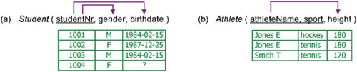
The table in Figure 14.58(b) is in 1NF but not 2NF, since height, a nonkey attribute, is functionally dependent on athletename, which is just part of the composite key. Notice the redundancy: the fact that Jones E has a height of 180 cm is recorded twice.

To avoid redundancy, we split the original Athlete table into two smaller ones, as in Figure 14.59. This figure shows both conceptual and relational schemas for the example (assuming that the information is mandatory for athletes). If you verbalized Figure 14.58(b) correctly in terms of elementary facts, you would obtain this conceptual schema directly, and the relational schema would follow automatically using Rmap.

You would have to be a real novice to verbalize Figure 14.58(b) in terms of a ternary, but suppose you did. The checks provided in the CSDP, especially steps 4 and 5, prompt you to discover that the functional fact type Athlete has Height. On seeing this, you would know to split the ternary into two binaries.

If you were careless in applying the CSDP, you could end up with the ternary in your relational schema. At this stage you could look for an FD coming from only part of a key, and use the 2NF normalization rule to at last correct your error. Even at this level, you should think in terms of the functional fact type behind the FD.

Recall that if fact types are elementary, all FDs are implied by UCs. This property is preserved by Rmap, since it groups together only functional fact types with a common key. So if we find an FD in a relational schema that is not implied by a UC, we must have gone wrong earlier. Since UCs imply FDs, every nonkey attribute is functionally dependent on any key of the relation. Note that to determine the hNF of a relation we need to be told what the relevant dependencies are (e.g., keys and FDs) or have a significant population from which these may be deduced.

Although normalization to 2NF overcomes the redundancy problem in the original Athlete table, this reduces the efficiency of those queries that now have to access both the new tables. For example, if we want the name and height of all the hockey players, the 2NF design means that two tables must be searched and their athleteName fields matched. This kind of efficiency loss, which is common to each normalization refinement (each involves splitting), is usually more than offset by the higher degree of data integrity resulting from the elimination of redundancy.

For example, if we need to change the height of Jones E to 182 cm, and record this change on only the first row of the original Athlete table, we now have two different values for the height. With more serious examples (e.g., defense, medical, business) such inconsistencies could prove disastrous.

As discussed in the next section, we may sometimes denormalize by introducing controlled redundancy to speed up queries. Although the redundancy is then safe, control of the redundancy is more expensive to enforce than in fully normalized tables, where redundancy is eliminated simply by enforcing key constraints. In short, normalization tends to make updates more efficient (by making constraints easier to enforce) while slowing down queries that now require additional table joins.

Given attributes X and Y (possibly composite), if X → Y, then an update of X entails a possible update of Y. Within a relation, a set of attributes is mutually independent if and only if none of the attributes is (functionally) dependent on any of the others. In this case the attributes may be updated independently of one another.

A table scheme is in third normal form (3NF) if and only if it is in 2NF and its nonkey attributes are mutually independent. Hence, in a 3NF table no FD can be transitively implied by two FDs, one of which is an FD between two nonkey attributes. For example, the table in Figure 14.60(a) is in 3NF since there is no dependency between gender and birthdate.

However the table in Figure 14.60(b) is not in 3NF, since population depends on birthcountry, and these are both nonkey attributes. Note that population is transitively dependent on the key (studentNr determines birthcountry, and birthcountry determines population). This table exhibits redundancy: the fact that the United States has a population of 301,139,947 is shown twice. To avoid this redundancy, the fact type underlying the FD between the nonkey attributes is split off to another table, as in Figure 14.61, which shows both ORM and relational schemas for the example.

Now consider the table in Figure 14.62, which is a modified version of an example used in Section 5.5 to illustrate the logical derivation check in the CSDP. If this CSDP step has been carried out properly, FDs from one nonkey attribute to another cannot arise in any tables obtained from Rmap. In the original Section 5.5 example, we split this table into two, one for the fact type Lecturer works for Department, and one for the fact type Department is located in Building, deriving the fact type Lecturer works in Building from the rule Lecturer works in Building iff Lecturer works for a Department that is located in Building.

However, if the “only” if part of the “iff” in this biconditional is not satisfied, then the two-table design loses information. For example, suppose that Wang and Zalewski do not work for any department (e.g., they might be visiting lecturers who work in some general office). This situation is represented by the last two table rows in Figure 14.62, using “?” to indicate a null. If we split the table in two as described earlier, it would be impossible to derive the facts about where Wang and Zelewski work.

The original work on normalization assumed that nulls do not occur, but this assumption is often false. If we agree with Codd (1990, p. 201) that nulls should be ignored when applying rules about FDs, then the FDs shown in Figure 14.62 still exist; but it is wrong to simply decompose this table into two, so this normalization step can be unsafe. Clearly, the safest way to deal with such issues is at the conceptual level.

Codd’s original definitions of 2NF and 3NF used “key” in the sense of primary key, so attributes of alternate keys were regarded as nonkey attributes. However, nowadays an attribute is termed a key attribute if it belongs to some key (primary or alternate), so a nonkey attribute belongs to no key.

Hence, in one sense the definition of 3NF does allow transitive dependencies if the intermediate attribute is a key. Consider the table in Figure 14.63. It has two keys. We could argue that the FD countrycode → population is transitively implied by the FDs coun-tryCode → countryName and countryName → population. Alternatively, we could argue that countryName → population is implied by countryName → countryCode and countryCode → population. However, the relation is still in 3NF as there is no FD between nonkey attributes. The ORM schema is shown at the left of the figure.

Let X and Y be attributes (possibly composite) of the same table. A functional dependency X → Y is trivial if and only if X contains Y. For example, the table scheme Student, studentNr, gender) has six trivial FDs: studentNr → studentNr, (studentNr, gender) → studentNr, etc. A functional dependency X → Y is full (rather than partial) if and only if there is no FD from just part of X to Y.

A full, nontrivial FD is said to be an elementary FD. Consider, for example, the table in Figure 14.64 about populations of U.S. cities (July 2006 figures). This has three elementary FDs that start at the primary key cityNr, and two elementary FDs that start at the alternate key (cityname, stateCode). Some nonelementary FDs in that table are cityNr → cityNr and (cityName, stateCode ) → cityName. We typically avoid displaying non-elementary FDs because they are obviously implied by the elementary FDs.

A key is an elementary key if there is an elementary FD from it to some attribute in the table. An attribute is an elementary key attribute just in case it belongs to some elementary key. For example, the city table in Figure 14.64 has two elementary keys cityNr and (cityName, stateCode). We may now define the next strongest normal form, which was proposed as an improvement on 3NF (Zaniolo 1982).

A table scheme is in elementary key normal form (EKNF) if and only if all its elementary FDs begin at whole keys or end at elementary key attributes. In other words, for every full, nontrivial FD of the form X → Y, either X is a key or Y is (part of) an elementary key. For example, the City table in Figure 14.64 is in EKNF. If the primary key of a table includes all its columns, the table is automatically in EKNF since it has no elementary FDs; for example: Enrollment (studentNr, subiectCode).

Now consider the OfficialLanguage table in Figure 14.65(a), which records the languages officially used in various countries. Countries may be identified by their codes or by their names. This table has two composite keys: (countryCode, language); (country-Name, language). The primary key is indicated by a double underline; since its attributes are not adjacent, a dotted line connector is added to show that this is a single, composite key rather than two simple key constraints. The secondary key is indicated by a single underline.

Since the OfficialLanguage table has no nonkey attributes, it is automatically in 3NF. However, it has obvious problems (e.g., the fact that the country with code ‘CA’ is named ‘Canada’ is duplicated). One way of spotting this bad design is to note that the table is not in EKNF. There is an FD from countryCode to countryName, and another FD from countryName to countryCode (depicted by arrows above the table). These elementary FDs come from parts of keys rather than whole keys, and these FDs do not end at elementary key attributes, since neither of the composite keys is elementary. So the table is not in EKNF.

The redundancy problem can be avoided by splitting the table into two EKNF tables as shown in Figure 14.65(b): Country countryCode, countrvName); LanguageUse( country-Code. language). The two FDs missed in the original table scheme are now captured by key constraints in the Country table, and the redundancy problem has been eliminated. The same design is obtained by Rmapping the ORM schema shown. If the language fact type is not mandatory for Country, replace the equality constraint in the relational schema by a simple subset constraint from LanguageUse.countryCode to Coun-try.countryCode.

The next normal form is named after Raymond Boyce and Edgar Codd, who proposed it as an improvement on the old 3NF. An equivalent definition was given earlier by Heath (1971). A table scheme is in Boyce-Codd Normal Form (BCNF) if and only if all its elementary FDs begin at whole keys (i.e., given any full, nontrivial FD X → Y, it must be that X is a key). For example, the relation scheme Student ( studentNr. gender, birthdate) is in EKNF because all its elementary FDs begin at the studentNr key. The only time that a relation can be in 3NF (or EKNF) but not in BCNF is when it has at least two candidate keys that overlap (Vincent and Srinivasan 1994).

Now consider the table in Figure 14.66(a). This is like the previous table, except that the percentage of the country’s population that actually uses the language is recorded (the figures here for Canada are fictitious). The keys are now elementary, since they functionally determine the percentUsage attribute. Since the FDs between countryCode and countryName now end at elementary key attributes, the table is in EKNF. But the table has the same redundancy as the previous table.

One way to spot this problem is to note that it is not in BCNF, since the FDs shown above the table do not start at whole keys. For instance, the functional dependency countryCode → countryName exists, but CountryCode is only part of the (countryCode, language) key.

The redundancy problem can be avoided by splitting the table into two BCNF tables, as shown in Figure 14.66(b). This design is automatically obtained by Rmapping the ORM schema shown. As before, if the language use fact type is optional, change the equality constraint to a subset constraint.

The principle underlying the refinement to second and third normal forms has been nicely summarized by Bill Kent (1983) as follows: “A nonkey field must provide a fact about the key, the whole key, and nothing but the key”. This should be refined by replacing “the key” by “a key”, and treated as a description of BCNF rather than 3NF.

In the previous two examples, a table with overlapping keys had to be split. Sometimes overlapping keys are permitted. Recall the example from Chapter 4 where students are assigned unique positions in subjects, with no ties. This leads to the BCNF table scheme

The previous normal forms considered only functional dependencies. The next normal form is due to Ronald Fagin (1977) and considers multivalued dependencies (MVDs). For a given relation with attributes X, Y, and Z (possibly composite), X mul-tidetermines Y (written as X → Y) if and only if the set of Y values is a function of X only (independent of the value of Z). In this case, Y is said to be multivalued dependent, or multidependent, on X; in such a case Z will also be multidependent on X. A functional dependency is a special case of an MVD, namely when the set of dependent values is a unit set. An MVD X → Y is trivial if and only if X includes Y, or X and Y together include all the attributes in the relation.

For example, the Athlete table considered earlier in Figure 14.58(b) is repeated in Figure 14.67(a), this time showing the nontrivial MVD athleteName → sport. As the ORM schema in Figure 14.67(b) indicates, MVDs usually arise from m:n associations. Although this poor design would be detected earlier because of its embedded FD (it is not even in 2NF), there are relations with MVDs that are in BCNF yet still have redundancy problems. To address such cases, we now consider the next normal form.

A relation is in fourth normal form (4NF) if and only if it is in BCNF and all its nontrivial dependencies are functional (single-valued) dependencies. So a 4NF relation cannot have any nontrivial MVDs that are not FDs. Basically, each nonfunctional MVD requires a separate table for itself.

Consider the Lecturer table in Figure 14.68(a). It is in BCNF since it is “all-key”. The table is not in 4NF since language and sport are each multidependent (but not functionally dependent) on surname. The MVDs are depicted as double arrows above the table. Assuming that the ternary means Lecturer plays Sport and speaks Language, the table exhibits redundancy. The facts that Halpin plays judo and karatedo and speaks English and Japanese are duplicated. To avoid this problem, the table is split into two 4NF tables (as obtained by Rmapping the ORM schema) as shown in Figure 14.68(c).

Now let’s delete the fourth row of this Lecturer table to obtain the smaller Lecturer table in Figure 14.68(b). Notice the question mark next to the MVDs. If we strictly apply Fagin’s definition of MVD, the relation (here a set of four tuples) does not exhibit these MVDs. According to Fagin (1977), the MVD X → Y holds for the relation R(X, Y, Z) if and only if whenever (x, y_h z{) and (x, y₂ , , Zi) are tuples of R, then so are (x, y_u z₂) and (x, y₂,, Z). By this definition, if the MVD surname → sport did apply, then the presence of the tuples (‘Halpin’, ‘karatedo’, ‘English’) and (‘Halpin’, ‘judo’, ‘Japanese’) requires the presence of the tuples (‘Halpin’, ‘judo’, ‘English’) and (‘Halpin’, ‘karatedo’, ‘Japanese’). But the second of these tuples is absent (we just deleted it). Similarly, the MVD surname →language does not apply because of this missing tuple. However even without these MVDs, the table shows fact redundancy (the facts that Halpin plays judo and speaks English still appear twice).

Clearly, what is important in practice is that the relation scheme be well designed, regardless of whether the current population of that scheme satisfies some required dependency. If somebody produced the table in Figure 14.68(b) the table would have no nontrivial MVDs according to Fagin’s definition, but the design is still faulty if the ternary means Lecturer plays Sport and speaks Language, since it allows fact redundancy.

For such reasons, we adopt the notion of what we call semantic 4NF, which relates MVDs to the meaning of the underlying fact types. If the ternary in Figure 14.68(b) means Lecturer plays Sport and speaks Language, then there is a semantic MVD surname → sport because, in terms of the underlying fact type Lecturer plays Sport, the set of sports is determined by the lecturer alone (without regard to language). Similarly there is a semantic MVD surname → language.

Suppose instead the ternary meant Lecturer plays Sport when it is conducted in Language. For example, Halpin might play judo only when it is conducted in English. In this case, the ternary is elementary so cannot be split without information loss. As this example shows, it is not in general possible to determine whether a table is well designed simply by inspecting its population(s). You also need to know what the table means.

ORM’s Rmap procedure forbids grouping two or more fact types with composite UCs (e.g., m:n associations) into the same table scheme, regardless of what the current populations might be. ORM’s notion of an alethic, static constraint refers to any possible population, and in principle requires an understanding of the business domain by the domain expert who asserts that such a constraint must apply. While sample populations can reveal the absence of a constraint, and provide hints as to the presence of constraints, they cannot guarantee that such constraints really do apply—such guarantees are the responsibility of the domain experts.

It can be shown that BCNF is equivalent to no redundancy when there are FDs, and 4NF is equivalent to no redundancy when there are FDs and MVDs (Vincent and Srinivasan 1993). Moreover, if a relation scheme is in BCNF and some key is simple, then it is also in 4NF (Date and Fagin 1992).

The next normal form is also due to Fagin (1979) and is based on join dependencies (JDs). A relation has a join dependency if it can be reconstructed without information loss by taking a join of some of its projections. If one of these projections is the table itself, this is a trivial join dependency.

A table is in fifth normal form (5NF) if and only if, for each nontrivial join dependency, each projection includes a key of the original table. A table is in project-join normal form (PJNF) just in case each JD is the result of the key constraints. Any 3NF relation scheme whose keys are all simple is also in PJNF (Date and Fagin 1992). The forms 5NF and PJNF are often treated as equivalent, but some subtle differences can be distinguished to show that PJNF is a stronger notion (Orlowska and Zhang 1992).

As an example of a key-based join dependency, Employee{ empNr. birthdate, gender) is equivalent to the join of the projections: Emp1( empNr. birthdate ); Emp2{ empNr. gender). The original table as well as the two smaller ones are all in 5NF. Since a relational schema is in a given normal form if its table schemes are all in that form, a relational schema that includes just the Empl and Emp2 tables is a 5NF schema. This illustrates that 5NF of itself does not guarantee that a schema is minimal with respect to the number of tables.

Nontrivial join dependencies that are not key-based are rare, so 4NF tables are almost always in 5NF as well. The theory underlying the test for 5NF was included in the projection-join check at CSDP step 4, so we confine ourselves here to a brief discussion. A classic example used to discuss the notion is portrayed in the SellsFor table in Figure 14.69(a). A small sample population is provided to show that the only uniqueness constraint is the weakest possible (verify this for yourself).

Conceptually, this ternary fact type may be expressed as: Agent sells Cartype for Company. The fact types behind the three binary projections may be expressed as: Agent sells Cartype; Agent represents Company; Company makes Cartype. Any attempt to split this ternary into two binaries will result in information loss. For example, from the facts that Smith is a representative for Foord, and Foord makes a four-wheel drive (4WD), it does not follow that Smith sells a 4WD.

However, the population of the SellsFor table does equal the join of the three binary projections (confirm this for yourself). So we could split this particular table population into three binary table populations without information loss.

But since database populations are updated continually, if we are to split the table scheme into three binary table schemes, we need to know that this join dependency applies to all possible, complete populations. In other words, is the sample population significant in this regard? If it is, the derivation rule shown in Figure 14.69(b) applies.

The only way to check that this is an actual business rule is to ask the domain expert. Let’s suppose that it’s not a rule. For example, it is now acceptable to delete just the first row of the SellsFor table in Figure 14.69(b). Check for yourself that this deletion should be rejected if the rule did apply. In this case, the ternary fact type is elementary and should be left as it is. If the derivation rale does not apply, the SellsFor table scheme is already in 5NF.

Now suppose the derivation rule does apply, as shown in Figure 14.69(b). This rule needs to be enforced, but the key constraint in the SellsFor ternary fails to do this (e.g., it allows the first row to be deleted). To avoid this problem, the 4NF ternary should be split into three 5NF binaries, as shown in Figure 14.69(c). If some of the roles in the ORM schema are mandatory, some inter-table constraints need to be added. If desired, the original ternary may be defined as a view derived from the join of the new tables.

It has been argued (e.g., by Kent) that when relation schemes such as SellsFor in Figure 14.69(a) are elementary, there is a kind of “unavoidable redundancy”. For example, the “fact” that agent ‘Jones E’ sells sedans is repeated on rows 1 and 3. However, such “redundancy” is harmless because it is derived rather than stored. Although the tuple (’Jones E’, ‘sedan’) is stored twice, the fact that agent ‘Jones E’ sells sedans can only be obtained via the derivation rule Agent sells Cartype iff Agent sells Cartype for Company.

The seven normal forms discussed so far are strictly ordered. Each higher normal form satisfies the lower forms. Recall that “⊂” denotes “is a proper subset of. Let “5NF-rels” denote the set of all possible relations in fifth normal form, and so on. The strict ordering may now be set out thus (in decreasing order of normality):

5NF-rels ⊂ 4NF-rels ⊂ BCNF-rels ⊂ EKNF-rels ⊂ 3NF-rels ⊂ 2NF-rels ⊂ 1NF-rels

Essentially, normalization through to 5NF simplifies table updates by ensuring that three kinds of dependency (FDs, MVDs, and JDs) will automatically be enforced by key constraints (i.e., uniqueness constraints within each table). An FD is a special case of an MVD, which in turn is a special case of a JD. As noted by Fagin, BCNF ensures that all FDs are implied by key constraints, 4NF ensures that all MVDs are implied by key constraints, and 5NF ensures that all JDs are implied by key constraints.

The last normal form we consider is domain key normal form (DKNF), which was introduced by Fagin (1981). A table scheme is said to be in DKNF if and only if all its constraints are expressible as domain dependencies or key dependencies. A domain dependency specifies a set of possible values for a given attribute. This basically declares a data type (e.g., varchar(20)) or a value constraint (e.g., {’M’, ‘F’}) for the attribute. A key dependency is a uniqueness constraint spanning one or more attributes in the table scheme. If all domains are infinite, any DKNF table scheme is also in 5NF.

For a relational database schema to be in DKNF, each of its table schemes should be in DKNF, and there should be either no intertable constraints or only “simple” intertable constraints that are easily enforced, such as inclusion dependencies (subset constraints).

DKNF designs are easy to understand, and their constraints can normally be efficiently enforced by a DBMS. Unfortunately, however, life is not so simple. Many other kinds of constraint often arise in practical applications, and need to be enforced even though their inclusion in the relational schema violates DKNF.

As a simple example, Figure 14.70 shows a conceptual schema and its relational mapping. The table scheme Person is not in DKNF because it contains two constraints other than domain and key dependencies. First, the subset constraint from manager to personNr is an intratable inclusion dependency. Second, the “personNr ≠ manager” constraint enforces the irreflexive nature of the reporting association. The overall schema is not in DKNF because its Person scheme is not in DKNF, and because of the intertable exclusion constraint (no person wrote and reviewed the same book).

Although the relational schema in Figure 14.70 is not in DKNF, each of its table schemes is in 5NF. The additional constraints are simply not included in the definition of 5NF so do not violate it. Any valid ORM schema, where each asserted fact type is atomic, will result in a 5NF relational schema if mapped according to our Rmap procedure.

As this example shows, ORM actually goes beyond 5NF by catering for other kinds of constraint. Although this rich support for expressing and mapping constraints may lead to schemas that violate DKNF, that’s actually an advantage rather than a weakness, since such violations are needed to capture the relevant business rules.

It is very common to encounter cases where normalization to 5NF or DKNF fails to fully capture the relevant constraints. A modified version of an awkward but classic example is set out in Table 14.8. In this UoD, lecturers are assigned exactly one subject, and this is the only course they may teach.

Table 14.8. An unusual and awkward example.

Lecturer	Course	Student
Halpin	CS113	Brown A
Rose	CS102	Brown A
Nijssen	CS113	Smith J
Rose	CS102	Smith J
Halpin	CS113	Wang J
Bloggs	CS226	?

The null indicates that Bloggs does not teach the assigned course (e.g., because too few enrolled for it). For each course they take, students have exactly one lecturer. The same course may have many assigned lecturers. Because of its strange constraint pattern, this example is not easy to verbalize in elementary facts on a first attempt. You are invited to try this before reading on.

An initial conceptual schema based on one verbalization is depicted in Figure 14.71(a). If this is the global schema, the mandatory role constraints are implied by the pair-subset constraint. More importantly, the uniqueness constraint on the binary when combined with the pair-subset constraint has other implications. Can you spot these?

The pair-subset constraint indicates that lecturers may teach only their assigned courses, but the uniqueness constraint on the binary indicates that each lecturer is assigned at most one course. Hence lecturers may teach at most one course. So there is an FD from the first role of the ternary to the second role, as shown in Figure 14.71(b). Since the ternary has an implied, spanning UC, the implied FD implies the UC across the first and third roles. Moreover, since there is a third role in the ternary, the fact type now cannot be elementary. This is an example of the general rule set out in Figure 14.72. Two corollaries are included, one of which we will make use of in our example. You may wish to prove these corollaries as an exercise.

If a fact type is elementary, all its FDs are the result of its UCs. If another FD exists, then semantically underlying this FD is another fact type, which is the target of a pair-subset constraint from the original fact type. If this is expressed at the conceptual level, we know the original fact type is not elementary and should remove the relevant role (as in Figure 14.72).

The ternary in Figure 14.72 matches this pattern, but has an additional UC across its last two roles (for each subject, a student has only one lecturer). To preserve this constraint after removing the role, an external UC must be added between the course and student roles in the new schema (see Figure 14.73).

The general requirement for this extra move is specified as the first corollary in Figure 14.72. When the corrected conceptual schema is Rmapped, we obtain two table schemes with two intertable constraints (Figure 14.73).

Suppose that instead of dealing with Table 14.8 conceptually, we develop a relational schema for it using the normal form theory discussed earlier. We might begin with a single ternary: Teaches (lecturer, course, [student]). Suppose that someone now tells us all the constraints or cleverly constructs a significant population from which the constraints can be deduced. We note that there are two composite uniqueness constraints over (lecturer, student) and (course, student). Since student is an optional attribute, neither of these can be used as a primary key, so we know something is wrong (although the normal form theory discussed earlier ignored nulls). Indeed we know the table is not in BCNF since we have the FD lecturer → course, and lecturer is not a key.

At this stage we split the table into two: Assignee (lecturer, course); Instruct (lecturer, student ). These are the same two tables we arrived at by deconceptualization in Figure 14.73. However, the normal form theory discussed in this section tells us nothing about the two intertable constraints. We have to figure these out for ourselves.

Further normal forms could be invented to cater for further constraints, but surely it is better to focus on cleaning up design faults at the conceptual level where humans can utilize their semantic understanding of the UoD more easily.

As discussed in the next section, it is sometimes necessary to denormalize a relational schema in order to achieve acceptable performance. This is a possible option for the current example. Note that the intertable constraints are expensive to enforce, unlike key constraints. For example, enforcing the external uniqueness constraint effectively requires a table join each time a row is inserted into either table. Moreover, queries to list who teaches what to whom need a table join.

Another design is obtained by mapping the original ORM schema in Figure 14.71(a) to give the relational schema shown in Figure 14.74(a). The pair-subset constraint implies the ternary’s other key constraint on (lecturer, student), which may thus be omitted. Although the ternary is denormalized, it is safe since its problematic FD is enforced by the pair-subset constraint and the key constraint in the binary. We may now list who teaches what to whom, without a table join. If this is a focused query for the application, this design might be preferred.

To modify the example somewhat, suppose lecturers must teach the course assigned to them (so the null in Table 14.8 cannot occur). Figure 14.71(a) is changed to make both roles of Lecturer mandatory, with the subset constraint becoming an equality constraint, and Figure 14.73 is changed to make both roles of Lecturer mandatory, and the relational subset constraint becomes an equality constraint.

If the normalized, two-table design has poor performance, we might denormalize the design to a single table that is their natural join, as shown in Figure 14.74(b). With the subset constraint of Figure 14.71(a) replaced by an equality constraint, assignment facts can be retrieved by projecting on the first two roles of the ternary, but the uniqueness constraint on the assignment binary still needs to be catered for. In the de-normalized ternary, this constraint cannot be enforced as a uniqueness constraint, so a separate constraint is required to enforce the FD lecturer → course. As long as this additional constraint is enforced (e.g., as a user-defined constraint in SQL), the single-table design is safe. As before, the alternate key constraint is implied and hence omitted.

Advances in relational languages are making it easier to specify constraints such as FDs that are not key based. However the overhead of enforcing such constraints needs to factored in when choosing the final relational design. In general, we should first try a fully normalized design, using conceptual optimization where relevant to improve it. If performance is still unacceptable, controlled denormalization is an option.

Exercise 14.6

1.	The conceptual schema for a given UoD is as shown. Some table schemes designed by novices for parts of this UoD are listed here. Indicate briefly, in terms of normalization theory, why each of these table schemes is not fully normalized. Parenthood ( parentName. gender, Child( childName, gender )) Teaches ( person. subjectTutored. [subjectLectured]) ParentOf{ parent, child. genderOfParent, genderOfChild ) Tutor (tutorName. subject, [child!) Use Rmap to generate a correct relational schema.
2.	The conceptual schema of Question 1 is incomplete with respect to real-world constraints. For example, parents of the same child must differ in gender, but this constraint is not captured. Replace the parent predicate with mother and father predicates, to develop a more complete schema that includes this constraint (Hint: include subtyping). Rmap your solution to (a).
3.	Suppose that while developing a conceptual schema you specify the following fact type: Manager supervises Trainee on Project. Assume that no manager is a trainee, and that all objects are simply identified by name. The following constraint applies: no manager may supervise the same trainee on more than one project. Draw this as a ternary fact type, including the constraint. You now check whether there are any other functional fact types of interest between these object types, and discover that each manager supervises at most one project. Add this fact type to your schema and then add any set-comparison constraint that applies. Is the ternary elementary? If not, explain why not, and correct the schema. The following business rule is now added: each trainee on a given project has only one supervisor for that project. Add this constraint to your schema. Rmap your answer to (d). Because of poor performance, this relational schema is regarded as unsatisfactory. Using controlled denormalization, suggest an alternative relational schema.