
15.5. Modeling Information Dynamics in UML
The UML includes a range of different diagram types—13 types in all in UML Version 2 (an increase over the nine types available in UML Version 1). Figure 15.32 shows the range of diagram types: boxes with dashed lines are simply summary supertypes and not actual types of diagram.
Figure 15.32. UML 2 diagram types.

UML supports information modeling through class diagrams and, to a lesser extent, object diagrams. These have been covered in some detail elsewhere in this book and we won’t discuss them again here. UML also has several diagram types that can be used to model behavior.
The four types of interaction diagram shown in Figure 15.32 are mainly of interest in software development and have limited application in business modeling. Sequence diagrams and communication diagrams describe messages passed between object instances. Interaction overview diagrams are a specialized variant of activity diagrams—we discuss activity diagrams in more detail shortly. Timing diagrams show the detailed timing of interactions between various system elements and are mostly only relevant to real-time systems.
We first take a very brief look at use case diagrams. A use case describes a connected series of actions performed by one or more actors in relation to the system under discussion. An actor may be human or machine, but, by convention, both are shown graphically as a stick figure icon. The use case description is usually expressed from the viewpoint of one particular actor—the principal actor. A use case diagram contains none of this description and is essentially no more than a list of the relationships between actors and use cases (and sometimes between use case and use case), depicted in a graphical rather than a tabular form. A simple example is shown in Figure 15.33.
Figure 15.33. A simple use case diagram for an automated teller system.
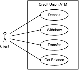
The oval shapes in Figure 15.33 represent use cases. These are usually named with a verb phrase that summarizes the actions being performed in the use case. The optional rectangular boundary represents the system, which is slightly misleading since the use case describes the actor’s interactions with the system (i.e., the use case is not “in” the system).
The UML standard describes various extensions to the basic concept. For instance, some shared activity that potentially appears in several use cases can be extracted out into a separate use case and referenced by an «include» relationship. Some activity that only occurs in exceptional cases can be separated out into a separate use case and referenced in an «extend» relationship.
Actors and use cases can be treated as classes, with subtyping used to show hierarchical relationships between actors and between use cases. However, these and other elaborations often end up causing more problems than they solve and should be used with caution. The valuable part of a use case is the actual behavioral information contained in the use case description, but, strangely, this aspect is not defined in UML.
A common error is to equate a use case with a business process. This may be true in very small systems, but in most major enterprises, cross-functional business processes span many organizational units. This makes it unlikely that individual actors (from whose perspective the use case is being described) will see the whole of the process. It is more likely that a use case describes a segment of a process, as shown in Figure 15.34 (note: this figure is not a UML use case diagram!).
Figure 15.34. Relationship between use cases and processes.

Use cases that overlap in their descriptions (as do UC2 and UC3 in Figure 15.34) should corroborate each other. If not, further investigation is required. Gaps in the coverage of the process (as between UC3 and UC4 in Figure 15.34) also require investigation. Perhaps we have a missing use case? Or perhaps our understanding of the process is not correct?
Although use cases can help uncover some dynamic aspects of business information, they are not sufficiently rigorous to be our primary modeling tool, and they are best seen as a step on the path to producing a more comprehensive and precise business model. The remaining two UML behavioral diagram types can be pressed into service to model dynamic business behavior, and we will look in a little more detail at some of their features.
Activity Diagrams
Activity diagrams are mainly focused on the flow of control within a set of related activities. The level of granularity is not defined by UML, so the scope of each individual activity is at the discretion of the modeler. This has the advantage that activity diagrams can be used for both high level and low level descriptions, but places the onus of defining activity boundaries onto some other authority. Activities are considered to be composed of atomic actions. Activities can be interrupted, but actions cannot, which implies that any interruption to an activity must take place on a boundary between actions. We have already seen flow-of-control chaining of activities earlier in this chapter, and it’s not surprising that UML activity diagrams are seen as a candidate notation for documenting business processes. The underlying semantics of activity diagrams changed between UML versions 1 and 2. In UML 1, activity diagrams were seen as a special kind of state machine description and shared a great deal of terminology with UML statecharts. In UML 2, the semantics of activity diagrams became realigned to be closer to the semantics of Petri nets.
An activity diagram consists of a number of nodes connected by arrowed lines (directed edges). There are three main types of node: action nodes, object nodes, and control nodes. Action nodes represent some work being carried out and are shown as a rectangle with rounded corners. The rectangle typically contains the name of the action: other information may optionally be added that we won’t consider here. Object nodes, shown as rectangles with square corners, represent an object type, for example, a business entity such as an invoice that may be passed from one activity to another. Object nodes are generally only shown when some special consideration needs to be given to the objects being passed: routine use of business objects by activities is just assumed. The “flow” along the activity edges is either of control tokens, indicating the transfer of control from one activity to another, or of objects. Since the edges are directed, there is no assumed direction of flow, although diagrams are conventionally laid out so that the main flows are either left to right or top to bottom.
Control nodes are abstract activity nodes that coordinate flows in an activity diagram and come in various subtypes. An initial node is represented by a filled circle and represents a starting point for the activity diagram. There can be more than one initial node. There are two kinds of final node. An activity final node is shown as a target symbol, and an activity diagram can have more than one of these. As soon as an activity final node receives a token, the entire activity immediately terminates even if there are other control tokens active in other paths. A flow final node, shown as an “X” in a circle, destroys any token that reaches it, without affecting any other concurrent flows.
A decision node, denoted by a diamond shape, has one input edge and one or more output edges. A token arriving on the input edge will leave on only one of the output edges (i.e., exclusive-or). To control this, the output edges have guard conditions, denoted inside square brackets. The guard conditions should be complete and disjoint to ensure that token flow is not inadvertently halted or duplicated. A default branch can be provided by specifying it with the guard condition [else].
The diamond shape used for a decision node is also used for a merge node. This performs the complementary action to a decision node by bringing together multiple alternate flows on its input edges. Any token arriving on an input edge is offered to the output edge. There is no synchronization of tokens arriving on the incoming edges.
A fork node splits a flow into multiple concurrent flows. It is shown as a solid bar with one input edge and two or more output edges. Each token arriving on the input edge is duplicated and offered to each output edge. There is no sequencing implied between the outgoing flows.
A join node is used to combine parallel flow paths. The join notation is the same as for a fork, except that the join has multiple input edges and one output edge. An optional join expression determines how incoming tokens are combined to produce an output token. The default is “and”, implying that the join waits for a token to arrive on each incoming edge before producing a token on the output edge (i.e., synchronization).
The UML 2 specification does not require that branches introduced in the diagram should be balanced. In other words, multiple paths introduced by decisions or forks do not necessarily have to be recombined by the complementary merges or joins. Although this provides maximum flexibility in defining a process, it can also provide subtle traps for the unwary and can lead to unsound process definitions.
Figure 15.35 shows an example activity diagram for a simple sales process. The diagram is based on an example given in the UML specification, modified slightly to contain examples of the features we discuss. Although the modified diagram is still syntactically legal, it represents an unsafe process design, as we will see shortly. The diagram is self-explanatory, but not unique, in the sense that the same process could have been depicted in a number of slightly different ways.

For example, the join and the fork that immediately follow it could have been combined into a join/fork construct that would have appeared as a thick bar with two edges entering and two edges leaving. Combining a join and a fork in this way can make diagrams slightly tidier, but has no effect on the semantics.
The execution of the process can be simulated by tracing the flow of a token in a particular instance of the process represented by the diagram. The token originates at the initial node. A customer places an order, which is received by the company’s sales department. The first decision is to either accept or reject the order. The two guard conditions, [rejected] and [accepted], are mutually exclusive. If the token takes the [rejected] branch, it immediately reaches the merge and appears on its output edge. After the order is closed, the token reaches the activity final node, which immediately ends the process instance. If the token takes the [accepted] branch, the order is filled. When the token reaches the fork, two tokens are generated. The upper token causes the order to be shipped, and the lower token stimulates a series of actions to invoice the customer and eventually receive payment.
The upper and lower branches have no implied timing constraints: either of them could be the first to complete. The following join waits for a token to arrive on both branches before emitting its own single token. This immediately forks into two other branches. The token on the upper branch reaches the merge that we have already discussed and causes the order to be closed. The token on the lower branch reaches a decision. If the customer is a new customer, then they are added to the customer database, but for an existing customer the token is immediately consumed by the flow final node.
The second fork in the diagram is not balanced (there is no corresponding join), but we eliminate the token in the lower branch because it eventually reaches a flow final node. This ensures that adding the customer to the database does not interfere with the closing of the order. However, the design is unsound because the lower branch is in a race with the upper branch. Once the order is closed, a token will reach the activity final node and immediately terminate the process, regardless of the status of the token in the other branch. This could result in a new customer not being added to the database, contradicting the process designer’s original intentions.
One other feature of activity diagrams is support for swimlanes. These are optional, but can be used to indicate features such as separation of responsibilities, usage of resources, geographical distribution, and so on. As with other features, the precise meaning of a swimlane is not defined in UML: the interpretation is left up to the user of the activity diagram. Figure 15.36 shows the process model of Figure 15.35 with swim-lanes added. In Figure 15.36 the swimlanes are drawn to indicate who carries out the actions (customer or sales clerk). The invoice object is used by both, and so is shown on a swimlane boundary. Multiple orthogonal swimlanes can be defined: for example, one axis could represent organizational units and the other could represent resource types. The result resembles a kind of Venn diagram with the actions placed in whichever swimlane intersection is appropriate. However, this quickly gets difficult to draw and can be confusing to read.

Activity diagrams also provide for the hierarchical composition/decomposition of actions. A structured activity of this kind can be treated at one level as a single action, but can be expanded if required to show the breakdown into its subordinate activities. Activities can be nested in this way to any level that’s useful.
Activity diagrams have a number of other features that we haven’t space to discuss here. Examples include signaling between system elements, events used to trigger activities, the definition of interrupts and interruptible regions of activity, and so on. Many of these features can be useful in the definition of software, but are less relevant for conceptual modeling.
State Machine Diagrams
In UML version 1, state machine diagrams were known as statecharts and were closely aligned with activity diagrams, to the extent that an activity diagram could be considered as a special type of statechart. In UML version 2, state machine diagrams and activity diagrams occupy positions that are rather more distinct.
UML state machine diagrams have many of the same main constituents as other state diagramming conventions. States are normally shown as rectangles with rounded corners. The name of the state can be shown free-form inside the rectangle, in a separate compartment in the rectangle, or as a name tag attached to the rectangle, as shown in Figure 15.37.
Figure 15.37. Alternative state notations in UML.

States are interconnected by transitions, shown as directed lines. The lines typically begin on the border of one state and end on the border of another state—we discuss some special cases later. A transition can begin and end at the same state, and it’s possible for there to be more than one transition between a particular pair of states.
A state can be simple or composite. Composite states contain other substates within them. If a state has an active substate, then the containing state is also active. A composite state that is subdivided into multiple regions is known as an orthogonal state. Figure 15.38 shows examples of a simple composite state (containing exactly one region) and an orthogonal state (in this case, with two regions).
Figure 15.38. (a) Simple composite state, (b) Orthogonal state.
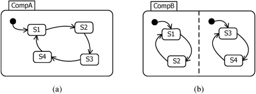
The small black nodes in Figure 15.38 are special pseudostates that represent the initial conditions for their respective states. Within a region, only one substate can be active at any one time, so the state shown in Figure 15.38(a) can be in state SI or S2 or S3 or S4. In contrast, the state shown in Figure 15.38(b) can be in state SI or S2 and also in state S3 or S4. A state can also contain nested state machines—called submachine state machines—which are semantically equivalent to composite states. Subma-chines are a convenient way of encapsulating common behaviors for reuse.
Actions can be carried out in a state at one of three times:
on entry to the state, denoted as entry / action
during the state (perhaps continuously in a loop), denoted as do / action
on exit from the state, denoted as exit / action.
All of these are optional. The “during” actions do not begin until any entry actions are completed and will be completed or aborted before any exit actions begin. This ensures that entry actions are always carried out before anything else and that exit actions are always carried out after anything else. Actions carried out within a state correspond to the Moore machine semantics discussed earlier. If required, the actions can be shown on a state machine diagram by listing them in a compartment of the state symbol just below the compartment with the state name, as shown in Figure 15.39.
Figure 15.39. Showing state actions.

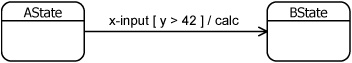
Transitions between states can have a label that consists of up to three parts. The normal notation is: e [g] /a, where
| e | identifies the triggering event causing the transition (the event may have parameters), |
| g | is a guard expression, enclosed in square brackets, and |
| a | identifies a list of one or more actions, preceded by a “slash” character. |
All three components are optional, so zero, one, two, or all three of the components could be present. Figure 15.40 shows a typical transition with all three components present.
Figure 15.40. A labeled transition.
If no event is specified, the transition is enabled when the actions in the preceding state have completed (a completion transition). If a guard expression is specified, it must evaluate to “True” for the transition to be taken. The guard expression is evaluated at the point in time that the transition is about to be taken. If it evaluates to “False”, the transition will not be taken, even if it has been enabled by an event. If actions are specified on the transition, they are completed before entering the target state. This corresponds to the Mealy machine semantics discussed earlier. UML state machines can therefore take on the characteristics of a Moore machine, a Mealy machine, or both.
Events are handled by a state machine one at a time, with run-to-completion semantics. This means that an event is only recognized and processed after the processing of the previous event is fully completed. This simplifies the state machine because it can never get into a situation of processing an event while it is in some intermediate configuration (e.g., part way through a transition from one state to another). Events do not necessarily cause transitions: an event can be recognized and processed within a state. Events can also be recognized but deferred in a particular state. A deferred event is saved and passed to the following state, where it must be either accepted or deferred once again. This continues until the event is no longer deferred or is where it triggers a transition.
UML defines a number of pseudostates that can be either the source or the target of a transition. The notations used for each of the pseudostates are listed in Table 15.3.
Table 15.3. UML pseudostates.

The initial pseudostate is the source for a single transition to the default state of a composite state. There can be at most one initial pseudostate per region. A final pseudostate indicates completion of its containing region. The containing state for a region is considered completed when all of its contained regions are completed. If all regions contained in a state machine are completed, then the entire state machine terminates. This is equivalent to destroying the object (in the programming sense!) with which the state machine is associated.
An entry point provides for the entry to a state machine or composite state that targets a specific state within the enclosing region. The entry actions associated with the enclosing state are executed before the transition to the enclosed state. A transition that enters an exit point implies an exit from the enclosing state machine or composite state. Any exit behavior of the enclosing state is executed after the transition from the enclosed state. Entry and exit points can be shown within the boundary of a state or on the boundary line of the state.
Junction pseudostates are used to combine together multiple transitions and/or to split a transition into several branches, each with a different guard condition. The latter case is known as a static conditional branch. A choice pseudostate is a dynamic conditional branch—it evaluates the guards on its outgoing transitions dynamically so as to reflect the results of actions performed in the same run-to-completion step.
Fork pseudostates split transitions that are targeted at states in different orthogonal regions. Join pseudostates perform the complementary operation of combining transitions that originate from states in different orthogonal regions.
A transition entering a deepHistory pseudostate restores the most recently active configuration of the composite state and all its substates. A transition into a shallow-History state is similar, except that the configurations of any substates are not restored.
A composite state can have at most one deepHistory pseudostate and at most one shallowHistory pseudostate, In either case, if the composite state had not been active previously (i.e., it has no history), the outgoing transition from the history state is taken.
Entering a terminate pseudostate implies that the execution of the containing state machine is terminated. This is equivalent to destroying the object with which the state machine is associated—again “destruction” is intended here in the programming sense.
In a hierarchical state machine, more than one state can be active at the same time. If a nested state is active, then its parent state and all of its ancestors back to the top-level state are also active. There can be at most one active state in any one region. An orthogonal state can have an active state in each of its regions. Entering an orthogonal state implies entering each of its regions (explicitly or by default). Similarly, exiting an orthogonal state implies exiting all of its regions.
It’s sometimes convenient to hide the decomposition of a composite state: suppressing selected details can allow attention to be focused on larger issues. A composite state with a hidden decomposition is shown graphically by adding a small icon to the state that looks like two horizontally placed states with a connecting line, illustrated in Figure 15.41. A tool that supports state modeling would typically have some convenient mechanism for expanding back to the detailed view of the composite state. Hiding detail in this way does not change the state model, only the way that it is displayed.
Figure 15.41. A state with a hidden decomposition.

We’ve glossed over some of the finer details of how state machines are defined in UML. For instance, there are situations that lead to nondeterministic results. One example is two transitions exiting the same state, triggered by the same event, but with different guard conditions. If the guard conditions overlap so that both evaluate to “True”, both of the transitions are enabled but only one of them will fire. In such cases the algorithm for selecting which transition to fire is determined by the implementation. If guards on transition branches are framed so that it is possible for all guards to simultaneously evaluate to “False”, the model is considered ill-formed. A simple cure for this latter situation is to include a branch with the guard [else], which will be chosen if the guards on all the other branches evaluate to “False”. Another complex area is the processing of events in state machines that have extensive nesting of substates. A given event may be relevant to several substates, but deciding which one actually gets to process the event is not a trivial exercise.
State machines are very popular with some users of UML, but most of these appear to be in application areas dominated by either real-time constraints or the need to be highly reactive to external events. In a typical business information system, time constraints are less onerous: a processing delay is more likely to be annoying than fatal. Historically, business systems were also less concerned with being reactive: in fact, early batch processing systems could hardly be said to be reactive at all. With the increasing trend toward online processing, reactivity is becoming more important. Anecdotal reports on the use of state machines in business applications suggest that business people find state-based descriptions less intuitive than process-based descriptions. It also seems to be true that a large proportion of the developers of business software are unfamiliar with the basic concepts of state machines. However, state machines do offer some powerful capabilities: in particular, the ability to generate application code from suitably constructed models. The next section discusses one approach that relies on state modeling to provide the behavioral aspects of an executable specification.
Executable UML
As the name suggests, Executable UML is a dialect of UML that is focused on a style of modeling that results in a model that can be compiled and executed. It is based on a fusion of ideas from the earlier Shlaer-Mellor methodology and standard UML. An executable UML model is built around three core concepts: specifying structural aspects, such as data, using UML class diagrams; specifying dynamic behavior and control using state machine diagrams; and specifying actions using an action language. The use of class diagrams and state diagrams is close to standard UML, but with a few detailed differences. At present, UML does not define any notation or syntax for an action language, although there is a specification for the semantics that must be supported by such a language. The consequence is that each variant of Executable UML has its own language. A proposal for standardizing an action language is currently in progress within the OMG.
The first stage of analysis separates different areas of concern into different domains to be modeled. A domain contains a set of cohesive concepts that can be considered without requiring detailed knowledge of other domains. Domains are interconnected by bridges that resolve intercommunications required between domains. The assumptions made in one domain can form the requirements for another domain. For example, a business-related domain may assume the existence of a communication network with certain characteristics. These business domain assumptions contribute to the requirements for the communication network domain. Bridges allow separation of concerns, so, for example, the elements in a business domain can be developed and refined without considering the details of any technical domain. This also makes the system design more resilient. For instance, modification to a technical domain does not necessarily have to impact a business domain, so we could “unplug” one technical realization and “plug in” a different one without impacting the business, as long as we can define a suitable bridge.
The functionality required in a domain can be established in any desired way. We assume here that this is done through use case analysis. The information contained in the use case descriptions can be dissected to determine an initial set of classes. It’s likely that the initial class definitions will be extended and refined many times as the design progresses.
Associations between classes on a class diagram are handled in a slightly different way from standard UML: each association is given a unique identifier and the association ends are named with verb phrases instead of the noun phrases of standard UML. Classes have operations defined in the usual way. These operations typically compute and return some value, or create, delete or modify some object (or perhaps a combination of these). Each instance of a class (i.e., an object) has a life cycle. For some classes, the behavior of their instances does not vary. An object is created, it reacts in a fixed way to any stimulus (a call to one of its operations) and eventually it goes away—not a very exciting life cycle. Other classes have behaviors that change over time, depending on the history of events to which the object has reacted. For these classes, a state machine can be defined to model their life cycle. State machines in most implementations of Executable UML adopt a subset of the possibilities defined in the UML specification. In particular, actions are typically encapsulated into procedures that are executed on entry to a state (standard UML allows other possibilities).
The procedures are defined in an action language. The language is at a higher level of abstraction than standard programming languages such as C# or Java in order to remove dependence on a particular software platform. Action language statements are conceptually concurrent: decisions about how to serialize these are left to the model compiler. Similarly, such concerns as data access, persistence, distribution, and so on are not specified in the action language. The only direct manipulation that can be specified in an action language is manipulation of the model elements themselves. At the time the model is compiled, the action language specification can be mapped onto the desired architecture. In principle, the same model could therefore be used in an embedded system, a Web service, a distributed application, and so on.
Executable UML has been applied successfully in a variety of applications. Most of these are real-time applications that lend themselves very naturally to state-based specification. Products are available from a small number of vendors who tend to be focused on the reactive systems market. However, there seems to be no reason why the concepts should not be equally applicable to general business systems, so the current focus may just be a reflection of historical market positioning, rather than any inherent feature of the technical approach.