3.4. CSDP Step 2: Draw Fact Types and Populate
Once we have translated the information examples into elementary facts, and performed quality checks, we are ready for the next step in the conceptual schema design procedure. Here we draw a conceptual schema diagram that shows all the fact types. This illustrates the relevant object types, predicates and reference schemes. Once the diagram is drawn, we check it with a sample population.
|
CSDP step 2: Draw the fact types and apply a population check. |
Consider the sample output report of Table 3.6. Let us agree that the information in this report can be expressed by the following three elementary facts, using “regNr” to abbreviate “registration number”:
The Person named ‘Adams B’ drives the Car with regNr ‘235PZN’.
The Person named ‘Jones E’ drives the Car with regNr ‘235PZN’.
The Person named ‘Jones E’ drives the Car with regNr ‘108AAQ’.
Table 3.6. A relational table listing who drives what cars.

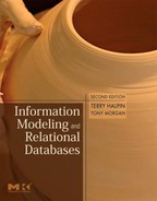
Before looking at the relevant conceptual schema diagram, it may help to explain things if we first view an instance diagram for this example (see Figure 3.8).
Figure 3.8. An instance diagram.
Instance diagrams illustrate particular instances of objects and relationships. Taking advantage of the concrete nature of the entities in this example, cartoon drawings denote the actual people and cars. The values are shown as character strings. A particular fact or relationship between a person and a car is shown as a solid line. A particular reference between a value and an entity is shown as a broken line.
Figure 3.9(a) shows a conceptual schema diagram for the same example, adding inverse readings for the two fact types. Instance diagrams and conceptual schema diagrams depict an entity type as a named, solid, soft rectangle (rectangle with rounded corners). A value type is shown as a named, broken, soft rectangle. The object type’s name is written inside. Some versions of ORM allow an ellipse (Figure 3.9(b)) or a hard rectangle (Figure 3.9(c)) instead of a soft rectangle.
Figure 3.9. (a) A conceptual schema diagram (minus constraints), and (b and c) alternate shapes.

On an instance diagram, individual objects are portrayed explicitly (by icons or text). However on a conceptual schema diagram, individual objects are omitted (unless we reference them in associated tables). Recalling that a type is the set of permitted instances, we may imagine that objects are represented as points inside the type shape.
On a conceptual schema diagram, the roles (relationship parts) played by objects are shown explicitly as boxes. Optionally, roles may be given a name, in which case the role name is displayed in square brackets next to the role box, for example, “[driver]” in Figure 3.9(a). Each predicate is depicted as a named, contiguous sequence of one or more role boxes (”contiguous” means the boxes are adjacent, with no gaps in between).
Predicates are typically ordered from one end to the other, with their reading displayed next to the predicate shape. For binary relationships (2 roles), both forward and inverse predicate readings may be shown, separated by a slash “/”, as in Figure 3.9(a).
Each predicate must have at least one reading displayed. If just one predicate reading is displayed, by default this is read left to right on a horizontal predicate and downward on a vertical predicate. Arrow tips may be added to a predicate reading to indicate the reading direction. For example, ”◂” indicates the predicate reading is right to left, and “▴” indicates the reading direction is upward.
Each role is connected to exactly one object type by a line, indicating that the role is played only by objects of that type. A complete conceptual schema diagram includes the relevant constraints. We’ll see how to add these later.
A relationship used within the preferred identification scheme for an entity is called a reference (e.g., The car registration number ‘235PZN’ refers to some car) or existential fact (e.g., There exists a car that has the car registration number ‘235PZN’)- All other conceptual schema relationships are called elementary facts (e.g., The person named ‘Adams B’ drives the car with car registration number ‘235PZN’).
Typically, elementary facts are relationships between entities, and references are relationships between entities and values. References provide the bridge between the world of entities and the world of values.
This is clearly seen in Figure 3.10(a), where an instance has been added to populate each relationship. The relationship between the person and the car (depicted with icons) is an elementary fact. The relationship between the name ‘Adams B’ and the person is a reference or existential fact, as is the relationship between the registration number ‘235PZN’ and the car.
Figure 3.10. Using reference modes for 1:1 reference: (a) model and (b) abbreviation.

Although both reference predicates have the reading “has”, they are different predicates. Internally a CASE tool may identify the predicates by surrogates (e.g., “P2”, “P3”) or expanded names (e.g., “PersonHasPersonName”, “CarHasRegNr”). Although the predicate reading “has” may be used with fact types, it is best avoided if there is a more descriptive, natural alternative. For example, “Person drives Car”, if accurate, is better than “Person has Car”, which could mean many things (e.g., Person owns Car).
For this example, each person has exactly one name, and each person name refers to at most one person. Each car has exactly one car registration number, and each car registration number refers to at most one car. This situation is seen clearly in the earlier instance diagram, Figure 3.8. Each of the two reference types is said to provide a simple 1:1 reference scheme. We read “1:1” as “one to one”. Later we’ll see how to specify this on a conceptual schema diagram using uniqueness and mandatory role constraints.
When a simple 1:1 naming convention exists, we may indicate the reference mode simply by placing its name in parentheses next to the name of the entity type, and use the values themselves to depict object instances in associated/aci tables. Assuming appropriate constraints are added, the populated schema of Figure 3.10(a) may be displayed more concisely by Figure 3.10(b). Unless we want to illustrate the reference schemes explicitly, this concise form is preferred, because it’s closer to the way we verbalize facts and it simplifies the diagram. The fact table is omitted if we wish to display just the schema.
Reference modes indicate the mode or manner in which objects (typically values) refer to entities. Using reference modes reduces the need to display value types explicitly. However to understand the abbreviation scheme, we need to know how to translate between reference modes and value types. Different versions of ORM have different approaches to this. The method used in the NORMA tool for ORM 2 is now outlined.
Let the notation ”E (r) → V” mean “Entity type E with reference mode r generates the Value type V”. Reference modes may be popular, unit-based (measurement), or general. An initial list of popular reference modes is predefined, including name, code, title, nr, #, and id. When parenthesized, popular reference modes are preceded by a dot “.”. To obtain the value type name, a popular reference mode typically has its first letter shifted to upper case, and is then appended to the name of its entity type.
For example, Product(.name) → ProductName; Country (.code) → CountryCode; Item(.code) → ItemCode; Song(.title) → SongTitle; Rating(.nr) → RatingNr; Room(.#) → Room#; Member(.id) → Memberld. Finer control is possible using format strings. A value type corresponding to a popular reference mode identifies only one entity type. For example, CountryCode identifies countries only, and GenderCode identifies genders only.
Unit-based (or measurement) reference modes include a built-in list of physical units (e.g., cm, kg, mile) and monetary units (e.g., USD, XEU), which may be extended by the user. When parenthesized, unit-based reference modes are appended by a colon “:”. Value type names are generated from unit-based reference modes by replacing the colon by “Value” (in English). For example: (kg:) → kgValue; (USD:) → USDValue.
Each unit is based on a unit type (or dimension), which may optionally be displayed after the colon. Sometimes, different units are based on the same dimension. For example: (kg: Mass), (lb: Mass), (USD: Money), (XEU: Money).
General reference modes have no added punctuation, and their names are the same as their value type names. For example: (ISBN) → ISBN; (URL) → URL. These value types may identify many entity types (e.g., URL could be used to identify Link and Website).
As a check that we have drawn the diagram correctly, we should populate each fact type on the diagram with some of the original fact instances. We do this by adding a fact table for each fact type and entering the values in the relevant columns of this table.
In ORM, a fact table is simply a table for displaying instances of a fact type. The term “fact table” is used in a different sense in data warehousing (see Section 16.2). A diagram that includes both a schema and a sample database is called a knowledge base diagram.
Consider the output report of Table 3.7. LicenseNr entries identify the person’s driver’s license. Figure 3.11 shows the conceptual schema populated with the original data, in two fact tables. When the object types are simply identified (as here), the population of a fact role appears in a column of the fact table, with the column positioned next to the role.
| Person | LicenseNr | Cars driven |
|---|---|---|
| Adams B | A3050 | 235PZN |
| Jones E | A2245 | 235PZN, 108AAQ |
Figure 3.11. A knowledge base diagram for Table 3.7 (constraints omitted).

At this stage, the diagram is incomplete because constraints are not shown. At least one fact from each fact table should be verbalized to ensure that the diagram makes sense. Populating the schema diagram is useful not only for detecting schema diagrams that are nonsensical, but also for clarifying constraints (as shown later).
Nowadays most nonsmokers prefer a smoke-free environment in which to work, travel, eat, and so on. So for some applications, a report such as Table 3.8 is relevant. Please perform step 1 on this table before reading on.
| Smokers | Nonsmokers |
|---|---|
| Amie | Lee |
| Sherlock | Norma |
| Terry |
One way to express the facts on row 1 is: Person (firstname) ‘Amie’ smokes; Person (firstname) ‘Lee’ is a nonsmoker. Each of these facts is an instance of a different unary fact type. With a unary fact type, there is only one role. The knowledge base diagram is shown in Figure 3.12. Here the two roles belong to different fact types. This is shown by separating the role boxes.
Figure 3.12. A knowledge base diagram for Table 3.8 (unary version).

If desired, the two unaries may be transformed into a single binary by introducing SmokingStatus as another entity type, with codes “S” for smoker and “N” for non-smoker. As a result, the first row of Table 3.8 could be rephrased as Person(.firstname) ‘Pat’ has SmokingStatus(.code) ‘S’; Person ‘Norma’ has SmokingStatus ‘N’. This approach is shown in Figure 3.13.
Figure 3.13. A knowledge base diagram for Table 3.8 (binary version).

Each of the binary examples discussed had two different entity types. Fact types involving different entity types are said to be heterogeneous fact types. Most fact types are of this kind.
However, the fact type in Figure 3.14 has one entity type—Person. If each role in a fact type is played by the same object type, we have a homogeneous fact type. The binary case of this is called a ring fact type since the path from the object type through the predicate loops back to the same object type, forming a ring.
Figure 3.14. A ring fact type with sample population.

Here the forward predicate (is husband of) and inverse predicate (is wife of) are shown. Some versions of ORM set predicates out in gerundive form (e.g., husband of, wife of). Although useful for some styles of queries, it is generally better to use full predicate readings, since this leads to better verbalization of both facts and constraints.
To make diagrams more compact, you may abbreviate names for predicates, object types, and reference modes if their expanded versions are obvious to users. But this relaxed policy should be used with care. ORM tools often allow you to attach descriptions of model elements, which can compensate for such name shortening.
Apart from communication with humans, conceptual schemas provide a formal specification of the structure of the UoD, so that the model may be processed by a computer. Hence the schema diagrams we draw must conform to the formation rules for legal schemas. They are not informal cartoons.
Now consider the output report of Table 3.9. Here we have a ternary fact type. The reference schemes are Student(.nr), Course(.code), and Rating(.nr). Given this, we may express the fact on the first row as Student ‘1001’ for Course ‘CS100’ scored Rating 4.
Table 3.9. A relational table storing student results.

On a conceptual schema diagram, a ternary fact type appears as a sequence of three role boxes, each attached to an object type, as shown in Figure 3.15. When names for ternary and longer predicates are written on a diagram, the place-holders are included, each depicted by an ellipsis “...”.
Figure 3.15. A populated ternary fact type for Table 3.9.

Figure 3.15 includes a sample population. No matter how high the arity (number of roles) of the fact type, we can easily populate it for checking purposes. Each column in the fact table is associated with one role in the predicate.
An earlier example transformed unaries into a binary. Another kind of schema transformation is objectification or nesting. This effectively treats a relationship between objects as an object itself. Consider once more the top row of Table 3.9. Instead of expressing this as a single sentence, we might convey the information in two sentences:
Student ‘1001’ enrolled in Course ‘CS100’.
This Enrollment resulted in Rating 4.
Here “This Enrollment” refers back to the enrollment relationship between the specific person and the specific subject mentioned in the first sentence. Any such enrollment may be treated as an object in its own right.
The act of making an object out of a relationship is called objectification or reification and corresponds to the linguistic act of nominalization (making a noun out of a verb phrase). An object formed by objectification is called an objectified relationship. The type of object so formed is called an objectified association, or an objectification type. Recall that “association” means “relationship type”. Section 10.5 refines the notion of objectification to distinguish two varieties (propositional and situational).
An objectified association is depicted by a named, soft-rectangle around the predicate being objectified (see Figure 3.16). The name of the objectified association is placed in double quotes. An objectified association usually has two roles, but may have one or more.
Figure 3.16. Knowledge base for Table 3.9 (nested version).

Entries in fact columns for nested objects may be shown as bracketed pairs (triples etc.) of values. For example, the enrollment of student 1001 in CS100 appears as “(1001, CS100)” in the fact table for the resulted in predicate. Note that nesting is not the same as splitting. Figure 3.16 does not show two independent binaries. The resulted in predicate cannot be shown without the enrolled in predicate. The ternary in Figure 3.15 is still elementary. Figure 3.15 is said to be the flattened, or unnested, version.
Chapter 14 deals with schema equivalence in detail. The nested and flattened versions are not equivalent unless the role played by the objectified association is mandatory. With our current example, this means that a rating must be known for each enrollment. In this case the flattened version is preferred, since it is simpler to diagram and populate. As discussed later, nesting is often preferred if the objectified association has an optional role, or more than one role to play.
For example, suppose we widen the UoD to include enrolment dates. The flat solution needs another ternary: Student enrolled in Course on Date. With the nested solution, we simply add the binary: Enrollment occurred on Date. As shown later, the nested solution also simplifies constraint specification in this case, and hence would now be preferred.
Now consider the travel record example depicted in Figure 3.17. Using the telephone heuristic, the modeler verbalizes the first row of data as an instance of the ternary fact type: Politician visited Country in Year.
Figure 3.17. One way of verbalizing the first row.

The sample data indicates that many politicians may visit many countries in many years. Because of this symmetry, there are many options for nesting. We could objectify Politician visited Country as Visit, and then add Visit occurred in Year. We might instead objectify Politician traveled in Year as Travel and then add Travel visited Country, or objectify Country was visited in Year as Visit, and add Visit was by Politician. With no strong reason for one nesting choice over the other, it is simpler to leave it as a ternary.
Although we usually display only one reading for ternary and longer fact types on the diagram, there are many possible readings depending on the order in which we traverse the roles. An n-ary predicate has n! (factorial n, i.e., n × n-1 × ... × 1) reading orders. Hence a ternary has 6 possible reading orders, a quaternary has 24, and so on.
For example, the ternary fact type given earlier could be specified by any of the following six readings: Politician visited Country in Year; Politician in Year visited Country; Country was visited by Politician in Year; Country in Year was visited by Politician; Year included visit by Politician to Country; Year included visit to Country by Politician. Some ORM tools also support alias readings for any given reading order.
In practice, one reading is usually enough. However, if we wish to query the schema directly, it is handy to be able to navigate from any given role. To cater for this we would need to supply for each role a reading that starts at that role (the order of the later roles doesn’t matter). So we never need any more than n readings for any n-ary fact type. This is a lot fewer than factorial n. Supplying predicate readings for more than one reading order of a fact type can also help with better verbalization of constraints and derivation rules. In practice, one often provides forward and inverse readings for binary fact types, but provides alternate readings for rc-ary fact types only on an as-needed basis.
Now suppose we need to design a database for storing sales data that can be displayed graphically as shown in Figure 3.18. This three-dimensional bar chart shows the sales figures for two computer-aided drafting products codenamed “ACAD” and “BCAD”. As an exercise in steps 1 and 2, try to verbalize the sales information and then schematize it (on a conceptual schema diagram) before reading on.
Figure 3.18. Can you verbalize this bar chart?

Consider the first bar on the left of the chart. A person familiar with the domain might verbalize the fact as: “BCAD in the first quarter had sales of one million dollars”. This completes step la. As modelers, we complete step lb by refining this into one or more elementary facts. In this case, we may verbalize it as a single ternary: “The Product with code ‘BCAD’ in the Quarter numbered 1 had sales of Money Amount 1000000 USD”.
We chose to identify quarters using numbers (e.g., 1) but you can use codes (e.g., ‘Ql’) if you like. We used the object type “MoneyAmount” instead of “Sales” to make the underlying domain explicit. This makes it clear that we can compare sales figures with other monetary figures (e.g., costs and profits).
Assuming the chart applies to the United States, we chose USD (United States Dollar) for the monetary unit. This distinguishes it from other dollars (e.g., AUD for Australian Dollar). This is good practice, but if there is no danger of confusion you could simply show the unit as “$”.
As an alternative to directly using Money Amount as the object type, we could do this indirectly by using Sales with the expanded reference mode (USD: Money), which may be abbreviated to (USD:). Each other bar may be verbalized similarly. This completes step 1. In preparation for step 2, we could set the fact type out with reference modes in parentheses as follows Product(.code) in Quarter(.nr) had sales of MoneyAmountfUSD:).
It is now a simple task to draw the conceptual schema diagram. As a check, we populate it with some sample fact instances. Figure 3.19 shows both direct and indirect ways of typing sales to money amounts. Choose whichever suits you. As a display option, (USD:) may be expanded to (USD: Money).
Figure 3.19. A conceptual schema for the sales data, with a sample population.

Another common way for presenting numeric data is the pie chart. A legend is often provided next to the chart to indicate the items denoted by each slice. Each slice of the pie indicates the portion of the whole taken up by that particular item. An example is given in Figure 3.20. Try to schematize this yourself before reading on.
Figure 3.20. Can you schematize this pie chart?

Applying step la to the defense slice of the first pie, we could verbalize the fact as “In 1965 defense consumed 43% of the budget”. To complete step 1, we refine this to “In Year 1965 CE the Budgetltem named ‘Defense’ consumed Portion 43% of the budget”. Because the other slices denote the same kind of fact, we may generalize to the ternary fact type: in Year (CE) Budgetltem(.name) consumed Portion (%) of the budget. Here, the predicate “in ... ... consumed ... of the budget” has front text before the first placeholder and two placeholders adjacent to one another. Although fairly rare, this is a legal mixfix predicate.
This kind of flexibility makes verbalization easier than it would have been otherwise. To complete step 2, the resulting schema and sample data are shown in Figure 3.21.
Figure 3.21. A conceptual schema for the budget data, with a sample population.

To conclude this section, let’s review some terminology. Three terms for objects have now been introduced. Entities are the objects in the UoD that we reference by means of descriptions. Values (e.g., characters strings or numbers) appear as entries in database tables and are often used to refer to entities. Finally, relationships between objects may be treated as objects themselves: these are objectified relationships (or nested objects).
There are two common notations for the arity or “length” of a predicate. In Table 3.10, the preferred Latin-based notation, shown as the main descriptor, is set out for the first nine cases. The alternate Greek-based descriptor tends to be restricted to the first five cases, as shown. In practice it is rare for any elementary predicate to exceed five roles.
Although we should populate conceptual schema diagrams for checking purposes, fact populations do not form part of the conceptual schema diagram itself. In the following exercise, population checks are not requested. However, we strongly suggest that you populate each fact type with at least one row as a check on your work.
| Nr roles | Main descriptor | Alternate descriptor |
|---|---|---|
| 1 | unary | monadic |
| 2 | binary | dyadic |
| 3 | ternary | triadic |
| 4 | quaternary | tetradic |
| 5 | quinary | pentadic |
| 6 | senary | ... |
| 7 | septenary | |
| 8 | octanary | |
| 9 | nonary |


