Chapter 8. Staffing Utility: The Concept and Its Measurement

Management ideas and programs often have been adopted and implemented because they were fashionable (for example, Total Quality Management, Quality Circles, reengineering) or commercially appealing, or because of the entertainment value they offered the target audience.¹ In an era of downsizing, deregulation, and fierce global competition, and as operating executives continue to examine the costs of HR programs, HR executives are under increasing pressure to demonstrate that new or continuing programs add value in more tangible ways. Indeed, an ongoing challenge is to educate managers about the business value of HR programs in areas such as staffing and training. While some of the business value of these programs may be expressed in qualitative terms (such as improvements in customer service, team dynamics, or innovation),² our focus in this chapter and the three that follow it is on methods to express the monetary value of HR programs.

This chapter and Chapter 10, “The Payoff from Enhanced Selection,” address the payoffs from improved staffing. Chapter 11, “Costs and Benefits of HR Development Programs,” illustrates how the logical frameworks for staffing can be adapted to calculate the monetary value of employee training and development. The monetary value estimation techniques have been particularly well developed when applied to staffing programs. The combination of analytics based on widely applicable statistical assumptions, plus a logical approach for combining information to connect to the quality of the workforce, and analytical frameworks and tools to understand how workforce quality affects pivotal organizational outcomes, has produced sophisticated frameworks.

We begin this chapter by describing the logic underlying the value of staffing decisions, in terms of the conditions that define that value and that, when satisfied, lead to high value. After that, we present a broad overview of utility analysis as a way to improve organizational decisions, especially decisions about human capital. Note that many of the examples in this chapter refer to “dollar-valued” outcomes because the research was conducted in the United States. However, the same concepts apply to any currency.

Recall from Chapter 2, “Analytical Foundations for HR Measurement,” that utility analysis generally refers to frameworks that help decision makers analyze in a systematic manner the subjective value, or expected utility of alternative outcomes associated with a decision. The expected utility or usefulness of each outcome is obtained by summing a rating of the outcome’s importance or value to the decision maker multiplied by the expectation or probability of achieving that outcome. After summing these values across all outcomes, the decision rule is to choose the option with the highest expected utility. The approach to staffing utility measurement is similar; instead of simple estimates and multiplication, however, the formulas incorporate more nuanced approaches to probabilities, value estimation, and combinations of the individual elements.

Effective staffing requires measurements that diagnose the quality of the decisions of managers and applicants. Typical staffing-measurement systems fail to reflect these key decisions, so they end up with significant limitations and decision risks. For example, selection tests may be chosen solely based on their cost and predictive relationships with turnover or performance ratings. Recruitment sources may be chosen solely based on their cost and volume of applicants. Recruiters may be chosen based solely on their availability and evaluated only on the volume of applicants they produce. Staffing is typically treated not as a process, but as a set of isolated activities (recruiting, selecting, offering/closing, and so forth).

Fixing these problems requires a systematic approach to staffing that treats it as a set of decisions and processes that begins with a set of outcomes, identifies key processes, and then integrates outcomes with processes. Consider outcomes, for example. We know that the ultimate value of a staffing system is reflected in the quality of talent that is hired or promoted and retained. In fact, a wide variety of measures exists to examine staffing quality, but generally these measures fall into seven categories:

• Cost: Cost per hire, cost of assessment activities (tests, interviews, background checks)

• Time of activities: Time to fill vacancies, time elapsed from interview to offer

• Volume and yield: Total number of applicants, yield of hires from applicants

• Diversity and EEO compliance: Demographic characteristics of applicants at each stage of the hiring process

• Customer/constituent reactions: Judgments about the quality of the process and impressions about its attractiveness

• Quality attributes of the talent: Pre-hire predictive measures of quality (selection tests, interviewer ratings), as well as post-hire measures of potential and competency

• Value impact of the talent: Measures of actual job performance and overall contribution to the goals of a unit or organization

This chapter focuses primarily on two of these measures: the quality and value impact of talent. At the same time, it is important not to lose sight of the broader staffing processes within which screening and selection of talent takes place. Figure 8-1 is a graphic illustration of the logic of the staffing process and talent flows.

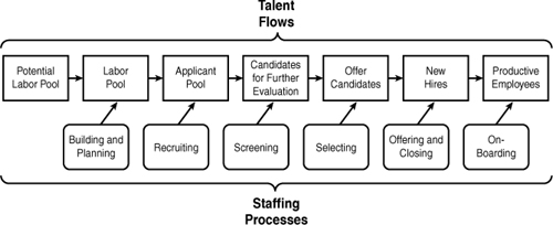
Figure 8-1. Logic of staffing processes and talent flows.

Groups of individuals (talent pools) flow through the various stages of the staffing process, with each stage serving as a filter that eliminates a subset of the original talent pool. The top row of Figure 8-1 shows the results of the filtering process, beginning with a potential labor pool that is winnowed through recruitment and selection to a group that receives offers and then is winnowed further as some accept offers and remain with the organization.

The “staffing processes” in the lower row show the activities that accomplish the filtering sequence, beginning with building and planning (forecasting trends in external and internal labor markets, inducing potential applicants to develop qualifications to satisfy future talent demands), and ending with on-boarding (orientation, mentoring, removing barriers to performance). Integrating measurement categories with the process steps shown in Figure 8-1 provides a decision-based framework for evaluating where staffing measures are sufficient and where they may be lacking.

Figure 8-1 might usefully be viewed as a supply-chain approach to staffing. To appreciate that analogy, consider that the pipeline of talent is very similar to the pipeline of any other resource. At each stage, the candidate pool can be thought of in terms of the quantity of candidates, the average and dispersion of the quality of the candidates, and the cost of processing and employing the candidates. Quantity, quality, and cost considerations determine the monetary value of staffing programs. We have more to say about these ideas in Chapter 10. Now that we have presented the “big picture” of the staffing process, let us focus more specifically on one component of that process: employee selection (specifically, on assessing the value of selection by means of utility analysis).

Our objective in this chapter is to describe three different models of staffing utility analysis, focusing on the logic and analytics of each one. Chapter 9, “The Economic Value of Job Performance,” Chapter 10, and Chapter 11 then build on these ideas, emphasizing measures and processes to communicate results to operating executives and to show how staffing, training, and other HR programs can be evaluated from a return on investment (ROI) perspective.

Similarly, the bottom row of Figure 8-1 reflects the staffing processes that create the sequential filtering of candidates. Each of these processes can be thought of in terms of the quantity of programs and practices used, the quality of the programs and practices as reflected in their ability to improve the value of the pool of individuals that survives, and the cost of the programs and practices in each process. For example, the quality of selection procedures is often expressed in terms of their validity, or accuracy in forecasting future job performance. Validity is typically expressed in terms of the correlation (see Chapter 2) between scores on a selection procedure and some measure of job performance, such as the dollar volume of sales. Validity may be increased by including a greater quantity of assessments (such as a battery of selection procedures), each of which focuses on an aspect of knowledge, skill, ability, or other characteristic that has been demonstrated to be important to successful performance on a job. Higher levels of validity imply higher levels of future job performance among those selected or promoted, thereby improving the overall payoff to the organization. As a result, those candidates who are predicted to perform poorly never get hired or promoted in the first place.

Decision makers naturally focus on the cost of selection procedures because they are so vividly depicted by standard accounting systems, but the cost of errors in selecting, hiring, or promoting the wrong person is often much more important. As explained in Chapter 9, the difference in value between an average performer versus a superior performer is often much higher than the difference in the cost of improving the staffing process. In the case of executives, a company often has to pay large fees to headhunters, and poor performance can have serious consequences in terms of projects, products, and customers. That cost can easily run $1 million to $3 million.⁷

In summary, the overall payoff to the organization (utility) from the use of staffing procedures depends on three broad parameters: quantity, quality, and cost. Each of the three staffing utility models that we examine in this chapter addresses two or more of these parameters. The models usually focus on the selection part of the processes of Figure 8-1, but they have implications for the other staffing stages, too. Each model defines the quality of candidates in a somewhat different way, so we start with the models that make relatively basic assumptions and move to those that are increasingly sophisticated.

• The proportion of individuals in the selected group who are considered successful

• The average standard score on a measure of job performance for the selected group

• The dollar payoff to the organization resulting from the use of a particular selection procedure

The remainder of this chapter considers each of these utility models and its associated measure of quality in greater detail.

Taylor and Russell defined the value of the selection system as the “success ratio,” which is the ratio of the number of hired candidates who are judged successful on the job divided by the total number of candidates that were hired. They published a series of tables illustrating the interactive effect of different validity coefficients, selection ratios, and base rates on the success ratio. The success ratio indicates the quality of those selected. The difference between the success ratio and the base rate (which reflects the success ratio without any added selection system) is a measure of the incremental value of the selection system over what would have happened if it had not been used. Let’s develop this logic and its implications in more detail and show you how to use the tables Taylor and Russell developed.

Analytics

This model has three key, underlying assumptions:

1. It assumes fixed-treatment selection. (That is, individuals are chosen for one specified job, treatment, or course of action that cannot be modified.) For example, if a person is selected for Treatment A, a training program for slow learners, transfer to Treatment B, fast-track instruction, is not done, regardless of how well the person does in Treatment A.
2. The Taylor-Russell model does not account for the rejected individuals who would have been successful if hired (erroneous rejections). Because they are not hired, their potential value, or what they might contribute to other employers who now can hire them, is not considered.
3. The model classifies accepted individuals into successful and unsuccessful groups. All individuals within each group are regarded as making equal contributions. That means that being minimally successful is assumed to be equal in value to being highly successful, and being just below the acceptable standard is assumed to be equal in value to being extremely unsuccessful.

Of course, these assumptions may not hold in all situations; but even with these basic assumptions, Taylor and Russell were able to generate useful conclusions about the interplay between testing and recruitment. For example, the Taylor-Russell model demonstrates convincingly that even selection procedures with relatively low validities can increase substantially the percentage of those selected who are successful, when the selection ratio is low (lots of candidates to choose from) and when the base rate is near 50 percent (about half the candidates would succeed without further testing, so there are lots of middle-level candidates who can be sorted by better selection). Let us consider the concepts of selection ratio and base rate in greater detail.

The selection ratio is simply the number of candidates who must be hired divided by the number of available candidates to choose from. A selection ratio (SR) of 1.0 means the organization must hire everyone, so testing is of no value because there are no selection decisions to be made. The closer the actual SR is to 1.0, the harder it is for better selection to pay off. The opposite also holds true; as the SR gets smaller, the value of better selection gets higher. (For example, a selection ratio of .10 means the organization has ten times more applicants than it needs and must hire only 10 percent of the available applicants.) Figure 8-2 illustrates the wide-ranging effect that the SR may exert on a predictor with a given validity. In each case, Xc represents a cutoff score on the predictor. As you can see in Figure 8-2, even predictors with low validities can be useful if the SR is so low that the organization needs to choose only the cream of the crop. Conversely, with high selection ratios, a predictor must possess very high validity to increase the percentage successful among those selected.

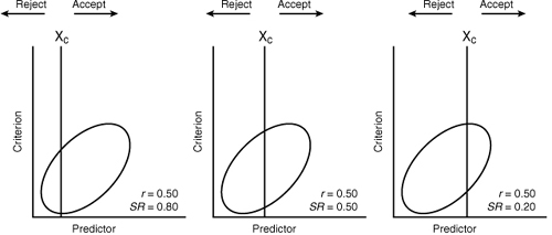
Figure 8-2. Effect of varying selection ratios on a predictor with a given validity.

Note: The oval is the shape of a scatterplot corresponding to r = 0.50; r = validity coefficient; SR = selection ratio; X_c = cutoff score.

It might appear that, because a predictor that demonstrates a particular validity is more valuable with a lower selection ratio, one should always opt to reduce the SR (become more selective). However, the optimal strategy is not this simple.¹² When the organization must achieve a certain quota of individuals, lowering the SR means the organization must increase the number of available applicants, which means expanding the recruiting and selection effort. In practice, that strategy may be too costly to implement, as later research demonstrated convincingly.¹³

Utility, according to Taylor and Russell, is affected by the base rate (the proportion of candidates who would be successful without the selection measure). To be of any use in selection, the measure must demonstrate incremental validity by improving on the BR. That is, the selection measure must result in more correct decisions than could be made without using it. As Figure 8-3 demonstrates, when the BR is either very high or very low, it is difficult it for a selection measure to improve upon it.

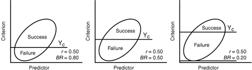
Figure 8-3. Effect of varying base rates on a predictor with a given validity.

Note: The oval is the shape of a scatterplot corresponding to r = 0.50; BR = base rate; r = validity coefficient; Y_c = minimum level of job performance.

In each panel of the figure, Y_c represents the minimum level of job performance (criterion cutoff score) necessary for success. That value should not be altered arbitrarily. Instead, it should be based on careful consideration of the true level of minimally acceptable performance for the job.¹⁴ Figure 8-3 illustrates that, with a BR of 0.80, it would be difficult for any selection measure to improve on the base rate. In fact, when the BR is 0.80 and half of the applicants are selected, a validity of 0.45 is required to produce an improvement of even 10 percent over base-rate prediction. This is also true at very low BRs (as would be the case, for example, in the psychiatric screening of job applicants). Given a BR of 0.20, an SR of 0.50, and a validity of 0.45, the percentage successful among those selected is 0.30 (once again representing only a 10 percent improvement in correct decisions). Selection measures are most useful when BRs are about 0.50.¹⁵ Because the BR departs radically in either direction from this value, the benefit of an additional predictor becomes questionable. The lesson is obvious: Applications of selection measures to situations with markedly different SRs or BRs can result in quite different predictive outcomes. If it is not possible to demonstrate significant incremental utility by adding a predictor, the predictor should not be used, because it cannot improve on current selection procedures.

Figure 8-4 presents all of the elements of the Taylor-Russell model together. In this figure, the criterion cutoff (Y_c) separates the present employee group into satisfactory and unsatisfactory workers. The predictor cutoff (X_c) defines the relative proportion of workers who would be hired at a given level of selectivity. Areas A and C represent correct decisions—that is, if the selection measure were used to select applicants, those in area A would be hired and become satisfactory employees. Those in area C would be rejected correctly because they scored below the predictor cutoff and would have performed unsatisfactorily on the job. Areas B and D represent erroneous decisions; those in area B would be hired because they scored above the predictor cutoff, but they would perform unsatisfactorily on the job, and those in area D would be rejected because they scored below the predictor cutoff, but they would have been successful if hired.

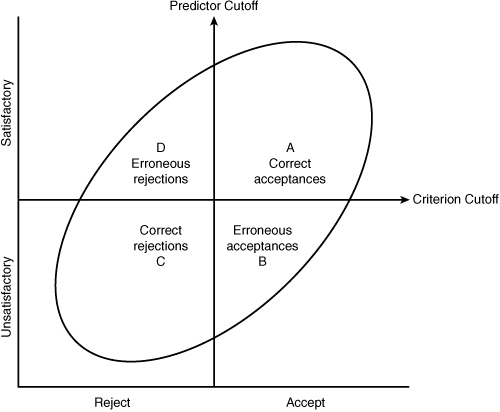
Figure 8-4. Effect of predictor and criterion cutoffs on selection decisions.

Note: The oval is the shape of the scatterplot that shows the overall relationship between predictor and criterion scores.

Taylor and Russell used the following ratios in developing their tables:

8-1.

8-2.

8-3.

By specifying the validity coefficient, the base rate, and the selection ratio, and making use of Pearson’s “Tables for Finding the Volumes of the Normal Bivariate Surface,”¹⁶ Taylor and Russell developed their tables (see Appendix A). The usefulness of a selection measure thus can be assessed in terms of the success ratio that will be obtained if the selection measure is used. To determine the gain in utility to be expected from using the instrument (the expected increase in the percentage of successful workers), subtract the base rate from the success ratio (Equation 8-3 minus Equation 8-1). For example, given an SR of 0.10, a validity of 0.30, and a BR of 0.50, the success ratio jumps to 0.71 (a 21 percent gain in utility over the base rate—to verify this figure, see Appendix A).

The validity coefficient referred to by Taylor and Russell is, in theory, based on present employees who have already been screened using methods other than the new selection procedure. It is assumed that the new procedure will simply be added to a group of selection procedures used previously, and the incremental gain in validity from the use of the new procedure most relevant.

Perhaps the major shortcoming of this utility model is that it reflects the quality of the resulting hires only in terms of success or failure. It views the value of hired employees as a dichotomous classification—successful or unsuccessful—and as the tables in Appendix A demonstrate, when validity is fixed, the success ratio increases as the selection ratio decreases. (Turn to Appendix A, choose any particular validity value, and note what happens to the success ratio as the selection ratio changes from 0.95 to 0.05.) Under those circumstances, the success ratio tells us that more people are successful, but not how much more successful.

In practice, situations may arise in which one would not expect the average level of job performance to change as a function of higher selection standards, such as food servers at fast-food restaurants. Their activities have become so standardized that there is little opportunity for significant improvements in performance after they have been selected and trained. The relationship between the value of such jobs to the organization and variations in performance demonstrates essentially flat slopes. In such situations, it may make sense to think of the value of hired candidates as either being above the minimum standard or not.

For many jobs, however, one would expect to see improvements in the average level of employee value from increased selectivity. In most jobs, for example, a very high-quality employee is more valuable than one who just meets the minimum standard of acceptability. When it is reasonable to assume that the use of higher cutoff scores on a selection device will lead to higher levels of average job performance by those selected, the Taylor-Russell tables underestimate the actual amount of value from the selection system. That observation led to the development of the next framework for selection utility, the Naylor-Shine Model.

Like Taylor and Russell, Naylor and Shine assume that the relationship between predictor and criterion is bivariate normal (both scores on the selection device and performance scores are normally distributed), linear, and homoscedastic. The validity coefficient is assumed to be based on the concurrent validity model.¹⁸ That model reflects the gain in validity from using the new selection procedure over and above what is presently available using current information.

In contrast to the Taylor-Russell utility model, the Naylor-Shine approach assumes a linear relationship between validity and utility. That is, the higher the validity, the greater the increase in the average criterion score of the selected group compared to the average criterion score that the candidate group would have achieved. Equation 8-4 shows the basic equation underlying the Naylor-Shine model:

8-4.

Here, is the average criterion score (in standard-score units)¹⁹ of those selected, r_xy is the validity coefficient, λ_i is the height of the normal curve at the predictor cutoff, Z_xi (expressed in standard-score units), and φ_i is the selection ratio. Equation 8-4 applies whether r_xy represents a correlation between two variables or it is a multiple-regression coefficient.²⁰

Using Equation 8-4 as a basic building block, Naylor and Shine present a series of tables (see Appendix B) that specify, for each SR, the standard (predictor) score that produces that SR, the ordinate of the normal curve at that point, and the quotient λ_i/φ_i. The quotient , the average predictor score of those selected. The tables can be used to answer several important HR questions:

• Given a specified SR, what will be the average criterion level (for example, performance level) of those selected?

• Given a certain minimum cutoff score on the selection device above which everyone will be hired, what will be the average criterion level ()?

• Given a desired improvement in the average criterion score (for example, performance) of those selected, and assuming a certain validity, what SR and/or predictor cutoff value (in standard score units) should be used?

Let’s work through some examples, using the tables in Appendix B.

In each of the following examples, assume that r_xy, the validity of our predictor, is positive and equal to 0.40. Of course, it is also possible that the validity of a predictor could be negative (for example, higher levels of job satisfaction related systematically to lower intentions to quit). Under these circumstances, the general rule is to reverse the sign of r_xy and Z_xi everywhere in the calculations.

1. With a selection ratio of 50 percent (φ_i = 0.50), what will be the average performance level of those selected?
   

   Solution: Enter the table at φ_i = 0.50 and read λ_i/φ_i = 0.80.

   

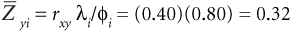
   Thus, the average criterion score of those selected, using an SR of 0.50, is 0.32 Z-units (roughly one third of a standard deviation) better than the unselected sample.

2. With a desired cutoff score set at .96 standard deviations below the average of the applicant pool (Z_xi = –0.96), what will be the standardized value of the criterion ()?
   

   Solution: Enter the table at Z_xi = –0.96 and read λ_i/φ_i = 0.30.

   

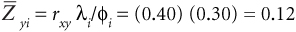
   Thus, using this cutoff score on our predictor results in an average criterion score of about one eighth of a standard deviation (0.12 Z-units) higher than the average of the unselected applicant pool.

3. If we want to achieve an average standardized level of performance on our criterion (such as job performance) among those selected that is half a standard deviation higher than the average of the applicant pool(), and assuming a validity of .40, what SR do we need to achieve? What predictor cutoff value will achieve that SR?
   

   Solution: Because 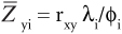then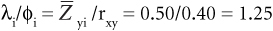

   

   Enter the table at λ_i/φ_i = 1.25 and read φ_i = 0.2578 and Z_xi = 0.65. Thus, to achieve an average improvement of 0.50 (one half) standard deviation in job performance, an SR of 0.2578 is necessary (we must select only the top 25.78 percent of applicants). To achieve that, we must set a cutoff score on the predictor of 0.65 standard deviations above the average among our applicants.

   The Naylor-Shine utility approach is more generally applicable than Taylor-Russell because, in many, if not most, cases, an organization could expect an increase in average job performance as it becomes more selective, using valid selection procedures. However, “average job performance” is expressed in terms of standard (Z) scores, which are more difficult to interpret than are outcomes more closely related to the specific nature of a business, such as dollar volume of sales, units produced or sold, or costs reduced. With only a standardized criterion scale, one must ask questions such as “Is it worth spending $10,000 to select 50 people per year, to obtain a criterion level of 0.50 standard deviations (SDs) greater than what we would obtain without the predictor?”²¹ Some HR managers may not even be familiar with the concept of a standard deviation and would find it difficult to attach a dollar value to a 0.50 SD increase in criterion performance.

   Neither the Taylor-Russell nor the Naylor-Shine models formally integrates the concept of selection system cost, nor the monetary gain or loss, into the utility index. Both describe differences in the percentage of successful employees (Taylor-Russell) or increases in average criterion score (Naylor-Shine), but they tell us little about the benefits to the employer in monetary terms. The Brogden-Cronbach-Gleser model, discussed next, was designed to address these issues.

Brogden showed that, under certain conditions, the validity coefficient is a direct index of “selective efficiency.” That means that if the criterion and predictor are expressed in standard score units, r_xy represents the ratio of the average criterion score made by persons selected on the basis of their predictor scores () to the average score made if one had selected them based on their criterion scores (,). Of course, it is usually not possible to select applicants based on their criterion scores (because one cannot observe their criterion scores before they are hired), but Brogden’s insight means that the validity coefficient represents the ratio of how well an actual selection process does, compared to that best standard. Equation 8-5 shows this algebraically:

8-5.

The validity coefficient has these properties when (1) both the predictor and criterion are continuous (that is, they can assume any value within a certain range and are not divided into two or more categories), (2) the predictor and criterion distributions are identical (not necessarily normal, but identical), (3) the regression of the criterion on the predictor is linear, and (4) the selection ratio (SR) is held constant.²²

As an illustration, suppose that a firm wants to hire 20 people for a certain job and must choose the best 20 from 85 applicants. Ideally, the firm would hire all 85 for a period of time, collect job performance (criterion) data, and retain the best 20, those obtaining the highest criterion scores. The average criterion score of the 20 selected this way would obviously be the highest obtainable with any possible combination of 20 of the 85 applicants.

Such a procedure is usually out of the question, so organizations use a selection process and choose the 20 highest scorers. Equation 8-5 indicates that the validity coefficient may be interpreted as the ratio of the average criterion performance of the 20 people selected on the basis of their predictor scores compared to the average performance of the 20 who would have been selected had the criterion itself been used as the basis for selection. To put a monetary value on this, if selecting applicants based on their actual behavior on the job, would save an organization $300,000 per year over random selection, a selection device with a validity of 0.50 could be expected to save $150,000 per year. Utility is therefore a direct linear function of validity, when the conditions noted previously are met.

Equation 8-5 does not include the cost of selection, but Brogden later used the principles of linear regression to demonstrate the relationships of cost of selection, validity, and selection ratio to utility, expressed in terms of dollars.²³

Recall that our ultimate goal is to identify the monetary payoff to the organization when it uses a selection system to hire employees. To do this, let’s assume we could construct a criterion measure expressed in monetary terms. We’ll symbolize it as y_$. Examples of this might include the sales made during a week/month/quarter by each of the salespersons on a certain job, or the profit obtained from each retail operation managed by each of the store managers across a country, or the outstanding customer debts paid during a week/month/quarter for the customers handled by each of a group of call-center collection agents. If we call that criterion measure y, then here is a plain-English and mathematical description of Brogden’s approach.²⁴

Step 1: Express the Predictor-Criterion Relationship As a Formula for a Straight Line

Recall the formula for a straight line that most people learn in their first algebra class, shown here as Equation 8-6.

8-6.

where:

y = dependent variable, or criterion (such as a job performance measure)

x = independent variable that we hope predicts our criterion (such as job performance)

a = y-intercept, or where the line crosses the y-axis of a graph when x = 0

b = slope, or “rise over the run” of the line—that is, the change in y (for example, change in sales) for every one-unit change in x (score on a sales-aptitude test).

First, let’s change this equation slightly. Let’s substitute the symbol b₀ for a, b₁ for b, and y_$ for y. In this way, we go from Equation 8-6 above to Equation 8-7.

8-7.

Then let’s add an e after the x, to reflect that there is some random fluctuation or “error” in any straight-line estimate, and we get Equation 8-8.

8-8.

Our original formulas (Equations 8-6 and 8-7) described the points that fall exactly on a straight line, but Equation 8-8 describes points that fall around a straight line. Figure 8-5 shows this idea as a straight line passing through an ellipse. The ellipse represents the cloud of score combinations that might occur in an actual group of people, and the line in the middle is the one that gets as close as possible to as many of the points in the cloud. Some people describe this picture as a hot dog on a stick.

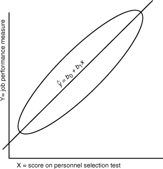
Figure 8-5. Dispersion of actual criterion and predictor scores.

In the context of staffing, x would be each employee’s score on some selection process, and y would be the same employee’s subsequent criterion score (such as performance on the job). If we don’t know yet how someone is going to perform on the job (which we can’t know before the person is hired), a best guess or estimate of how the employee might perform on the job would be the ŷ_$ value obtained from plugging the applicant’s x score into Equation 8-7.

The letter e in Equation 8-8 is called “error,” because although our estimate ŷ_$ from Equation 8-7 might be a good guess, it is not likely to be exactly the level of job performance obtained by that applicant later on the job. Note that because y is the actual performance attained by that applicant, then y – ŷ_$ = e. The “error” by which our original predicted level of job performance, ŷ_$, differed from the applicant’s actual job performance, y, is equal to e.

Ordinary least-squares regression analyses can be used to calculate the “best”-fitting straight line (that is, Equation 8-7), where best means the formula for the straight line ŷ_$ = b₀ + b₁x (Equation 8-7) that minimizes the sum of all squared errors (e²). This is where the “least-squares” portion of the “ordinary least-squares” label comes from.

Step 2: Standardize x

To get back to the validity coefficient, we need to convert the actual, or “raw,” scores on our predictor and criterion to standardized form. Starting with Equation 8-7, reprinted here as Equation 8-9, let’s see how this works.

8-9.

Let’s first standardize all the applicants’ selection process scores (that is, take their original scores, subtract the average, and divide by the standard deviation), as shown in Equation 8-10:

8-10.

Where:

x_i = selection process score earned by applicant i

z_i = “standard” or Z score corresponding to the x_i score for applicant i

= average or mean selection process score, typically of all applicants, obtained in some sample

SD_x = standard deviation of xi around , or

When Equation 8-9 is modified to reflect the fact that x is now standardized, it becomes Equation 8-11.

8-11.

Step 3: Express the Equations in Terms of the Validity Coefficient

Finally, let’s modify Equation 8-11 to show the role of the validity coefficient using this selection process. We want to know the expected value (or the most likely average value) of y_$ for the hired applicants. Modifying Equation 8-11 to express all the elements with a capital E for expected value, we have this:

8-12.

Thus, E(y_$) means the “expected value of the criterion, y, in monetary terms.” Also note that the letter s is now subscripted to the letter z, to show that the criterion scores are from the group of applicants who are actually selected (subscript s stands for “selected”).

Remember that “expected value” typically means “average,” so E(y_$) = _s and . Substituting these values into Equation 8-11 yields the following:

8-13.

We can calculate simply by standardizing the selection test scores of all applicants, averaging just the scores of the individuals who were actually selected (hence the subscript s). When no selection system is used (that is, if applicants had been chosen at random), zs is expected to be the same as the average of z scores for all applicants. By definition, the average of all z scores in a sample is always 0. So when . then also, and E(b₀) will be the average monetary value of the criterion for individuals selected at random from the applicant pool. The symbol for the expected or average monetary criterion score for all applicants is $, so we can substitute $ for E(b₀) in Equation 8-13.

Finally, the value of E(b₁) is obtained using multiple-regression software (for example, the regression function in Excel). This is the regression coefficient or beta weight associated with x (as opposed to the “constant,” which is the estimate of E(b₀)). By definition, the regression coefficient can also be defined as in Equation 8-14.

8-14.

where:

r_xy = simple correlation between test scores on the personnel selection test x and the criterion measure y.

SD_y = standard deviation of the monetary value of the criterion (such as job performance).

SD_x = standard deviation of all applicants’ selection-test scores.

Recall, however, that we standardized applicant test scores in using Equation 8-10 to create the z variable used in Equation 8-11. The standard deviation of z scores is always 1.0. So substituting 1 for SD_x, Equation 8-14 becomes b₁ = r_xySD_y.

Substituting μ_$ for E(b₀) and r_xySD_y for b₁ in Equation 8-13, we get this:

8-15.

Equation 8-15 describes the total expected monetary value of each selected applicant. To calculate the expected average improvement in utility, or the improvement in the monetary value produced by using the staffing system, we can subtract the expected value without using the system, which is μ_$, from both sides of equation. Because μ_$ is the monetary value of criterion performance the organization expects when it chooses applicants at random, _$ – μ_$ is equal to the expected gain in monetary-valued performance from using the staffing process, as shown in Equation 8-16.

8-16.

Step 4: Subtract the Costs of the Selection Process

Selecting applicants requires resources. If we use the letter C to stand for the cost of applying the selection process to one applicant, and the term N_a to stand for the total number of applicants to whom the selection process is applied, then the total cost of the selection process is the product of N_a and C. If we divide that by the number of applicants actually selected, that gives us the average cost of the selection process per selected applicant. Finally, if we subtract the average selection process cost per selected applicant from the average value expressed in Equation 8-15, we get Equation 8-17.

8-17.

Finally, the left side of Equation 8-17 is often symbolized as ΔU, to stand for the “change in utility” per applicant selected, as shown in Equation 8-18.

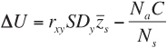
8-18.

Cronbach and Gleser elaborated and refined Brogden’s derivations with respect to utility in fixed-treatment selection, and they arrived at the same conclusions regarding the effects of r, SDy, the cost of selection, and the selection ratio on utility in fixed-treatment selection. Utility properly is regarded as linearly related to validity and, if cost is zero, is proportional to validity.²⁵ They also adopted Taylor and Russell’s interpretation of the validity coefficient for utility calculations (that is, concurrent validity). The validity coefficient based on present employees assumes a population that has been screened using information other than the new selection measure. The selection ratio is applied to this population.

Cronbach and Gleser argued, as did Taylor and Russell and Naylor and Shine, that selection procedures should be judged on the basis of their contribution over and above the best strategy available that makes use of prior, existing information. Thus, any new procedure must demonstrate incremental utility before it is used. Suppose, however, that an organization wants to replace its old selection procedures with new ones. Under such circumstances, the appropriate population for deriving a validity coefficient, SD_y, and SR, should be the unscreened population.²⁶ Figure 8-6 presents a summary of the three utility models that we have discussed.

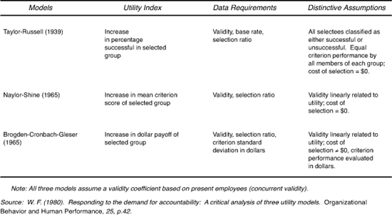
Table 8-6. Summary of the utility indexes, data requirements, and assumptions of three utility models.

To do that, we believe there is much to learn from the field of supply-chain analysis. Supply-chain analysis pays careful attention to the ultimate quality of materials and components. Reframing utility analysis within that framework makes optimization opportunities more apparent. Perhaps more important, the supply-chain framework may help solve one of the thorniest issues in utility analysis: the disturbingly stubborn difficulty in getting key decision makers to embrace it. How? By relating utility analysis to a framework that is familiar to decision makers outside of HR, and one that they already use.

Essentially, the decision process involves optimizing costs against price and time, to achieve levels of expected quality/quantity and risks associated with variations in quality/quantity. If the quality or quantity of acquired resources falls below standard or exhibits excessive variation, decision makers can evaluate where investments in the process will make the biggest difference.

When a line leader complains that he or she is getting inferior talent, or not enough talent for a vital position, HR too often devises a solution without full insight into the broader supply chain. HR often responds by enhancing interviews or tests and presenting evidence about the improved validity of the selection process. Yet a more effective solution might be to retain the original selection process with the same validity, but to recruit from sources where the average quality of talent is higher.

Likewise, consider what happens when business leaders end up with too few candidates, and instruct HR to widen the recruitment search. HR is often too eager to respond with more recruiting activities, when, in fact, the number of candidates presented to business leaders is already sufficient. The problem is that some leaders are better at inducing candidates to accept offers. The more prudent response may be to improve the performance of the leaders who cause candidates to reject offers.

Leaders are accustomed to a logical approach that optimizes all stages of the supply chain when it comes to raw materials, unfinished goods, and technology. Why not adopt the same approach to talent? Consider an example of one company that did just that.

Valero Energy, the 20,000-employee, $70 billion energy-refining and marketing company, developed a new recruitment model out of human capital metrics based on applying supply-chain logic to labor. According to Dan Hilbert, Valero’s manager of employment services, “Once you run talent acquisition as a supply chain, it allows you to use certain metrics that you couldn’t use in a staffing function .... We measure every single source of labor by speed, cost, and efficiency.”²⁸ Computer-screen “dashboards” show how components in the labor supply chain, such as ads placed on online job boards, are performing according to those criteria. If the dashboard shows “green,” performance is fine. If it shows “yellow” or “red,” Valero staffing managers can intervene quickly to fix the problem.²⁹ By doing that, the company can identify where it can recruit the best talent at the most affordable price. From a strategic perspective, it also can identify whether it is better to recruit full-time or part-time, to contract workers, or to outsource the work entirely.

We have more to say in later chapters about applying supply-chain logic to decisions about talent, but for now, the important point to emphasize is that talent flows and staffing processes are parts of a larger system. Our objective should be to optimize overall decisions regarding quantity, quality, and cost against price and time.

This chapter presents some complex but elegant statistical logic. It’s sometimes hard to follow at first, but as Figure 8-1 shows, it is actually rather intuitive. The idea of each of the three “selection utility” models is to estimate how much higher the quality of the selected employees will be, compared to the quality of the candidates for selection. That change in quality depends on how selective the organization can be, how well it predicts future performance, and how much differences in performance quality translate into differences in value to the organization.

The utility models are best used with an understanding of their logic, assumptions, and data requirements. If you make that investment, you have a logical system for making wiser and more strategically relevant decisions about how to select talent both from the outside and within the organization.

These equations would be fine if we actually had a monetarily valued criterion to use in estimating SD_y. When a job produces very clear monetarily valued outcomes such as sales, waste, or profit, we might associate these values with each individual on the job and calculate the standard deviation of those values. Still, that would not reflect the standard deviation we might have seen in the pool of applicants, because the people on the job have already been screened in the course of the selection process. Also, even in jobs with obvious monetary outcomes, such as sales, other elements of the job may be quite important but are not reflected in individual monetary results (such as when salespeople actually sell less because they are training their colleagues). In short, the value and the process for estimating SD_y address a fundamental question in all of human resources and talent management: “How much are differences in performance worth?”

At this point, you might be wondering how organizations can actually estimate the dollar value of differences in performance quality. Indeed, SD_y has been the subject of much debate, and there are several methods for estimating it. We discuss those in the next chapter. You might also wonder whether this same kind of logic (estimating how much better quality our employees are after a certain HR program, compared to their quality without it) might apply to programs other than selection. We have much more to say about the strategic use of utility analysis in guiding investment decisions about human capital in Chapters 10 and 11.

1. Use the Taylor-Russell tables (see Appendix A) to solve these problems by filling in the following table:
   
   
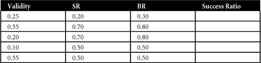
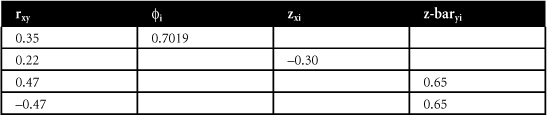
2. Use the Naylor-Shine tables (see Appendix B) to solve these problems by filling in the following table:
   
   
3. Using the Brogden-Cronbach-Gleser continuous-variable utility model, what is the net gain over random selection (ΔU overall and per selectee), given the following information?
   

   Quota for selection: 20

   SR: 0.20

   SD_y (standard deviation of job performance expressed in dollars): $30,000

   r_xy: 0.25

   C_y: $35

   Hint: To find N, the number recruited, divide the quota for selection by the SR.

4. Given the following information on two selection procedures, and using the Brogden-Cronbach-Gleser model, what is the relative difference in payoff (overall and per selectee) between the two procedures? For both procedures, quota = 50, SR = 0.50, and SD_y = $45,000.
   

   r_y1: 0.20 c₁: $200

   r_y2: 0.40 c₂: $700

5. You are a management consultant whose task is to do a utility analysis using the following information regarding secretaries at Inko, Inc. The validity of the Secretarial Aptitude Test (SAT) is 0.40, applicants must score 70 or better to be hired, and only about half of those who apply actually are hired. Of those hired, about half are considered satisfactory by their bosses. How selective should Inko be to upgrade the average criterion score of those selected by What utility model did you use to solve the problem? Why?

2. Cascio, W. F., and L. Fogli, “The Business Value of Employee Selection,” in Handbook of Employee Selection, ed. J. L. Farr and N. T. Tippins (pp. 235–252). (New York: Routledge, 2010).

3. Ibid. See also Boudreau, J. W., and P.M. Ramstad, “Beyond Cost-Per-Hire and Time to Fill: Supply-Chain Measurement for Staffing,” Los Angeles, CA: Center for Effective Organizations, CEO publication G 04-16 (468).

4. Boudreau, J. W., and P.M. Ramstad, “Strategic Industrial and Organizational Psychology and the Role of Utility Analysis Models,” in Handbook of Psychology 12, ed. W. C. Borman, D. R. Ilgen, and R. J. Klimoski, (pp. 193-221). (Hoboken, N.J.: Wiley, 2003).

5. Brealey, R. A., S. C. Myers, and F. Allen, Principles of Corporate Finance, 8th ed. (Burr Ridge, Ill.: Irwin/McGraw-Hill, 2006).

6. Cronbach, L. J., and G. C. Gleser, Psychological Tests and Personnel Decisions, 2nd ed. (Urbana, Ill.: University of Illinois Press, 1965).

7. Byrnes, N., and D. Kiley, “Hello, You Must Be Going,” BusinessWeek, February 12, 2007, 30–32; and Berner, R., “My Year at Wal-Mart,” BusinessWeek, February 12, 2007, 70–74.

8. Blum, M. L., and J. C. Naylor, Industrial Psychology: Its Theoretical and Social Foundations, revised ed. (New York: Harper & Row, 1968).

9. Taylor, H. C., and J. T. Russell, “The Relationship of Validity Coefficients to the Practical Effectiveness of Tests in Selection,” Journal of Applied Psychology 23 (1939): 565–578.

10. Naylor, J. C., and L. C. Shine, “A Table for Determining the Increase in Mean Criterion Score Obtained by Using a Selection Device,” Journal of Industrial Psychology 3 (1965): 33–42.

11. Brogden, H. E., “On the Interpretation of the Correlation Coefficient As a Measure of Predictive Efficiency,” Journal of Educational Psychology 37 (1946): 64–76; Brogden, H. E., “When Testing Pays Off,” Personnel Psychology 2 (1949): 171–185; and Cronbach and Gleser, 1965.

12. Sands, W. A., “A Method for Evaluating Alternative Recruiting-Selection Strategies: The CAPER Model,” Journal of Applied Psychology 57 (1973): 222–227.

13. Boudreau, J. W., and S. L. Rynes, “Role of Recruitment in Staffing Utility Analyses,” Journal of Applied Psychology 70 (1985): 354–366.

14. Boudreau, J. W., “Utility Analysis for Decisions in Human Resource Management,” in Handbook of Industrial and Organizational Psychology 2 (2nd ed.), ed. M. D. Dunnette and L. M. Hough (Palo Alto, Calif.: CPP, 1991).

15. Taylor and Russell, 1939.

16. Pearson, K., Tables for Statisticians and Biometricians, vol. 2 (London: Biometric Laboratory, University College, 1931).

17. Naylor and Shine, 1965.

18. This means that the new selection procedure is administered to present employees who already have been screened using other methods. The correlation (validity coefficient) between scores on the new procedure and the employees’ job performance scores is then computed.

19. To transform raw scores into standard scores, we used the following formula : x – ÷ SD, where x is the raw score, is the mean of the distribution of raw scores, and SD is the standard deviation of that distribution. Assuming that the raw scores are distributed normally, about 99 percent of the standard scores will lie within the range –3 to + 3. Standard scores (Z-scores) are expressed in standard deviation units.

20. A multiple-regression coefficient represents the correlation between a criterion and two or more predictors.

21. Boudreau, 1991.

22. Brogden, 1946.

23. Brogden, 1949.

24. The authors would like to thank Professor Craig J. Russell for allowing us to adapt the framework that he developed.

25. Cronbach and Gleser, 1965.

26. Boudreau, 1991.

27. Material in this section comes from Cascio, W. F., and J. W. Boudreau, “Utility of Selection Systems: Supply-Chain Analysis Applied to Staffing Decisions,” in Handbook of I/O Psychology, Vol. 2, ed. S. Zedeck (Washington, D.C.: American Psychological Association, 2011, pp. 421-444).

28. Hilbert, cited in Schneider, C., “The New Human-Capital Metrics,” retrieved August 5, 2008 from www.cfo.com.

29. Valero Energy, “2006 Optimas Awards,” Workforce Management (March 13, 2006).

References

1. Crainer, S., and D. Dearlove, “Whatever Happened to Yesterday’s Bright Ideas?” Across the Board (May/June 2006): 34–40.