Chapter 9. The Economic Value of Job Performance

Consider this single question: Where would a change in the availability or quality of talent have the greatest impact on the success of your organization? Talent pools that have great impact are known as pivotal talent pools. Alan Eustace, Google’s vice president of engineering, told The Wall Street Journal that one top-notch engineer is worth 300 times or more than the average and that he would rather lose an entire incoming class of engineering graduates than one exceptional technologist.¹

This estimate was probably not based on precise numbers, but the insight it reveals regarding where Google puts its emphasis is significant. Recasting performance management to reflect where differences in performance have large impact allows leaders to engage the logic they use for other resources and make educated guesses that can be informative.² In defining pivotal talent, an important distinction is often overlooked. That distinction is between average value and variability in value. When strategy writers describe critical jobs or roles, they typically emphasize the average level of value (for example, the general importance, customer contact, uniqueness, or power of certain jobs). Yet a key question for managers is not which talent has the greatest average value, but rather, in which talent pools performance variation creates the biggest strategic impact.³

Impact (discussed in Chapter 1, “Making HR Measurement Strategic”) identifies the relationship between improvements in organization and talent performance, and sustainable strategic success. The pivot point is where differences in performance most affect success. Identifying pivot points often requires digging deeply into organization- or unit-level strategies to unearth specific details about where and how the organization plans to compete, and about the supporting elements that will be most vital to achieving that competitive position. These insights identify the areas of organization and talent that make the biggest difference in the strategy’s success.⁴

Consider a Disney theme park. Suppose we ask the question the usual way: What is the important talent for theme park success? What would you say? There’s always a variety of answers, and they always include the characters. Indeed, characters such as the talented people inside the Mickey Mouse costumes are very important. The question of talent impact, however, focuses on pivot points. Consider what happens when we frame the question differently, in terms of impact: Where would an improvement in the quality of talent and organization make the biggest difference in our strategic success? Answering that question requires looking further to find the strategy pivot points that illuminate the talent and organization pivot points.

One way to find the pivot points in processes is to look for constraints. These are like bottlenecks in a pipeline: If you relieve a constraint, the entire process works better. For a Disney theme park, a key constraint is the number of minutes a guest spends in the park. Disney must maximize the number of “delightful” minutes. Disneyland has 85 acres of public areas, many different “lands,” and hundreds of small and large attractions. Helping guests navigate, even delighting them as they navigate, defines how Disney deals with this constraint. Notice how the focus on the constraint allows us to see beneath the customer delight strategy and identify a pivotal process that supports it.

Figure 9-1 applies this concept to two talent pools in the Disney theme park: Mickey Mouse and the park sweeper.

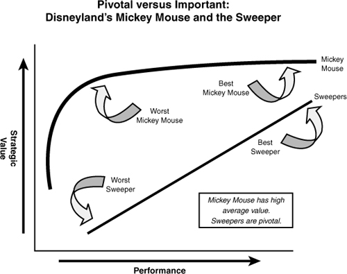
Figure 9-1. Performance-yield curves for sweepers versus Mickey Mouse.

Mickey Mouse is important but not necessarily pivotal. The top line represents the performance of the talent in the Mickey Mouse role. The curve is very high in the diagram because performance by Mickey Mouse is very valuable. However, the variation in value between the best-performing Mickey Mouse and the worst-performing Mickey Mouse is not that large. In the extreme left side of the figure, if the person in the Mickey Mouse costume engaged in harmful customer interactions, the consequences would be strategically devastating. That is shown by the very steep downward slope at the left. That’s why the Mickey Mouse role has been engineered to make such errors virtually impossible. The person in the Mickey Mouse costume is never seen, never talks, and is always accompanied by a supervisor who manages the guest encounters and ensures that Mickey doesn’t fall down, get lost, or take an unauthorized break. What is often overlooked is that because the Mickey Mouse job is so well engineered, there is also little payoff to investing in improving the performance of Mickey Mouse once the person meets the high standards of performance. Mickey should not improvise or take too long with any one guest, because Mickey must follow a precise timetable so that everyone gets a chance to “meet” Mickey and so that guests never see two Mickeys at the same time.

If performance differences that most affect the guest experience are not with Mickey Mouse, then where are they? When a guest has a problem, folks such as park sweepers and store clerks are most likely to be nearby in accessible roles, so guests approach them. People seldom ask Cinderella where to buy a disposable camera, but hundreds a day ask the street sweeper. The lower curve in Figure 9-1 represents sweepers. The sweeper curve has a much steeper slope than Mickey Mouse because variation in sweeper performance creates a greater change in value. Disney sweepers are expected to improvise and make adjustments to the customer service process on-the-fly, reacting to variations in customer demands, unforeseen circumstances, and changes in the customer experience. These make pivotal differences in Disney’s theme park strategy to be the “Happiest Place on Earth.” To be sure, these pivot points are embedded in architecture, creative settings, and the brand of Disney magic. Alignment is key. In fact, it is precisely because of this holistic alignment that interacting with guests in the park is a pivotal role and the sweeper plays a big part in that role. At Disney, sweepers are actually front-line customer representatives with brooms in their hands.⁵

On the other hand, the project leader of an advertising campaign or a salesperson who manages all the accounts in a given territory has considerable discretion in deciding how to accomplish the work. Variation in individual abilities and motivation can lead to large values of SD_y in those jobs, and also relative to other jobs that vary in terms of the autonomy and discretion they permit. Empirical evidence shows that SD_y increases as a function of job complexity.⁷ As jobs become more complex, it becomes more difficult to specify precisely the procedures that should be used to perform them. As a result, differences in ability and motivation become more important determinants of the variability of job performance.

A second factor the influences the size of SD_y is the relative value to the organization of variations in performance. In some jobs, performance differences are vital to the successful achievement of the strategic goals of an organization (for example, software engineers who design new products for leading-edge software companies) and others that are less so (for example, employees who send out bills in an advertising agency). Even though there is variability in performance of employees in the billing department, that variability is not as crucial to the success of the firm as is the variability in the performance of project leaders at the agency. In short, pivotalness—and, thus, SD_y—is affected by the relative position of a job in the value chain of an organization.⁸

In the Disney example shown in Figure 9-1, the sweeper role has a higher SD_y than Mickey Mouse because variations in sweeper performance (particularly when they respond to guests) cause a larger change in strategic value than variations in Mickey Mouse performance. Mickey Mouse is vital to the Disney value chain, however. So it is important to understand the difference between average value of performance and pivotalness, the latter being reflected in SD_y. High pivotalness and high average value often occur together, but not always.

The impact of performance variation in jobs requires considering the strategy of the organization (sustainability, strategic success, pivotal resources and processes, and organization and talent pools).⁹ The same job can have very different implications for performance differences, depending on the strategy and work processes of the organization. Consider the role of front-line associates at two different fast-food organizations: McDonald’s and Starbucks. Both roles involve preparing the product, interacting with customers, taking payments, working with the team, keeping up good attendance, and executing good job performance. The description for these roles might look similar at both Starbucks and McDonald’s, yet McDonald’s and Starbucks choose to compete differently.

McDonald’s is known for consistency and speed. Its stores automate many of the key tasks of food preparation, customer interaction, and team roles. Each McDonald’s product has an assigned number so that associates need only press the number on the register to record the customer order. Indeed, it is not unusual to hear customers themselves ordering by saying, “I’ll take a number 3 with a Coke, and supersize it.” Contrast that with Starbucks. Starbucks baristas are a highly diverse and often multitalented group. The allure of Starbucks as a “third place” (home, work, and Starbucks) is predicated, in part, on the possibility of interesting interactions with Starbucks baristas. Blogs, tweets, and Facebook pages are devoted to the Starbucks baristas. Some of them are opera singers and actually sing out the orders. Their personal styles are clearly on display and range from Gothic to country to hipster. Few online pages are devoted to McDonald’s associates. Starbucks counts on that diversity as part of its image.¹⁰ This means that it needs to give its baristas wide latitude to sing, joke, and chat with customers.

Figure 9-2 shows this relationship graphically, with McDonald’s on the left and Starbucks on the right. McDonald’s designs its systems to limit both the downside of performance mistakes and the upside of too-creative improvising. Starbucks encourages innovation and “style” to get the upside (at the extreme right side is a barista whose style goes “viral,” drawing Internet attention to the brand), accepting the downside on the left (sometimes a barista may do something that offends a few customers).

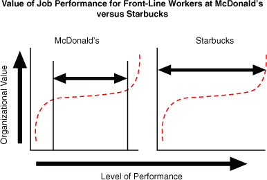
Figure 9-2. Value of job performance for front-line workers at McDonald’s vs. Starbucks.

Graphic depictions of performance-yield curves, such as the ones in Figures 9-1 and 9-2, can help identify where decisions should focus on achieving a minimum standard level of performance (as with billers in an advertising agency or French fries cooks in a fast-food restaurant) versus improving performance (as with sweepers in a theme park or software designers). Such depictions also provide a way to think about the risks and returns to performance at different levels. This helps people avoid making decisions based on well-meaning but potentially simplistic rules, such as “Find the best candidate for every position.”¹¹

Indeed, the idea that performance variation in certain areas has greater impact than performance variation in others is a fundamental premise of engineering, where different components of a product, project, or software program are held to different tolerances, depending on the role they play. The upholstery in a commercial aircraft can vary from its ideal standard by quite a lot, but the hydraulics cannot. This is often called Kano analysis, named after Noriaki Kano, who coined the term in the 1980s. He showed how improved performance has widely differing effects.¹² Thus, approaching work performance in this way allows human resource leaders, I/O psychologists, and business leaders to communicate about work performance using proven business tools, which John Boudreau has termed “retooling HR.”¹³

In terms of measurement, the value of variation in employee performance is an important variable that determines the likely payoff of investments in HR programs. Most HR programs are designed to improve performance. All things equal, such programs have a higher payoff when they are directed at organizational areas where performance variation has a large impact on processes, resources, and, ultimately, strategic success. A 15 percent improvement in performance is not equally valuable everywhere. Ideally, we would like to translate performance improvements into monetary values. If we can do that, we can measure whether the performance improvement we expect from a program, such as more accurate selection, improved training, or more effective recruitment, justifies the cost of the program.

As yet no perfect measure of the value of performance variation exists, but a great deal of research has addressed the issue. We provide a guide to the most important findings in the later sections. First, we show how the value of performance variation (in the form of SD_y) fits into the formulas for the utility, or monetary value, of staffing programs that we discussed in Chapter 8.

Without SD_y, the effect of a change in criterion performance could be expressed only in terms of standard Z-score units. However, when the product, Z-score units are multiplied by the monetary-valued SD_y, the gain is expressed in monetary units, which are more familiar to decision makers. As you will see in Chapter 11, “Costs and Benefits of HR Development Programs,” and in Equation 11-1, the same SD_y variable can also be used to translate the statistical effects of training and development programs into monetary terms.

Note again that we often refer to dollar-valued performance or use the dollar sign as a subscript, but the conclusions are valid for any other currency.

Most parameters of the general utility equation for staffing and for development can be obtained from records. For staffing, this includes such variables as the number of people tested, the cost of testing, and the selection ratio. For development, this includes the number of people trained, the cost of training, and the duration of the training effects. However, SD_y usually cannot be obtained from existing records. Traditionally, SD_y has been the parameter of the utility equation that is the most difficult to obtain.¹⁴ Originally, SD_y was estimated using complicated cost-accounting methods that are both costly and time-consuming. Those procedures involve first costing out the dollar value of the job behaviors of each employee¹⁵ and then computing the standard deviation of these values. The complexity of those approaches led to newer approaches that rely on estimates from knowledgeable persons. The next section describes alternative approaches for measuring SD_y.

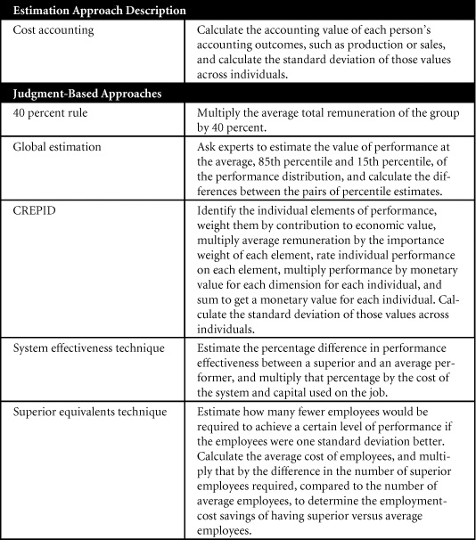
Table 9-1. Alternative Approaches for Estimating SD_y

The remainder of the chapter discusses each of these approaches in more detail.

Cost-accounting estimates of performance value require considering elements such as the following:¹⁶

• Average value of production or service units.

• Quality of objects produced or services accomplished.

• Overhead, including rent, light, heat, cost depreciation, or rental of machines and equipment.

• Errors, accidents, spoilage, wastage, damage to machines or equipment due to unusual wear and tear, and so on.

• Such factors as appearance, friendliness, poise, and general social effectiveness in public relations. (Here, some approximate value would have to be assigned by an individual or individuals having the required responsibility and background.)

• The cost of spent time of other employees and managers. This includes not only the time of supervisors, but also that of other workers.

Researchers in one study attempted to apply these ideas to the job of route salesperson in a Midwestern soft-drink bottling company that manufactures, merchandises, and distributes nationally known products.¹⁷ This job was selected for two reasons: There were many of individuals in the job, and variability in performance levels had a direct impact on output. Route salespersons were paid a small weekly base wage, plus a commission on each case of soft drink sold. The actual cost-accounting method to compute SD_y involved eight steps:

1 Output data on each of the route salespersons was collected from the records of the organization on the number of cases sold and the size and type of package, for a one-year period (to eliminate seasonality).

2 The weighted average sales price per case unit (SP_u) was calculated using data provided by the accounting department.

3 The variable cost per case unit (VC_u) was calculated and subtracted from the average price. Variable costs are costs that vary with the volume of sales, such as direct labor, direct materials (syrup cost, CO2 gas, crowns, closures, and bottles), variable factory overhead (state inspection fees, variable indirect materials, variable indirect labor), and selling expenses (the route salesperson’s commission).

4 Contribution margins per case unit (CM_u) were calculated as the sales price per unit minus the variable cost per unit.

5 The contribution margins calculated in step 4 were multiplied by the output figures (step 1), producing a total one-year dollar-valued contribution margin for each route salesperson. This figure represents the total amount (in dollars and cents) each salesperson contributed toward fixed costs and profit.

6 Not all differences in sales were assumed to be due to differences in route salespersons’ performance. Other factors, such as the type of route, partially determined sales, so it was important to remove these influences. To accomplish this, the sales of each route were partitioned into two categories: home market and cold bottle. Home market represents sales in large supermarkets and chain stores, in which the product is purchased and taken home to consume. Cold bottle represents sales such as those from small convenience stores and vending operations, in which the product is consumed on location. Top management agreed that home market sales are influenced less by the efforts of the route salesperson, but the route salesperson exercises greater influence over the relative sales level in the cold-bottle market because the route salesperson has a greater degree of flexibility in offering price incentives, seeking additional display space, and so forth. The critical question was, “How much influence does the route salesperson have in each of the respective sectors?” The percentage of sales or contributions attributable to the efforts of the route salesperson was determined by a consensus of six top managers, who estimated the portions of home-market sales and cold-bottle sales attributable to the efforts of the route salesperson at 20 percent and 30 percent, respectively.

7 The percentages calculated in step 6 were multiplied by the total contribution margins calculated in step 5, yielding a total contribution margin for each route salesperson. Figure 9-3 shows an example calculation. This served as the cost accounting-based estimate of each route salesperson’s worth to the organization.

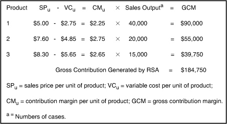
Figure 9-3. Sample of the total contribution attributable to route Salesperson A (RSA) using cost-accounting procedures.

8 The standard deviation of these values was the cost accounting-based estimate of SD_y. This approach, called contribution costing, is generally not used for external reporting purposes, but it is generally recommended for internal, managerial reporting purposes.¹⁸

Cost-accounting systems focus on determining the costs and benefits of units of product, not units of performance, and thus require a good deal of translation to estimate performance value. So although the accounting data on which the estimates are based is often trusted by decision makers, the array of additional estimates required often creates doubt about the objectivity and reliability of the cost-accounting estimates. Over the past few decades, several alternative approaches for estimating the economic value of job performance have been developed that require considerably less effort than the cost-accounting method. Comparative research has made possible some general conclusions about the relative merits of these methods.

To examine whether the standard deviation of output was about 20 percent of average output, a summary of the results of 68 studies that measured work output or work samples found that low-complexity jobs such as routine clerical or blue-collar work had SD_p values that averaged 15 percent of output. Medium-complexity jobs such as first-line supervisors, skilled crafts, and technicians had average SD_p values of 25 percent, and high-complexity jobs, such as managerial/professional, and complex technical jobs had average SD_p values of 46 percent. For life-insurance sales jobs, SD_p was very large (97 percent of average sales), and it was 39 percent for other sales jobs.²² It appears that there are sizable differences in the amounts of performance variation in different jobs (recall how different the performance variation was among sweepers versus Mickey Mouse), and the 20 percent rule may underestimate or overestimate them.

Based on this evidence, some have suggested that SD_p might be directly estimated from the complexity of the job. In other words, use a value of 39 percent for sales jobs, 15 percent for clerical jobs, and so on. A drawback is that SD_p is expressed as the percentage of average output, not in monetary values.²³ Getting a monetary value thus would require multiplying the percentage by the money value of average output. You could try to estimate the monetary value of average output in a job, but that has many of the same difficulties as the cost-accounting approach described earlier in this chapter.

No estimate is perfect, but fortunately, utility estimates need not be perfectly accurate, just as with any estimate of business effects. For decisions about selection procedures, only errors large enough to lead to incorrect decisions are of any consequence. Moreover, the jobs with the largest SD_y values—often those involving leadership, management, or intellectual capital—often have many opportunities for individual autonomy and discretion, and are handled least well by cost-accounting methods. So to some degree, subjective estimates are virtually unavoidable. Next, we examine some of the most prominent methods to gather judgments that can provide SD_y estimates.

In one study, the supervisors of budget analysts were asked to estimate both 85th and 50th percentile values.²⁵ They were asked to estimate the average value based on the costs of having an outside firm provide the services. SD_y was calculated as the average difference across the supervisors. Taking the average of the values provided by multiple raters may cancel out the idiosyncratic tendencies, biases, and random errors of each single individual.

In the budget analyst example, the standard error of the SD_y estimates across judges was $4,149, implying that the interval $35,126 to $48,817 should contain 90 percent of such estimates (all results expressed in 2010 dollars). Thus, to be extremely conservative, one could use $35,126, which is statistically 90 percent likely to be less than the actual value.

An Example of Global SD_y Estimates for Computer Programmers

The following is a detailed explanation of how the global estimation procedure has been used to estimate SD_y. The application to be described used supervisors of computer programmers in ten federal agencies.²⁶ The actual study was published in 1979, but the technique has been used in many studies since that time, across many different jobs, with similar results.²⁷ To test the hypothesis that dollar outcomes are normally distributed, the supervisors were asked to estimate values for the 15th percentile (low-performing programmers), the 50th percentile (average programmers), and the 85th percentile (superior programmers). The resulting data thus provides two estimates of SD_y. If the distribution is approximately normal, these two estimates will not differ substantially in value. Here is an excerpt of the instructions presented to the supervisors:²⁸

The dollar utility estimates we are asking you to make are critical in estimating the relative dollar value to the government of different selection methods. In answering these questions, you will have to make some very difficult judgments. We realize they are difficult and that they are judgments or estimates. You will have to ponder for some time before giving each estimate, and there is probably no way you can be absolutely certain your estimate is accurate when you do reach a decision. But keep in mind [that] your estimates will be averaged in with those of other supervisors of computer programmers. Thus, errors produced by too high and too low estimates will tend to be averaged out, providing more accurate final estimates.

Based on your experience with agency programmers, we would like for you to estimate the yearly value to your agency of the products and services produced by the average GS 9-11 computer programmer. Consider the quality and quantity of output typical of the average programmer and the value of this output. In placing an overall dollar value on this output, it may help to consider what the cost would be of having an outside firm provide these products and services.

Based on my experience, I estimate the value to my agency of the average GS 9-11 computer programmer at _________ dollars per year.

We would now like for you to consider the “superior” programmer. Let us define a superior performer as a programmer who is at the 85th percentile. That is, his or her performance is better than that of 85% of his or her fellow GS 9-11 programmers, and only 15% turn in better performances. Consider the quality and quantity of the output typical of the superior programmer. Then estimate the value of these products and services. In placing an overall dollar value on this output, it may again help to consider what the cost would be of having an outside firm provide these products and services.

Based on my experience, I estimate the value to my agency of a superior GS 9-11 computer programmer to be _________ dollars per year.

Finally, we would like you to consider the “low-performing” computer programmer. Let us define a low-performing programmer as one who is at the 15th percentile. That is, 85% of all GS 9-11 computer programmers turn in performances better than the low-performing programmer, and only 15% turn in worse performances. Consider the quality and quantity of the output typical of the low-performing programmer. Then estimate the value of these products and services. In placing an overall dollar value on this output, it may again help to consider what the cost would be of having an outside firm provide these products and services.

Based on my experience, I estimate the value to my agency of the low-performing GS 9-11 computer programmer at _________ dollars per year.

The wording of these questions was developed carefully and pretested on a small sample of programmer supervisors and personnel psychologists. None of the programmer supervisors who returned questionnaires in the study reported any difficulty in understanding the questionnaire or in making the estimates.

The two estimates of SD_y were similar. The mean estimated difference in value (in 2010 dollars) of yearly job performance between programmers at the 85th and 50th percentiles in job performance was $40,281 (SE = $6,199). The difference between the 50th and 15th percentiles was $36,886 (SE = $3,835). The difference of $3,395 was roughly 8 percent of each of the estimates and was not statistically significant. The distribution was at least approximately normal. The average of these two estimates, $38,583, was used as the final SD_y estimate.

Modifications to the Global Estimation Procedure

Later research showed that the global estimation procedure produces downwardly biased estimates of utility.²⁹ This appears to be so because most judges equate average value with average wages despite the fact that the value of the output as sold of the average employee is larger than average wages. However, estimates of the coefficient of variation of job performance (SD_y / or SD_p) calculated from supervisory estimates of the three percentiles (50th, 85th, and 15th) were quite accurate. This led the same authors to propose a modification of the original global estimation procedure.³⁰ The modified approach estimates SD_y as the product of estimates of the coefficient of variation (SD_y /) and an objective estimate of the average value of employee output (). In using this procedure, one first estimates and SD_p separately and then multiplies these values to estimate SD_y.

SD_p can be estimated in two ways: by using the average value found for jobs of similar complexity³¹ or by dividing supervisory estimates of SD_y by supervisory estimates of the value of performance of the 50th-percentile worker. Researchers tested the accuracy of this method by calculating supervisory estimates of SD_p from 11 previous studies of SD_y estimation and then comparing these estimates with objective SD_p values.³² Across the 11 studies, the mean of the supervisory estimates was 44.2 percent, which was very close to the actual output-based mean of 43.9 percent. The correlation between the two sets of values was .70. These results indicate that supervisors can estimate quite accurately the magnitude of relative (percent of average output) differences in employee performance.

With respect to calculating the average revenue value of employee output (), the researchers began with the assumption that the average revenue value of employee output is equal to total sales revenue divided by the total number of employees.³³ However, total sales revenue is based on contributions from many jobs within an organization. Based on the assumption that the contribution of each job to the total revenue of the firm is proportional to its share of the firm’s total annual payroll, they calculated an approximate average revenue value for a particular job (A) as follows:

9-1.

9-2.

SD_y then can be estimated as (SD_p), where SD_p is computed using one of the two methods described earlier. An additional advantage of estimating SD_y from estimates of SD_p is that it is not necessary that estimates of SD_y be obtained from dollar-value estimates. Although the global estimation procedure is easy to use and provides fairly reliable estimates across supervisors, we offer several cautions regarding the logic and analytics on which it rests.

Empirical findings support the assumption of linearity between supervisory performance ratings and annual worth (r = .67),³⁴ but dollar-valued job performance outcomes are often not normally distributed.³⁵ Hence, comparisons of estimates of SD_y at the 85th–50th and 50th–15th percentiles may not be meaningful.

We do not know the basis for each supervisor’s estimates. Using general rules of thumb, such as job complexity, has merit, but this can be enhanced by using a more well-developed framework, such as the “actions and interactions” component of the HC BRidge model to identify and clarify underlying relationships.³⁶ This means describing those challenges and resulting actions that the best employees might do versus actions of the average employees. This can help leaders and employees visualize the actual work differences.

Supervisors often find estimating the dollar value of various percentiles in the job performance distribution rather difficult. Moreover, the variation among each rater’s SD_y estimates is usually as large as or larger than the average SD_y estimate. In fact, one study found both the level of agreement among raters and the stability over time of their SD_y estimates to be low.³⁷

To improve consensus among raters, two strategies have been used:

• Provide an anchor for the 50th percentile.³⁸

• Have groups of raters provide consensus judgments of different percentiles

Despite these problems, several studies have reported close correspondence between estimated and actual standard deviations when output measured as the value of sales³⁹ or cost-accounting estimates were used. However, when medical claims cost data was used, the original global estimation procedure overestimated the actual value of SD_y by 26 percent.⁴⁰

The methods discussed so far require that we assume that the monetary value of job performance is distributed normally, and they require experts to make an overall estimate of value across often widely varying job performance elements. An alternative procedure that makes no assumption regarding the underlying normality of the performance distribution and that identifies the components of each supervisor’s estimate is described next.

1. Identify principal activities. To assign a dollar value to each employee’s job performance, first we must identify what tasks each employee performs. In many job analysis systems, principal activities (or critical work behaviors) are identified expressly. In others, they can be derived, under the assumption that to be considered “principal,” an activity should comprise at least 10 percent of total work time. To illustrate, let us assume that the job description for an accounting supervisor involves eight principal activities.
2. Rate each principal activity in terms of time/frequency and importance. It has long been recognized that rating job activities simply in terms of the time or frequency with which each is performed is an incomplete indication of the overall weight to be assigned to each activity. For example, a nurse may spend most of the workweek performing the routine tasks of patient care. However, suppose the nurse must respond to one medical emergency per week that requires, on an average, one hour of his or her time. To be sure, the time/frequency of this activity is short, but its importance is critical. Research shows that simple 0–7 point Likert-type rating scales provide results that are almost identical to those derived from more complicated scales.⁴²
3. Multiply the numerical ratings for time/frequency and importance for each principal activity. The purpose of this step is to develop an overall relative weight to assign each principal activity. The ratings are multiplied. Thus, if an activity never is done, or if it is totally unimportant, the relative weight for that activity should be zero. The following illustration presents hypothetical ratings of the eight principal activities identified for the accounting supervisor’s job.
   
   

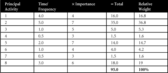
   After doing all the multiplication, sum the total ratings assigned to each principal activity (95 in the preceding example). Then divide the total rating for each principal activity by sum, or all the ratings, to derive the relative weight for the activity (for example, 16 ÷ 95 = 0.168, or 16.8 percent). Knowing each principal activity’s relative weight allows us to allocate proportional shares of the employee’s overall salary to each principal activity, as is done in step 4.

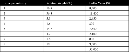
4. Assign dollar values to each principal activity. Take an average (or weighted average) annual rate of pay for all participants in the study (employees in a particular job class) and allocate it across principal activities according to the relative weights obtained in step 3.
   

   To illustrate, suppose that the annual salary of each accounting supervisor is $50,000.

   
5. Rate performance on each principal activity on a 0–200 scale. Note that steps 1–4 apply to the job, regardless of who does that job. The next task is to determine how well each person in that job performs each principal activity. This is the performance appraisal phase. The higher the rating on each principal activity, the greater the economic value of that activity to the organization.
   

   CREPID uses a modified magnitude-estimation scale to obtain information on performance.⁴³ To use this procedure, a value (say, 1.0) is assigned to a referent concept (for example, the average employee, one at the 50th percentile on job performance), and then all comparisons are made relative to this value. In the study of accounting supervisors, operating managers indicated that even the very best employee was generally not more than twice as effective as the average employee. Thus, a continuous 0–2.0 scale was used to rate each employee on each principal activity.

6. Multiply the point rating (expressed as a decimal number) assigned to each principal activity by the activity’s dollar value. To illustrate, suppose that the following point totals are assigned to accounting supervisor C. P. Ayh:
   
   
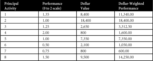
7. Compute the overall economic value of each employee’s job performance by adding the last column of step 6. In our example, the overall economic value of Mr. Ayh’s job performance is $57,902.50, or $7,902.50 more than he is being paid.
8. Over all employees in the study, compute the mean and standard deviation of dollar-valued job performance. When CREPID was tested on 602 first-level managers at a Bell operating company, the mean of dollar-valued job performance was only $2,340 (3.4 percent) more than the average actual salary of all employees in the study. However, the standard deviation (SD_y) was almost $23,791 (all figures in 2010 dollars), which was more than three and a half times larger than the standard deviation of the actual distribution of salaries. Such high variability suggests that supervisors recognized significant differences in performance throughout the rating process.
   

   It is important to point out that CREPID requires only two sets of ratings from a supervisor:

   • A rating of each principal activity in terms of time/frequency and importance (the job analysis phase)

   • A rating of a specific subordinate’s performance on each principal activity (the performance appraisal phase)

   CREPID has the advantage of assigning each employee a specific value that can be analyzed explicitly for appropriateness and that may also provide a more understandable or credible estimate for decision makers. Focusing attention on elements of a job allows leaders to discuss the relative pivotalness of those elements. This idea has proven useful in considering how to apply engineering concepts such as Kano analysis to calculate the value of employee performance.⁴⁴ For example, consider the engineers at a Disney theme park. Unlike typical thrill-ride parks, the designers of Disney rides must be much more attuned to imagery, songs, and stories, because Disney uses the songs, characters, and stories of its rides across its full gamut of products. Consider that the hit film Pirates of the Caribbean began as a ride at Disneyland.

   Hence, for a Disney ride designer (or “imagineer,” as they are called at Disney), the difference between being good and great at songs may be much more pivotal than being good versus great at ride physiology. The ride It’s A Small World has a song that is immediately recognizable all across the world, but its engineering sophistication is not that high. Thus, for Disney, ride engineers might be hired and rewarded more for great songs and stories than for the most advanced thrill-ride capability. CREPID would assign a much higher weight to the music than the physiology design elements of Disney engineers. At a more traditional thrill-ride park, such as Cedar Point in Ohio, the opposite might be true.⁴⁵

   However, as noted earlier, CREPID assumes that average wage equals the economic value of a worker’s performance. This assumption is used in national income accounting to generate the GNP and labor-cost figures for jobs where output is not readily measurable (for example, government services). That is, the same value is assigned to both output and wages. Because this assumption does not hold in pay systems that are based on rank, tenure, or hourly pay rates, CREPID should not be used in these situations.⁴⁶

Logic

In essence, it calculates the difference in system effectiveness between the average performer and someone who is one standard deviation better than average. It multiplies that value by the cost of the system, assuming that the superior performer achieves higher performance using the same cost, or that the superior performer achieves the same performance level at less cost. For example, suppose we estimate that a superior performer (one standard deviation better than average) is 20 percent better than an average performer and that it costs $100,000 to run the system for a month. We multiply the 20 percent by $100,000 to get $20,000 per month as the monetary difference between superior and average performers. The assumption is that the superior performer saves us $20,000 per month to achieve the same results, or that he or she achieves $20,000 more per month using the same cost of capital.

This approach distinguishes the standard deviation of performance in dollars, from the standard deviation of output units of performance (for example, number of hits per firing from an army tank commander). It is based on the following equation.

9-3.

Here, C_u is the cost of the unit in the system. (It includes equipment, support, and personnel rather than salary alone.) Y₁ is the mean performance in output units. Equation 9-3 indicates that the SD of performance in monetary units equals the cost per unit times the ratio of the SD of performance in output units to the average level of performance, Y₁. However, estimates from Equation 9-3 are appropriate only when the performance of the unit in the system is largely a function of the performance of the individual in the job.

Measures

To assess the standard deviation of performance in monetary units, using the system-effectiveness technique, researchers collected data on U.S. Army tank commanders.⁴⁸ They obtained these data from technical reports of previous research and from an approximation of tank costs. Previous research indicated that meaningful values for the ratio SD_y/Y₁ range from 0.2 to 0.5. Tank costs, consisting of purchase costs, maintenance, and personnel, were estimated to fall between $739,674 and $1.23 million per year (in 2010 dollars). For purposes of Equation 9-1, C_u was estimated at $739,674 per year, and the ratio of SD of performance in output units/Y₁ was estimated at 0.2. This yielded the following:

SD of performance in dollars = $739,674 × 0.2 = $147,935

Logic

The first step is to estimate the number (N85) of 85th-percentile employees required to equal the performance of some fixed number (N50) of average performers. Where the value of average performance (V50) is known or can be estimated, SD_y may be estimated by using the ratio N50 / N85 times V50 to obtain V85, and then subtracting V50. That reduces as follows:

9-4.

But by definition, the total value of performance at a certain percentile is the product of the number of performers at that level times the average value of performance at that level, as follows:

9-5.

Combining Equations 9-4 and 9-5 yields this:

9-6.

Measures

The researchers developed a questionnaire to obtain an estimate of the number of tanks with superior tank commanders needed to equal the performance of a standard company of 17 tanks with average commanders.⁴⁹ A fill-in-the-blanks format was used, as shown in the following excerpt.

For the purpose of this questionnaire an “average” tank commander is an NCO or commissioned officer whose performance is better than about half his fellow TCs. A “superior” tank commander is one whose performance is better than 85% of his fellow tank commanders.

The first question deals with relative value. For example, if a “superior” clerk types ten letters a day and an “average” clerk types five letters a day then, all else being equal, five “superior” clerks have the same value in an office as ten “average” clerks. In the same way, we want to know your estimate or opinion of the relative value of “average” vs. “superior” tank commanders in combat. I estimate that, all else being equal, _______________ tanks with “superior” tank commanders would be about equal in combat to 17 tanks with “average” tank commanders.

Questionnaire data was gathered from 100 tank commanders enrolled in advanced training at a U.S. Army post. N50 was set at 17 as a fixed number of tanks with average commanders, because a tank company has 17 tanks. Assuming that organizations pay average employees their approximate worth, the equivalent civilian salary for a tank commander was set at $73,535 (in 2010 dollars).

The median response given for the number of superior TCs judged equivalent to 17 average TCs was 9, and the mode was 10. The response 9 was used as most representative of central tendency. Making use of Equation 9-3, V85 was calculated as follows:

($73,535 × 17) / 9 = $138,899

In terms of Equation 9-4:

SD_y = $73,535 [(17 ÷ 9)-1] = $65,364

This is considerably less than the SD$ value ($136,800) that resulted from the system effectiveness technique. SD_y also was estimated using the global estimation procedure. However, there was minimal agreement either within or between groups for estimates of superior performance, and the distributions of the estimates for both superior performance and for average performance were skewed positively. Such extreme response variability illustrates the difficulty of making these kinds of judgments when the cost of contracting work is unknown, equipment is expensive, or other financially intangible factors exist. Such is frequently the case for public employees, particularly when private-industry counterparts do not exist. Under these circumstances, the system effectiveness technique or the superior equivalents technique may apply.

One possible problem with both of these techniques is that the quality of performance in some situations may not translate easily into a unidimensional, quantitative scale. For example, a police department may decide that the conviction of one murderer is equivalent to the conviction of five burglars. Whether managers do, in fact, develop informal algorithms to compare the performance of different individuals, perhaps on different factors, is an empirical question. Certainly, the performance dimensions that are most meaningful and useful will vary across jobs.

This completes our examination of five different methods for estimating the economic value of job performance. Researchers have proposed variations of these methods,⁵⁰ but at this point, the reader might naturally ask whether any one method is superior to the others. Our final section addresses that question.

As discussed in Chapter 2, “Analytical Foundations of HR Measurement,” if the question is reframed from “How much is this program worth?” to “How likely is it that this investment will reach at least a minimum acceptable level of return?,” the process of making the correct decision is often much more logical, so better decisions are more likely. In terms of SD_y, this means that it is often the case that even a wide range of SD_y values will yield the same conclusion—namely, that what appeared to be very costly HR program investments are actually quite likely to pay off. In fact, the break-even level of SD_y (the level needed to meet the minimal acceptable level of return) is often lower than even the most conservative SD_y estimates produced by the techniques described here.

A review of 34 studies that included more than 100 estimates of SD_y concluded that differences among alternative methods for estimating SD_y are often less than 50 percent.⁵¹ Even though differences among methods for estimating SD_y may be small, those differences can become magnified when multiplied by the number of persons selected, the validity, and the selection ratio. Without any meaningful external criterion against which to compare SD_y estimates, we are left with little basis for choosing one method over another. This is what led the authors of one review to state, “Rather than focusing so much attention on the estimation of SD_y, we suggest that utility researchers should focus on understanding exactly what Y represents.”⁵²

In terms of the perceived usefulness of the utility information, research has found that different SD_y techniques influence managers’ reactions differently (the 40 percent rule was perceived as more credible than CREPID), but these differences accounted for less than 5 percent of the variance in the reactions.⁵³ At a broader level, another study found that managers preferred to receive information about the financial results of HR interventions rather than anecdotal information, regardless of the overall impact of such programs (low, medium, or high).⁵⁴

Utility analyses should reflect the context in which decisions are made.⁵⁵ For example, is the task to choose among alternative selection procedures? Or is it to decide between funding selection program or buying new equipment? All utility analyses involve uncertainty and risk, just like any other organizational measurement. By taking uncertainty into account through sensitivity or break-even analysis (see Chapter 2), any of the SD_y estimation methods may be acceptable because none yields a result so discrepant as to change the decision in question. Instead of fixating on accuracy in estimating SD_y, HR and business leaders should use the logic of performance variability to understand where it matters. If a wide range of values yields the same decision, debating the values is not productive.

The broader issue requires answers to questions such as the following: Where would improvements in talent, or how it is organized, most enhance sustainable strategic success? We began this chapter by focusing on performance-yield curves and the notion of pivotal talent. We emphasized that it is important to distinguish average value from variability in value, and that a key question for managers is not which talent has the greatest average value, but rather, in which talent pools performance variation creates the biggest strategic impact. The estimation of SD_y provides an answer to one important piece of that puzzle.

It is important that HR and business leaders also attend to the larger question. Beyond simply the slope of the performance-value curve (reflected in SD_y), the shape of the curves can be informative. In what jobs or roles is performance at standard good enough? In what jobs or roles is the issue to reduce risk, not necessarily to improve performance levels (such as airline pilots, and nuclear plant operators)? Conversely, in what jobs or roles can downside risk be accepted, for the chance that innovation and creativity create great value (such as Starbucks baristas)? Traditional approaches to job analysis, goal setting and performance management tend to overlook these questions. Yet it is within these processes that HR and business leaders often have the greatest opportunity to understand deeply not only the dollar value of performance differences (SD_y), but the very nature of how work performance contributes to organizational value.⁵⁶

Sometimes it is best to start at a less complex high level. For example, the IBM Institute for Business Value interpreted the idea of “pivotal roles” to recommend that organizations define and distinguish focal jobs defined as “positions that make a clear and positive difference in a company’s ability to succeed in the marketplace.” The Institute authors suggest developing “heat maps” that identify which parts of a business are core (necessary to stay in business but not differentiating in the marketplace), competitive (gets the organization considered by a potential customer), and differentiating (significantly influences the buying decisions of customers). The idea is that performance variation in the “competitive” and “differentiating” parts of the organization is likely to be more valuable than in the “core.”⁵⁷ Figure 9-4 is an example of such a heat map.

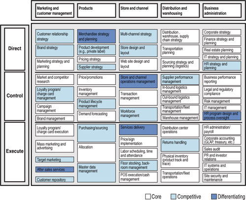
Figure 9-4. Heat map showing what organization processes are most differentiating.

Even such a simple categorization can start a valuable conversation about performance variation and what it means. Then the tools described here can be used to get more specific, attaching consequences and perhaps even monetary values to such performance differences. The next chapter provides an example of embedding the value of performance within a specific decision framework, by applying utility analyses to employee selection. The chapter will also show the role of economic factors, employee flows, and break-even analysis in interpreting such results.

1. Divide into four- to six-person teams and do either A or B, depending on feasibility.
   

   A. Choose a production job at a fast-food restaurant and, after making appropriate modifications of the standard-costing approach described in this chapter, estimate the mean and standard deviation of dollar-valued job performance.

   B. The Tiny Company manufactures components for word processors. Most of the work is done at the 2,000-employee Tiny plant in the Midwest. Your task is to estimate the mean and standard deviation of dollar-valued job performance for Assemblers (about 200 employees). You are free to make any assumptions you like about the Tiny Assemblers, but be prepared to defend your assumptions. List and describe all the factors (along with how you would measure each one) that your team would consider in using standard costing to estimate SD_y.

2. Jim Hill is the manager of subscriber accounts for the Prosper Company. The results of a job analysis indicate that Jim’s job includes four principal activities. A summary of Jim’s superior’s ratings of the activities and Jim’s performance of each of them follows:
   
   

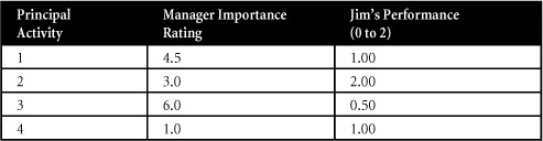
   Assuming that Jim is paid $62,000 per year, use CREPID to estimate the overall economic value of his job performance.

3. Assume that an average SWAT team member is paid $55,000 per year. Complete the following questionnaire. Then use the results to estimate SD_y by means of the superior equivalents technique.
   

   For purposes of this questionnaire, a “superior” SWAT team member is one whose performance is better than about 85 percent of his fellow SWAT team members. Please complete the following item:

   I estimate that, all else being equal, _________ “superior” SWAT team members would be about equal to 20 “average” SWAT team members.

1. Tam, P. W., and K. J. Delaney, “Talent Search: Google’s Growth Helps Ignite Silicon Valley Hiring Frenzy,” The Wall Street Journal (November 23, 2005), A1.

2. Boudreau, John W., Retooling HR: Using Proven Business Tools to Make Better Decisions About Talent (Boston: Harvard Business Press, 2010).

3. Boudreau, 2010; Boudreau, J. W., and P. M. Ramstad, “Strategic Industrial and Organizational Psychology and the Role of Utility Analysis Models,” in Handbook of Psychology, Volume 12, Industrial and Organizational Psychology, ed. W. C. Borman, D. R. Ilgen, and R. J. Klimoski (Hoboken, N.J.: Wiley, 2003).

4. Boudreau, J. W., and P. Ramstad, Beyond HR: The New Science of Human Capital (Boston: Harvard Business School Press, 2007).

5. A more complete treatment of the Disney example, as well as the concept of pivotalness and performance-yield curves, can be found in Boudreau and Ramstad, 2007.

6. Cabrera, E. F., and J. S. Raju, “Utility Analysis: Current Trends and Future Directions,” International Journal of Selection and Assessment 9 (2001): 92–102.

7. Hunter, J. E., F. L. Schmidt, and M. K. Judiesch, “Individual Differences in Output Variability As a Function of Job Complexity,” Journal of Applied Psychology 75 (1990): 28–42.

8. Boudreau and Ramstad, 2007.

9. Ibid.

10. Ibid.

11. Boudreau, 2010.

12. Kano, Noriaki, Nobuhiku Seraku, Fumio Takahashi, and Shinichi Tsuji, “Attractive Quality and Must-Be Quality,” Journal of the Japanese Society for Quality Control 14, no. 2 (April 1984): 39–48. http://ci.nii.ac.jp/Detail/detail.do?LOCALID=ART0003570680&lang=en.

13. Boudreau, 2010.

14. Cronbach, L. J., and G. C. Gleser, Psychological Tests and Personnel Decisions, 2nd ed. (Urbana, Ill.: University of Illinois Press, 1965). See also Raju, N. S., M. J. Burke, and J. Normand, “A New Approach for Utility Analysis,” Journal of Applied Psychology 75 (1990): 3–12; and Boudreau and Ramstad, 2003.

15. Brogden, H. E., and E. K. Taylor, “The Dollar Criterion—Applying the Cost Accounting Concept to Criterion Construction,” Personnel Psychology 3 (1950): 133–154.

16. Brogden, H. E., and E. K. Taylor, “The Dollar Criterion—Applying the Cost Accounting Concept to Criterion Construction,” Personnel Psychology 3 (1950): 133–154.

17. Greer, O. L., and W. F. Cascio, “Is Cost Accounting the Answer? Comparison of Two Behaviorally Based Methods for Estimating the Standard Deviation of Job Performance in Dollars with a Cost Accounting–Based Approach,” Journal of Applied Psychology 72 (1987): 588–595.

18. Horngren, C. T., G. M. Foster, S. M. Datar, and Madhav V. Rajan, Cost Accounting: A Managerial Emphasis, 13th ed. (Upper Saddle River, N.J.: Prentice Hall, 2008). See also Cherrington, J. O., E. D. Hubbard, and D. Luthy, Cost and Managerial Accounting (Dubuque, Ia.: Wm. C. Brown, 1985).

19. Time-period dollar conversions were calculated using the U.S. Consumer Price Index approach and the calculator at the Bureau of Labor Statistics website (http://data.bls.gov/cgi-bin/cpicalc.pl).

20. Schmidt, F. L., and J. E. Hunter, “Individual Differences in Productivity: An Empirical Test of Estimates Derived from Studies of Selection Procedure Utility,” Journal of Applied Psychology 68 (1983): 407–414.

21. Subsequent research indicates that this guideline is quite conservative. See Judiesch, M. K., F. L. Schmidt, and K. K. Mount, “An Improved Method for Estimating Utility,” Journal of Human Resource Costing and Accounting 1, no. 2 (1996): 31–42.

22. Hunter, Schmidt, and Judiesch, 1990.

23. Boudreau, J. W., “Utility Analysis,” in Human Resource Management: Evolving Roles and Responsibilities, ed. L. Dyer (Washington, D.C.: Bureau of National Affairs, 1988).

24. Schmidt, F. L., J. E. Hunter, R. C. McKenzie, and T. W. Muldrow, “Impact of Valid Selection Procedures on Workforce Productivity,” Journal of Applied Psychology 64 (1979): 610–626.

25. In a normal distribution of scores, + 1SD corresponds approximately to the difference between the 50th and 85th percentiles, and –1SD corresponds approximately to the difference between the 50th and 15th percentiles.

26. Schmidt, Hunter, McKenzie, and Muldrow, 1979.

27. Boudreau and Ramstad, 2008.

28. Schmidt, Hunter, McKenzie, and Muldrow, 1979.

29. Judiesch, M. K., F. L. Schmidt, and M. K. Mount, “Estimates of the Dollar Value of Employee Output in Utility Analyses: An Empirical Test of Two Theories,” Journal of Applied Psychology 77 (1992): 234–250.

30. Ibid. See also Judiesch, M. K., F. L. Schmidt, and M. K. Mount, “An Improved Method for Estimating Utility,” Journal of Human Resource Costing and Accounting 1, no. 2 (1996): 31–42.

31. Hunter, Schmidt, and Judiesch, 1990.

32. Judiesch, Schmidt, and Mount, 1996.

33. Judiesch, Schmidt, and Mount, 1992.

34. Cesare, S. J., M. H. Blankenship, and P. W. Giannetto, “A Dual Focus of SD_y Estimations: A Test of the Linearity Assumption and Multivariate Application,” Human Performance 7, no. 4 (1994): 235–255.

35. Burke, M. J., and J. T. Frederick, “Two Modified Procedures for Estimating Standard Deviations in Utility Analyses,” Journal of Applied Psychology 69 (1984): 482–489; Lezotte, D. V., N. S. Raju, M. J. Burke, and J. Normand, “An Empirical Comparison of Two Utility Analysis Models,” Journal of Human Resource Costing and Accounting 1, no. 2 (1996): 110–130; and Rich, J. R., and J. W. Boudreau, “The Effects of Variability and Risk on Selection Utility Analysis: An Empirical Simulation and Comparison,” Personnel Psychology 40 (1987): 55–84.

36. Boudreau and Ramstad, 2007.

37. Desimone, R. L., R. A. Alexander, and S. F. Cronshaw, “Accuracy and Reliability of SD_y Estimates in Utility Analysis,” Journal of Occupational Psychology 59 (1986): 93–102

38. Bobko, P., R. Karren, and J. J. Parkington, “The Estimation of Standard Deviations in Utility Analyses: An Empirical Test,” Journal of Applied Psychology 68 (1983): 170–176; Burke and Frederick, 1984; and Burke, M. J., and J. T. Frederick, “A Comparison of Economic Utility Estimates for Alternative Rational SD_y Estimation Procedures,” Journal of Applied Psychology 71 (1986): 334–339.

39. Greer and Cascio, 1987.

40. Lezotte et al., 1996.

41. Cascio, W. F., and R. A. Ramos, “Development and Application of a New Method for Assessing Job Performance in Behavioral/Economic Terms,” Journal of Applied Psychology 71 (1986): 20–28.

42. Weekley, J. A., B. Frank, E. J. O’Connor, and L. H. Peters, “A Comparison of Three Methods of Estimating the Standard Deviation of Performance in Dollars,” Journal of Applied Psychology 70 (1985): 122–126.

43. Stevens, S. S., “Issues in Psychophysical Measurement,” Psychological Review 78 (1971): 426–450.

44. Boudreau and Ramstad, 2007; Boudreau, 2010.

45. Ibid.

46. Boudreau, J. W., “Utility Analysis for Decisions in Human Resource Management,” in Handbook of Industrial and Organizational Psychology, Volume 2, 2nd ed., ed. M. D. Dunnette and L. M. Hough (Palo Alto, Calif.: Consulting Psychologists Press, 1991).

47. Eaton, N. K., H. Wing, and K. J. Mitchell, “Alternate Methods of Estimating the Dollar Value of Performance,” Personnel Psychology 38 (1985): 27–40.

48. Ibid.

49. Ibid.

50. Raju, Burke, and Normand, 1990; Judiesch, M. K., F. L. Schmidt, and J. E. Hunter, “Has the Problem of Judgment in Utility Analysis Been Solved?” Journal of Applied Psychology 78 (1993): 903–911; and Law, K. S., and B. Myors, “A Modification of Raju, Burke, and Normand’s (1990) New Model for Utility Analysis,” Asia Pacific Journal of Human Resources 37, no. 1 (1999): 39–51.

51. Boudreau, 1991.

52. Arvey, R. D., and K. R. Murphy, “Performance Evaluation in Work Settings,” Annual Review of Psychology 49 (1998): 141–168.

53. Hazer, J. T., and S. Highhouse, “Factors Influencing Managers’ Reactions to Utility Analysis: Effects of SD_y Method, Information Frame, and Focal Intervention,” Journal of Applied Psychology 82 (1997): 104–112.

54. Mattson, B. W., “The Effects of Alternative Reports of Human Resource Development Results on Managerial Support,” Human Resource Development Quarterly 14, no. 2 (2003): 127–151.

55. Cascio, W. F., “The Role of Utility Analysis in the Strategic Management of Organizations,” Journal of Human Resource Costing and Accounting 1, no. 2 (1996): 85–95; Cascio, W. F., “Assessing the Utility of Selection Decisions: Theoretical and Practical Considerations,” in Personnel Selection in Organizations, ed. N. Schmitt and W. C. Borman (San Francisco: Jossey-Bass, 1993): 39–335; and Russell, C. J., A. Colella, and P. Bobko, “Expanding the Context of Utility: The Strategic Impact of Personnel Selection,” Personnel Psychology 46 (1993): 781–801.

56. Boudreau, 2010.

57. Lesser, Eric, Denis Brousseau, and Tim Ringo, Focal Jobs: Viewing Talent through a Different Lens (Somers, N.Y.: IBM Institute for Business Value, 2009).