Chapter 10. The Payoff from Enhanced Selection

Have you ever made a profit from a catering business or dog walking? Do you prefer to work alone or in groups? Have you ever set a world record in anything? The right answer might help you get a job at Google, Inc. Google received more than 100,000 job applications every month in 2007, and to deal with that volume of applications, Google created an algorithm that sifts through answers to an elaborate online survey. The answers are fed into a series of formulas created by Google’s mathematics experts that calculate a score between 0 and 100 to “predict how well a person will fit into its chaotic and competitive culture.” Lazlo Bock, Google’s vice president for people operations, joined Google in spring 2006 and found the selection process rejecting candidates with engineering GPAs of less than 3.7 out of 4.0, and taking two months to consider candidates because each one was submitted to more than half a dozen interviews. After analyzing survey questions as diverse as pet ownership, magazine subscriptions, and introversion, and comparing them with work performance factors as diverse as job rating and organizational citizenship, Google found that “too much schooling can be a detriment” in some jobs. The company created different surveys for candidates in different areas, such as engineering, sales, finance, and human resources.¹

Is it worth it to invest so much time and energy into this system? Are the cost savings from the online approach actually worth it, or does Google give up lots of value by foregoing the half-dozen interviews? Recall from Chapter 9, “The Economic Value of Job Performance,” that Alan Eustace, Google’s vice president of engineering, told The Wall Street Journal that one top-notch engineer is worth 300 times or more than the average and that he would rather lose an entire incoming class of engineering graduates than one exceptional technologist.² Should Google be selecting more carefully for its technologists than engineers? The tools in this chapter are designed to answer questions like these.

Chapter 8, “Staffing Utility: The Concept and Its Measurement,” provided you with the logical and mathematical models for calculating the utility of staffing. Chapter 9 showed how to estimate an important element of staffing utility models: the monetary value of the standard deviation of performance. When you put the models of Chapter 8 together with the estimates of Chapter 9, you end up with powerful analytical frameworks that help predict when investments in enhanced selection will pay off. Lacking the frameworks provided here, organization leaders often see only the costs of such programs. Or, well-meaning psychologists present leaders with statistics such as validity coefficients out of context. Decision makers may ignore the difficult-to-understand value of improved selection and instead focus only on the costs, which often causes them to forego valuable opportunities.

By the same token, staffing professionals often become so focused on improving the elegance of staffing systems that they lose sight of the need to balance costs and benefits. Improved validity in employee selection is not always worth the cost, and it is certainly not equally valuable in every situation. The logic of Chapter 8 and the estimation methods of Chapter 9 combine to provide clues about where staffing investments have the greatest payoff.

Employee selection is quite similar to other business processes. In essence, investing in employee selection is an example of gathering information to improve our ability to predict the performance of a risky asset. In this case, the “asset” is a new hire, but the logic of the decision is the same logic that supports decisions to invest in research on financial investments, mineral exploration, consumer preferences, and any other uncertain resource.

In Chapter 8 (Figure 8-1), we introduced the idea of a supply chain approach to staffing, showing that the pipeline of talent is very similar to the pipeline of any other resource. At each stage, the candidate pool can be thought of in terms of the quantity of candidates, the average and dispersion of the quality of the candidates, and the cost of processing and employing the candidates. Quantity, quality, and cost considerations determine the monetary value of staffing programs, and the utility models of Chapter 8 showed how to calculate and combine these factors.

In this chapter, we tie these ideas together to show how to actually calculate the value of improved employee selection and other aspects of the talent supply chain.³ We show how valid selection procedures (for external and internal candidates) can pay off handsomely for organizations. Moreover, we show how the basic utility formulas can incorporate important financial considerations, to make utility estimates more comparable with estimates of investment returns for other resources such as technology, advertising, and so on.

To date, utility analysis has not been used widely. Yet it has the potential to provide an answer to the increasing calls for greater rigor and economic justification for HR investments (see Chapter 1, “Making HR Measurement Strategic”). This chapter shows how to make utility analysis estimates compatible with other financial estimates, which we believe will make it easier for HR leaders to “retool” utility analysis within the logic of proven business tools.⁴ Thus, business leaders will develop shared mental models and make better decisions about staffing and other HR programs.

We begin with an example of tangible results from improved staffing, estimated with the Brogden-Cronbach-Gleser model described in Chapter 8.⁵ Then we consider the effects of five considerations that help make staffing payoffs more realistic and better connected to traditional financial logic:

• Economic factors (variable costs, taxes, and discounting)

• Employee flows

• Probationary periods

• The use of multiple selection devices

• Departures from top-down hiring

Then we address the issue of risk and uncertainty in utility analysis and offer several tools to aid in decision making. We conclude the chapter by focusing on processes used to communicate the results of utility analyses to decision makers.

Figure 10-1. The logic of utility analysis and factors that can affect payoffs.

We discussed several of these factors in Chapters 8 and 9. In Chapter 8, Equation 8-17 showed how the Brogden-Cronbach-Gleser model combines several of these factors, namely the selection ratio (SR), the validity of the selection procedure (r), the variability or standard deviation of job performance expressed in monetary terms (SD_y), the average score of those hired on the predictor, and the average cost per selectee of applying the selection process to all applicants [(N_a × C)/N_s], to determine an unadjusted estimate of the utility of a selection process. The remaining factors shown in Figure 10-1 may increase or decrease the unadjusted utility estimate. We discuss each of them after we illustrate the computation of the unadjusted estimate in the following section.

In terms of quantity, the average number of GS-5 through GS-9 programmers selected was 618 per year. Estimating on the basis of U.S. census data in 1979, 10,210 computer programmers could be hired each year in the U.S. economy using the PAT. The average tenure for government programmers was found to be 9.69 years; in the absence of other information, this tenure figure was assumed for the private sector as well. The average gain in utility per selectee per year was multiplied by 9.69 to yield a total employment period gain in utility per selectee.

It was not possible to determine the prevailing selection ratio (SR) for computer programmers either in the general economy or in the federal government, so the utility analysis formula was used to do sensitivity analysis using an SR of 0.05 and then substituting SRs in intervals of 0.10 from 0.10 to 0.80.

In terms of validity, it’s possible for the PAT to replace a prior procedure with zero validity in some cases, but in other situations, the PAT replaced a procedure with lower but nonzero validity. Thus, utilities were calculated assuming previous-procedure true validities of 0.20, 0.30, 0.40, and 0.50, as well as zero.

SDy was calculated as the average of the two estimates obtained from experts, using the global estimation procedure described in Chapter 9. The estimate was $38,613 per person per year (in 2010 dollars).

When the previous procedure was assumed to have zero validity, its associated testing cost also was assumed to be zero. When the previous procedure was assumed to have a nonzero validity, its associated cost was assumed to be the same as that of the PAT (that is, $36 per applicant). Cost of testing was charged only to the first year, as if the procedure was used only once, to select the first group of programmers.

The Brogden-Cronbach-Gleser general utility equation was modified to obtain the equation actually used in computing the utilities.

10-1.

Here, ΔU is the gain in productivity in dollars from using the new selection procedure for one year; t is the tenure in years of the average selectee (here 9.69); N_s is the number selected in a given year (this figure was 618 for the federal government and 10,210 for the U.S. economy); r₁ is the validity of the new procedure, here the PAT (r₁ = 0. 76); r₂ is the validity of the previous procedure (r₂ ranges from 0 to 0.50); c_l is the cost per applicant of the new procedure, here $36; and c₂ is the cost per applicant of the previous procedure, here zero or $36. The terms SD_y, λ, and φ are as defined previously in Chapter 8. This equation gives the productivity gain that results from one year’s use of the new (more valid) selection procedure, but not all these gains are realized the first year; they are spread out over the 9.69-year tenure of the new employees.

To illustrate how those figures were derived, assume that the SR = 0.20 and the previous procedure has a validity of 0.30. All other terms are as defined previously.

ΔU = 9.69(618)(0.76 – 0.30)($38,613)(0.2789 ÷ 0.20) – 618($36 – $36)/0.20

ΔU = 9.69(618)(0.46)($38,613)(1.3945) – 0

ΔU = $148,327,660

The gain per selectee can be obtained by dividing the value of total utility by 618, the assumed yearly number of selectees. When this is done for our example ($148,327,660 / 618), the gain per selectee is $240,012. That figure is still quite high, but remember that not all of those gains are realized during the first year. They are spread out over the entire tenure of the new employees. Gains per year per selectee can be obtained by dividing the total utility first by 618 and then by 9.69, the average tenure of computer programmers. In our example, this produces a per-year gain of $24,769 per selectee—or, to carry it even further, a $12 gain per hour per year per selectee (assuming 2,080 hours per work year). Other research has often produced equally stunning estimates of the monetary value of improved selection.⁸

Figure 10-1 showed that the cost of a selection program depends not only on the number of individuals selected and the cost of selection, but also on several additional economic factors. These include variable costs, taxes, and discounting. Why are these important? By taking them into account, decision makers can evaluate the soundness of HR investments more comparably with other investments. Other financial investments routinely account for these factors, so failing to consider them in estimating the value of staffing produces utility estimates that are overstated compared to other investments. Decision makers will want to compare HR investments on compatible terms with other investments, so these adjustments help make HR utility estimates more comparable.

10-2.

Here, ΔU is the change in overall worth or utility after variable costs, taxes, and discounting; N is the number of employees selected; t is the time period in which an increase in productivity occurs; T is the total number of periods (for example, years) that benefits continue to accrue to an organization; i is the discount rate; SD_sv is the standard deviation of the sales value of productivity among the applicant or employee population (this is similar to SD_y in previous utility models but is called sales value to reflect the idea of translating productivity into the sales revenue it would generate, and to distinguish it from profits); V is the proportion of sales value represented by variable costs; TAX is the organization’s applicable tax rate; r_x,sv is the validity coefficient between predictor (x) and sales value (similar to r_x,y in previous utility models); and C_T is the total selection cost for all applicants (equal to the number selected divided by the selection ratio).

Those economic considerations suggest large potential reductions in unadjusted utility estimates. For example, researchers computed an SD_sv value of $38,613 (in 2010 dollars) in their utility analysis of the PAT.¹¹ Although this may have been appropriate for federal government jobs because the federal government is not taxed, it would not be appropriate for private-sector organizations that face variable costs and taxes.

Assuming that the net effect of variable costs is to reduce gains by 5 percent, V = –0.05. Assuming a marginal tax rate (the tax rate applicable to changes in reported profits generated by a decision) of 45 percent, the after-cost, after-tax, one-year SD_y value is as follows:

(SD_sv) × (1 + V) × (1 – TAX)

($38,613) × (1 – 0.05) × (1 – 0.45) = $20,175

This is 52 percent of the original value.

Now, assuming a financial discount rate of 10 percent, if the average tenure of computer programmers in the federal government was just two years, the appropriate discount factor (DF) adjustment would be as shown in Equation 10-3.

10-3.

Over 10 years, DF = 6.14, but the average tenure of computer programmers in the federal government (at the time of the study) was computed to be 9.69 years. Hence, the appropriate adjustment needed to discount the computed utility values 6.03. So, to reflect discounting, the per-year utility should be multiplied by 6.03, instead of 9.69.

When all three of those factors—variable costs, taxes, and discounting—are considered, the per-selectee utility values over 9.69 years that were reported in the study of computer programmers range from $10,210 (which is [$19.5 million / 618 = $31,553 per selectee × (6.03/9.69) × 0.52]) to $174,886 ($334 million / 618 = $540,453 per selectee × (6.03/9.69) × 0.52).

These values still are substantial, but they are 67 percent lower than the unadjusted values. Such significant effects argue strongly that HR leaders should be careful to make their monetary payoff estimates as compatible as possible with standard investment calculations. Note that the adjustments above multiplied the total to adjust for the discount factor (6.03/9.69) and the combination of variable costs and taxes (52 percent of the unadjusted value). This is because the cost difference was zero. If it was non-zero, the added value elements would be adjusted as shown here, but the cost should be adjusted by the tax rate.

Employee flows into, through, and out of an organization influence the value of a staffing program or any other HR intervention.¹² We showed earlier that failure to consider the effects of variable costs, taxes, and discounting tends to overstate utility estimates. Conversely, failure to consider the effect of employee flows may understate utility estimates. The utility analysis formulas originally introduced reflected a selection program used to hire a single group and often reflected only the first-year effect of those better-selected employees. They expressed the utility of adding one new, better-selected cohort to the existing workforce. Yet in any investment, the cumulative benefit over time is relevant. One would not evaluate an investment in improved quality control for raw materials merely on the first order received. In the same way, selection utility should reflect the cumulative effects on all employees selected over time.

In practice, valid selection programs are reapplied year after year, as employees flow into and out of the workforce. A program’s effects on cohorts hired in later years will occur in addition to its lasting effects on previously hired cohorts. These are additive cohort effects.¹⁴ By altering the terms N and T in Equation 10-2, we can account for the effect of employee flows.

Employee flows generally affect utility through the period-to-period changes in the number of treated employees in the workforce. Note that we use the term “treated employees” to mean employees that are affected by an improved HR program, such as the group hired with an improved test. Such employees are added to a workforce containing existing or untreated employees. The number of treated employees in the workforce k periods in the future (N_k) may be expressed as shown in Equation 10-4.

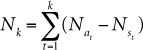
10-4.

Here, is the number of treated employees added to the workforce in period t, and is the number of treated employees subtracted from the work force in period t. For example, consider the makeup of the workforce in the fourth year, after a new selection procedure was applied for four years (k = 4); that 100 persons were hired in each of the four years; and that 10 of them left in Year 2, 15 in Year 3, and 20 in Year 4. The following results are observed from the inception of the program (t = 1) to year 4 (t = 4):

N₄ = (100 – 0) + (100 – 10) + (100 – 15) + (100 – 20)

N₄ = 355

Thus, the term N_k reflects both the number of employees treated in previous periods and their expected separation pattern. The formula for the utility (ΔU_k) occurring in the kth future period that includes the economic considerations of Equation 10-2 may be written as shown in Equation 10-5.

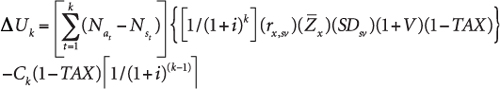
10-5.

This formula modifies the quantity element by keeping track of how many treated employees are in the workforce in each year. Then, after multiplying that number by the increased productive value of the treated employees, the relevant discount rate, cost, tax, and other factors are applied for that particular year.

For simplicity, the utility parameters r_{x, sv}, V, SD_sv, and TAX are assumed to be constant over time. This assumption is not necessary, and sometimes the factors may vary. Note also that the cost of treating (for example, selecting) the N_ak employees added in period k (C_k) is now allowed to vary over time. However, C_k is not simply a constant multiplied by N_ak. Some programs (for example, assessment centers) have high initial startup costs of development, but these costs do not vary with the number treated in future periods. Also, the discount factor for costs [1/(1 + i)^{(k – 1)}] reflects the exponent k – 1, assuming that such costs are incurred one period prior to receiving benefits. Where costs are incurred in the same period as benefits are received, k is the proper exponent.¹⁵

ΔU₄ = (355 × .683 × .40 × .80 × $25,000 × .95 × .55) – ($7,200 × .751 × .55)

× 0.55)] – ($7,200 × .751 × 0.55)

ΔU₄ = $1,013,504 – $2,974 = $1,010,530

$1,013,504 – $2,974 = $1,010,530

This figure equals the total one-year value of the improved performance of all the better selected employees who are still with the organization in the fourth year.

To express the utility of a program’s effects over F periods, the one-period utility estimates (ΔU_k) are summed. Thus, the complete utility model reflecting employee flows through the workforce for a program affecting productivity in F future periods may be written as shown in Equation 10-6.

10-6.

The duration parameter F in Equation 10-6 is not employee tenure, but rather how long a program affects the workforce. Now, let’s apply employee flows to the programmer example, where average tenure was 9.69 years, which we’ll round up to 10 years. Assume that the PAT in the computer programmer study is applied for 15 years, and, for simplicity, assume that each hired group of programmers stays for 10 years. If 618 programmers are added each year, for the first 10 future periods N_k will increase by 618 in each period. For example, in Year 10, 6,180 programmers selected using the PAT have been added to the workforce, and none have left:

10-7.

Beginning in future period 11, however, one PAT-selected cohort leaves in each period ( = 618). However, in Years 11 through 15, by continuing to apply the PAT to select 618 new replacements (that is, = 618), the number of treated programmers in the workforce is maintained. Thus, in Years 11–15, and offset each other and N_k remains unchanged at 6,180. Assuming that the government stops using the test in Year 15, starting in future period 16, the cost and number added (C_k and ) become zero, assuming that the organization returns to random selection. However, the treated portion of the workforce does not disappear immediately. Earlier-selected cohorts continue to separate (that is, = 618), and N_k falls by 618 each period until the last-treated cohort (selected in future period 15) separates in future period 25. Figure 10-2 shows N_k for each of the 25 periods. (In Figure 10-2, F = 25 periods.)

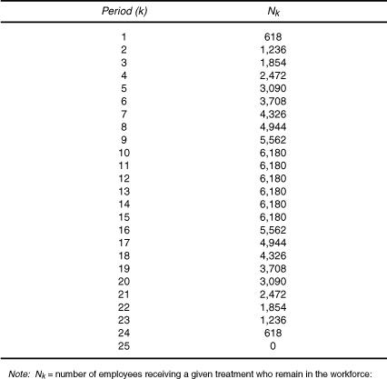
Table 10-2. Example of employee flows over a 25-year period.

Source: Adapted from Boudreau, J. W. (1983). Effects of employee flows on utility analysis of human resource productivity improvement programs. Journal of Applied Psychology 68, 400. Copyright © 1983 by the American Psychological Association. Reprinted with permission.

Now we can add the economic factors to the utility model that reflects employee flows. Assuming, as we did in our earlier example, that V = –0.05, TAX = 0.45, and the discount rate is 10 percent, the total expected utility of the 15-year application of PAT (the sum of the 25 one-period utility estimates, ΔU_k in Equation 10-5) was estimated to be $286.2 million (in 2010 dollars).¹⁶ This is considerably higher than the estimate in the original study of $148.3 million (in 2010 dollars), even after reflecting variable costs, taxes, and discounting.

The most important lesson to learn from the principle of employee flows is that one-cohort utility models often understate actual utility because they reflect only the first part of a larger series of outcomes.

These numbers imply very high payoffs to improved employee selection, when we consider the impact on many employee cohorts over time. It is the same idea as the high cumulative impact of quality control in supply chains, when applied to many years of receiving raw materials orders. The reason the numbers are so high in this case is that the cost of the selection improvement is modest (a test costing less than $50 per applicant), and the difference in value between a good and a very good computer programmer is high ($38,613 per year).

Clearly, this can vary across situations. In the case of Google, at the beginning of this chapter, the cost of developing the algorithm, gathering the online data, analyzing the data, and so on would likely be much higher than $50 per applicant. That said, if the estimate of the value of performance variation among engineers is anywhere near Alan Eustace’s estimate of 300 times, Google can justify even multimillion-dollar selection systems. The point is not so much the precision of the calculation, but the logic and analysis that motivate more productive conversations.

The utility effect of a probationary period is reflected by modifying the utility equation to reflect the difference in performance between the pool of employees hired initially and those who survive the probationary period.¹⁸ Whether a new hire is considered successful depends on his or her performance rating at the end of the probation period.

Because lower performers are dismissed, the average performance of a given selected cohort increases after the probationary period. The actual amount of the improvement depends on two things: the validity of the selection process used to weed out low performers, and the performance cutoff that determines success during probation. The costs of paying and training employees who are later dismissed, together with any separation costs, must also be taken into account among the overall costs of a probationary-hiring program.

Interestingly, a probationary period reduces the harmful effect of selection errors, because they are corrected very quickly. Poor-performing employees are weeded out consistently and early instead of being retained longer in “permanent” positions that require a longer process of formal dismissal. So the value of selection procedures used with a probationary period is less than would be the case if the same selection process were used without the probationary period. Improved selection has value when it reduces hiring errors, but when a probationary period catches those errors, the value of avoiding them is less. Overall, the combined value of improved selection and a probationary period can be higher or lower than using either one alone. It depends on their relative validity, the severity of selection errors, and the variability in the applicant population. All of this is elegantly reflected in the utility model, which can be used to examine these factors in combination to identify the optimum combination.

Another way to look at probationary periods is as a special case of the employee movement model that we described in Chapter 4, “The High Cost of Employee Separations,” in Figure 4-1. In essence, the probationary period is a “controlled turnover” process, in which the validity of the dismissal decision determines the value of turnover to the organization. Finally, when seen this way, it is clear that the combination of selection and probation is much like the supply chain model of Chapter 8, with probation being similar to quality control after raw materials have been accepted and placed into the production process.

A combination of screening raw materials when they arrive and then monitoring their quality as they enter the production process may add great value if the cost of errors is quite high and if a lot of valuable information can be gathered after the materials are in the production process. That’s the same logic Whole Foods is using. By selecting applicants carefully and then having the team observe them as they enter the workplace, Whole Foods is behaving as if the cost of an error is very high and assumes that the team members can see things that the selection process might miss.

Rejecting job offers produces the same effect as reducing hiring standards. It increases SRs and lowers the gains from more valid selection. For example, if an organization needs to select 20 percent of its applicants to fill its positions, but half of its offers get rejected, that is the same as having a 40 percent selection ratio.

In general, offer rejections reduce the value of better selection more when:

• There is a higher correlation between the quality of the applicants and their probability of rejecting the offer.

• There is a larger proportion of rejected job offers.²⁰

How large are the potential losses? One study found, that under realistic circumstances, unadjusted utility formulas could overestimate gains by 30 to 80 percent. To some extent, these utility losses caused by job offer rejection can be offset by additional recruiting efforts that increase the size of the applicant pool and, therefore, restore smaller SRs. Yet if the probability of accepting a job offer is negatively correlated with applicant quality (the better applicants are more likely to reject an offer), increasing the number of applicants may not be as effective as increasing the attractiveness of the organization to the better ones.

Again, the supply chain analogy applies. This is the same tradeoff that must be considered when bidding on scarce production inputs (such as oil field rights and rare components). The organization can increase the number of sellers, make itself more attractive to the sellers (perhaps through pricing or other perks), or a combination of both. As with a supply-chain, the right answer is found by better understanding the variables that determine the value of improved selection and recruitment.

Similar to the effect of rejected offers is the situation in which an organization decides to deviate from the practice of making job offers to the top-scoring candidates. To test this, researchers examined the impact on the productivity of forest rangers of three approaches:

1. Using top-down selection
2. Selecting those who meet a minimum required test score equal to the average
3. Selecting those who meet a minimum required score set at one SD below the average²²

Top-down selection produced a productivity increase of about 13 percent (which translated into millions of dollars) compared to random selection. Under option 2, the value of output gains was only 45 percent as large as the dollar value for top-down selection. Under option 3, the value of output gains was only 16 percent of the top-down figure. Employers who deviate from top-down selection when performance variation is significant do so at substantial economic cost.

The study found that although the unadjusted utility values we’ve seen are quite substantial, the effects of economic factors, departures from top-down hiring, and probationary periods can reduce them substantially. Accounting for economic variables had the largest effect, followed, in rank order, by multiple selection devices, departures from top-down hiring, probationary period, and separations of high performers. The total set of adjustments reduced the utility values by a median level of 91 percent, with a minimum reduction of 71 percent. Thus, considering reasonable values of these adjustments, the remaining utility values might be between 9 percent and 29 percent as large as the unadjusted values. The simulation actually produced negative utility estimates (the costs of improved selection exceeded the benefits) in 16 percent of the cases.

These results suggest that although valid selection procedures may often lead to positive payoffs for the organization, actual payoffs depend significantly on organizational and situational factors that affect the quantity, quality, and cost of the selection effort. The message is that organizations should give careful consideration and analysis to such investments. There is significant potential payoff but also significant potential risk in a poor decision. The tools and formulas in this chapter, together with those in Chapters 8 and 9, provide a framework for improving those decisions.

Meta-analyses of multiple studies often show that the validity of such characteristics as intelligence or conscientiousness for predicting job performance is consistently positive. It is tempting to conclude that hiring based on these factors must invariably contribute to improvements in performance that are worth the investment. However, validity is only one consideration in determining the overall value of a selection system to an organization.

The hallmark of a decision science is its ability to apply consistent frameworks to diverse situations, obtaining different results depending on vital factors. The results of this chapter show that the payoff from improved selection is potentially, but not necessarily, very large. Wise organizations will use the frameworks to examine their particular situations and make sound decisions based on their unique opportunities and constraints.

• It shifts emphasis away from estimating a precise utility value toward making a good decision even with imperfect information.

• It pinpoints areas where controversy is important to decision making (that is, where there is doubt about whether the break-even value is exceeded), versus where controversy has little impact (because there is little risk of observing utility values below break-even).

One comprehensive review of the utility-analysis literature reported break-even values for 42 studies that estimated the parameter SD_y.²⁵ Without exception, the break-even values fell at or below 60 percent of the estimated value of SD_y. In many cases, the break-even value was less than 1 percent of the estimated value of SD_y. This suggests that, in most studies, the precise value of SD_y was not a determining factor in whether better selection paid off. The break-even value is often very low for the choice of whether to implement a particular HR program. However, this simply shows that the HR program is better than nothing. In more realistic settings, when the HR program is compared to other organizational investments, differences in SD_y estimates could actually affect the ultimate decision.²⁶ Also, decision makers may consider uncertainty about other factors (such as validity or selection ratios) in addition to SD_y in making capital-budgeting decisions.²⁷ Nonetheless, break-even analysis can be used in all these situations, and it often helps to clarify what really matters, leading not only to better decisions, but to better logical analysis.

In summary, break-even analysis of the SD_y parameter (or any other single parameter in the utility model) seems to provide two additional advantages:

• It allows practicing managers to appreciate how little variability in job performance is necessary before valid selection procedures begin to pay positive dividends.

• Even if decision makers cannot agree on an exact point estimate of SD_y, they can probably agree that it is higher than the break-even value.

To implement a Monte Carlo analysis, you draw a value for each of the variables from its assumed distribution, input that value into the utility equation, and then calculate the utility value. Doing this repeatedly for many values of the parameters in combination produces an array of utility outcomes. Computer technology permits researchers to run tens of thousands such experimental values. In examining the pattern of resulting utility values, it is possible to estimate the average, range, and likelihood that various utility values will occur.

By modeling and analyzing uncertainty within the Monte Carlo analysis, we can better predict the likely outcomes and the risks of observing very low or very high utility values. To illustrate, the study described earlier was a Monte Carlo analysis that varied all the elements of the utility model with employee flows and economic factors, by analyzing 10,000 scenarios that combined different elements.²⁹

10-8.

Although there are problems with the method used to compute the standard error of the utility estimate, especially the assumption that all components in the equation are independent and normally distributed, research suggests that it provides a serviceable approximation.³¹ To illustrate this method, researchers applied it to the estimated utility of the PAT in predicting the performance of computer programmers in the federal government.³² They found that the values of SE_u were very large, about half the size of the utility estimate itself. This means that the experts who estimated SD_y had less agreement than might have been predicted.

As one observer commented, “Ironically, the impressively large size of utility estimates per se have (sic) been almost overemphasized ... while the standard error of utility has been largely ignored. If we are to be impressed by the size of utility, we must similarly be impressed by the size of the uncertainty in these estimates.”³³ To date, we have tended to view utility values as point estimates rather than as predictions under uncertainty. Given the uncertainty of many of the parameters of the utility model, confidence intervals are probably more appropriate and should be reported routinely.

Research suggests that how utility results are presented makes a big difference. Presented in the wrong way, utility analysis results appear to actually reduce the support of managers for a valid selection procedure, even though the net benefits of the procedure are very large.³⁴ In one experiment, managers were presented with an unadjusted estimated payoff from a selection program of more than $105 million (in 2010 dollars), representing a return on investment of 14,000 percent. Results this large strain credulity, and thus it is no surprise that the managers did not accept them. Moreover, a fundamental principle of financial economics is that high returns carry high risks. Thus, presenting business leaders with such extraordinary estimated returns understandably would cause them to assume that the investment is highly speculative.³⁵ Yet some controversy arises here, because two subsequent studies failed to replicate these findings, and their conclusions and implications have been challenged.³⁶

As we noted earlier, in the section on Monte Carlo analysis, another approach is to provide leaders with a range of possible values. Recall the study described earlier that used a computer-based simulation to generate 10,000 scenarios based on prior research and adjusted for different levels of economic factors and other considerations. The estimates showed an average payoff of $2,964,222 (in 2010 dollars), more than a 96 percent reduction from the unadjusted values. The median return was $2,313,275. The smallest outcome was an estimated loss of $3,428,601, and the largest predicted gain (after adjustment) was $22,831,890. Even this gain was still more than 71 percent smaller than the initial (unadjusted) estimate presented to the non-HR managers.³⁷

Now, with ranges like this, it’s little wonder that many HR leaders, I/O psychologists, and business leaders concluded that estimating the monetary value of enhanced employee selection is mostly guesswork. An investment with a range of values from negative $3 million to positive $23 million may seem like just rolling the dice. However, are business leaders prepared to forego an investment that may produce such a high payoff in fear of the downside?

These are precisely the sorts of decisions that leaders make about other resources. When such uncertainty exists in the face of potentially high payoffs, wise organizations often invest in studies that can make estimates more precise. Using Monte Carlo techniques can show leaders which variables in the utility framework contribute most to the variation in anticipated payoffs. Perhaps organizations could study those variables more deeply and reduce the uncertainty, just as they might do with an uncertain supply chain, customer response to a new product, or R&D pipeline.³⁸

We actually know very little about how decision contexts or organizational characteristics affect the reactions of managers to the results of utility analyses. If we study the thought processes of leaders who make decisions about investments in improved selection or other HR programs, we can learn more about where their beliefs and impressions may be incorrect.³⁹

Beyond those concerns is a genuine need for utility analysts to shift their focus. The fundamental question is not, “How do we construct the best HR measure?” Instead, it is, “How do we induce changes through HR measurement systems?” HR measurement is not an end in and of itself, but rather a decision-support system that can have powerful effects if users pay careful attention to the sender, the receivers, the strategy they use to transmit their message, and the organization of their message.⁴⁰

Evidence indicates that managers are quite receptive to utility analysis when analysts present conservative estimates, illustrate the choices and their advantages and disadvantages, do not overload the presentation with technical details, and emphasize the same concerns managers of operating departments pay attention to (reducing the overall cycle time of the staffing process, reducing costs while maintaining the validity of the overall staffing process).⁴¹ Clearly, the “framing” of the message is critical and has a direct effect on its ultimate acceptability.⁴²

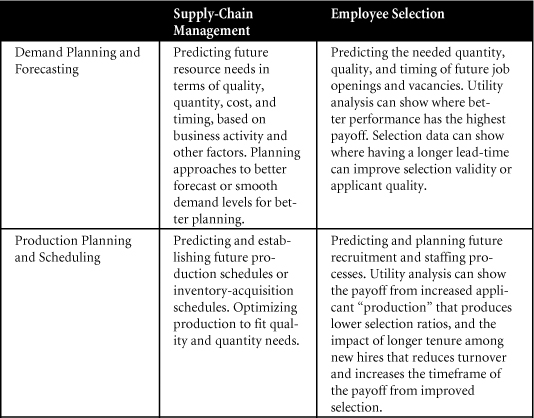
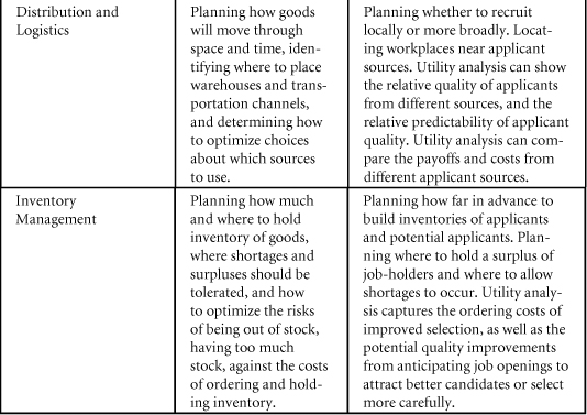
Table 10-1. How Supply-Chain Management and Employee Selection Share Business Logic

These questions are illustrative, and many more parallel ideas exist between traditional supply chains and utility analysis for employee staffing. The point of these illustrations is to encourage HR and business leaders to explore how existing and proven business frameworks can be applied to talent and human capital decisions. The utility analysis framework can seem like a foreign language to most business leaders, but it is largely the same language they already apply to other decisions. It’s just a matter of translation.

1. You are given the following information regarding the CAP test for clerical employees (clerk-2s) at the Berol Corporation:
   

   Average tenure as a clerk-2: 7.26 years

   Number selected per year: 120

   Validity of the CAP test: 0.61

   Validity of previously used test: 0.18

   Cost per applicant of CAP: $35

   Cost per applicant of old test: $18

   SR: 0.50

   Ordinate at SR: 0.399

   SD, in first year: $34,000

   Use Equation 10-1 to determine (a) the total utility of the CAP test, (b) the utility per selectee, and (c) the per-year gain in utility per selectee.

2. Referring to Exercise 1, suppose that after consulting with the chief financial officer at Berol, you are given the following additional information: variable costs are –0.08, taxes are 40 percent, and the discount rate is 8 percent. Use Equation 10-2 in this chapter to recompute the total utility of the CAP test, the utility per selectee, and the utility per selectee in the first year.
3. The Top Dollar Co. is trying to decide whether to use an assessment center to select middle managers for its consumer products operations. The following information has been determined: variable costs are –0.10, corporate taxes are 44 percent, the discount rate is 9 percent, the ordinary selection procedure costs $700 per candidate, the assessment center costs $2,800 per candidate, the standard deviation of job performance is $55,000, the validity of the ordinary procedure is 0.30, the validity of the assessment center is 0.40, the selection ratio is 0.20, the ordinate at that selection ratio is 0.2789, and the average tenure as a middle manager is 3 years. The program is designed to last 6 years, with 20 managers added each year. Beginning in Year 4, however, one cohort separates each year until all hires from the program leave.
   

   Use Equation 10-6 in this chapter to determine whether Top Dollar Co. should adopt the assessment center to select middle managers. What payoffs can be expected in total, per selectee, and per selectee in the first year?

2. Tam, P. W., and K. J. Delaney, “Talent Search: Google’s Growth Helps Ignite Silicon Valley Hiring Frenzy,” The Wall Street Journal (November 23, 2005), A1.

3. Cascio, Wayne F., and John W. Boudreau, “Supply-Chain Analysis Applied to Staffing Decisions,” in Handbook of Industrial and Organizational Psychology, ed. Sheldon Zedeck (Washington, D.C.: American Psychological Association Books, 2010).

4. Boudreau, John W., Retooling HR (Boston: Harvard Business Publishing, 2010).

5. Schmidt, F. L., J. E. Hunter, R. C. Mckenzie, and T. W. Muldrow, “Impact of Valid Selection Procedures on Work-Force Productivity,” Journal of Applied Psychology 64 (1979): 609–626.

6. Ibid.

7. Inflation adjustments were made using the CPI inflation calculator from the U.S. Bureau of Labor Statistics, at http://data.bls.gov/cgi-bin/cpicalc.pl.

8. Boudreau, J. W., “Utility Analysis,” in Human Resource Management: Evolving Roles and Responsibilities, ed. L. Dyer (Washington, D. C.: Bureau of National Affairs, 1988).

9. Boudreau, J. W., “Economic Considerations in Estimating the Utility of Human Resource Productivity Improvement Programs,” Personnel Psychology 36 (1983a): 551–576.

10. Boudreau, J. W., “Effects of Employee Flows on Utility Analysis of Human Resource Productivity Improvement Programs,” Journal of Applied Psychology 68 (1983b): 396–406.

11. Schmidt et al., 1979.

12. Boudreau, J. W., and C. J. Berger, “Decision-Theoretic Utility Analysis Applied to Employee Separations and Acquisitions,” Journal of Applied Psychology Monograph 70, no. 3 (1985): 581–612.

13. Schmidt et al., 1979.

14. Boudreau, 1983b.

15. Ibid.

16. Ibid.

17. www.wholefoodsmarket.com/careers/hiringprocess.php.

18. De Corte, W., “Utility Analysis for the One-Cohort Selection-Retention Decision with a Probationary Period,” Journal of Applied Psychology 79 (1994): 402–411.

19. Becker, B. E., “The Influence of Labor Markets on Human Resources Utility Estimates,” Personnel Psychology 42 (1989): 531–546.

20. Murphy, K. R., “When Your Top Choice Turns You Down: Effects of Rejected Offers on the Utility of Selection Tests,” Psychological Bulletin 99 (1986): 133–138.

21. Cascio, W. F., and H. Aguinis, Applied Psychology in Human Resource Management, 6th ed. (Upper Saddle River, N.J.: Prentice-Hall, 2005).

22. Schmidt, F. L., M. J. Mack, and J. E. Hunter, “Selection Utility in the Occupation of U.S. Park Ranger for Three Modes of Test Use,” Journal of Applied Psychology 69 (1984): 490–497.

23. Sturman, M. C., “Implications of Utility Analysis Adjustments for Estimates of Human Resource Intervention Value,” Journal of Management 26 (2000): 281–299.

24. Cascio, W. F., “Assessing the Utility of Selection Decisions: Theoretical and Practical Considerations,” in Personnel Selection in Organizations, ed. N. Schmitt and W. C. Borman (San Francisco: Jossey-Bass, 1993).

25. Boudreau, J. W., “Utility Analysis for Decisions in Human Resource Management,” In Handbook of Industrial and Organizational Psychology (Vol. 2, 2nd ed.), ed. M. D. Dunnette and L. M. Hough (Palo Alto, CA: Consulting Psychologists Press, 1991).

26. Weekley, J. A., E. J. O’Connor, B. Frank, and L. W. Peters, “A Comparison of Three Methods of Estimating the Standard Deviation of Performance in Dollars,” Journal of Applied Psychology 70 (1985): 122–126.

27. Hoffman, C. C., and G. C. Thornton III, “Examining Selection Utility Where Competing Predictors Differ in Adverse Impact,” Personnel Psychology 50 (1997): 455–470.

28. Sturman, 2000. See also Rich, J. R., and J. W. Boudreau, “The Effects of Variability and Risk on Selection Utility Analysis: An Empirical Simulation and Comparison,” Personnel Psychology 40 (1987): 55–84.

29. Sturman, 2000.

30. Alexander, R. A., and M. R. Barrick, “Estimating the Standard Error of Projected Dollar Gains in Utility Analysis,” Journal of Applied Psychology 72 (1987): 475–479.

31. Myors, B., “Utility Analysis Based on Tenure,” Journal of Human Resource Costing and Accounting 3, no. 2 (1998): 41–50.

32. Alexander and Barrick, 1987.

33. Myors, 1998.

34. Latham, G. P., and G. Whyte, “The Futility of Utility Analysis,” Personnel Psychology 47 (1994): 31–46; and Whyte, G., and G. P. Latham, “The Futility of Utility Analysis Revisited: When Even an Expert Fails,” Personnel Psychology 50 (1997): 601–611.

35. Boudreau, J. W., and P. M. Ramstad, Beyond HR: The New Science of Human Capital (Boston: Harvard Business School Publishing, 2007).

36. Carson, K. P., J. S. Becker, and J. A. Henderson, “Is Utility Really Futile? A Failure to Replicate and an Extension,” Journal of Applied Psychology 83 (1998): 84–96; Cronshaw, S. F., “Lo! The Stimulus Speaks: The Insider’s View of Whyte and Latham’s ‘The Futility of Utility Analysis,’” Personnel Psychology 50 (1997): 611–615; and Hoffman and Thornton, 1997.

37. Sturman, 2000.

38. Boudreau, 2010.

39. Cascio, W. F., “The Role of Utility Analysis in the Strategic Management of Organizations,” Journal of Human Resource Costing and Accounting 1, no. 2 (1996): 85–95; Florin-Thuma, Beth C., and John W. Boudreau, “Performance Feedback Utility in a Small Organization: Effects on Organizational Outcomes and Managerial Decision Processes.” Personnel Psychology 40 (1987): 693–713.

40. Boudreau, J. W., “The Motivational Impact of Utility Analysis and HR Measurement,” Journal of Human Resource Costing and Accounting 1, no. 2 (1996): 73–84; and Boudreau, J. W., “Strategic Human Resource Management Measures: Key Linkages and the Peoplescape Model,” Journal of Human Resource Costing and Accounting 3, no. 2 (1998): 21–40.

41. Hoffman, C. C., “Applying Utility Analysis to Guide Decisions on Selection System Content,” Journal of Human Resource Costing and Accounting 1, no. 2 (1996): 9–17.

42. Carson, Becker, and Henderson, 1998; and Hazer, J. T., and S. Highhouse, “Factors Influencing Managers’ Reactions to Utility Analysis: Effects of SD_y Method, Information Frame, and Focal Intervention,” Journal of Applied Psychology 82 (1997): 104–112.

43. Boudreau, 2010; and Cascio and Boudreau, 2010.

References

1. Hansell, Saul, “Google Answer to Filling Jobs Is an Algorithm,” The New York Times (January 3, 2007). www.nytimes.com/2007/01/03/technology/03google.html.