
Chapter 13 Running hot: Using materials at high temperatures
- 13.1 Introduction and synopsis 274
- 13.2 The temperature dependence of material properties 274
- 13.3 Charts for creep behaviour 280
- 13.4 The science: diffusion and creep 282
- 13.5 Materials to resist creep 292
- 13.6 Design to cope with creep 295
- 13.7 Summary and conclusions 302
- 13.8 Further reading 303
- 13.9 Exercises 303
- 13.10 Exploring design with CES 305
- 13.11 Exploring the science with CES Elements 306
Material properties change with temperature. Some do so in a simple linear way, easy to allow for in design: the density, the modulus and the electrical conductivity are examples. But others, particularly the yield strength and the rates of oxidation and corrosion, change in more sudden ways that, if not allowed for, can lead to disaster.

13.1 Introduction and synopsis
Material properties change with temperature. Some do so in a simple linear way, easy to allow for in design: the density, the modulus and the electrical conductivity are examples. But others, particularly the yield strength and the rates of oxidation and corrosion, change in more sudden ways that, if not allowed for, can lead to disaster.
This chapter explores the ways in which properties change with temperature and design methods to deal with the changes. To do this we must first understand diffusion—the intermixing of atoms in solids—and the ways it allows creep and creep fracture. This understanding lies behind procedures for high-temperature design with metals and ceramics. Polymers are a little more complicated in their behaviour, but semi-empirical methods allow safe design with these too.
13.2 The temperature dependence of material properties
Maximum and minimum service temperatures
First, the simplest measures of tolerance to temperature are the maximum and minimum service temperatures, Tmax and Tmin. The former tells us the highest temperature at which the material can reasonably be used without oxidation, chemical change or excessive deflection or ‘creep’ becoming a problem (the continuous use temperature, or CUT, is a similar measure). The latter is the temperature below which the material becomes brittle or otherwise unsafe to use. These are empirical, with no universally accepted definitions. The minimum service temperature for carbon steels is the ductile-to-brittle-transition temperature—a temperature below which the fracture toughness falls steeply. For elastomers it is about 0.8 Tg, where Tg is the glass temperature; below Tg they cease to be rubbery and become hard and brittle.
Linear and nonlinear temperature dependence
Some properties depend on temperature T in a linear way, meaning that
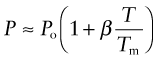
where P is the value of the property, Po its low-temperature value and β is a constant. Figure 13.1 shows four examples: density, modulus, refractive index and—for metals—electrical resistivity. Thus, the density ρ and refractive index n decrease by about 6% on heating from cold to the melting point Tm(β ≈ −0.06), the modulus E falls by a factor of 2 (β ≈ −0.5), and the resistivity R increases by a factor of about 7 (β ≈ +6). These changes cannot be neglected, but are easily accommodated by using the value of the property at the temperature of the design.
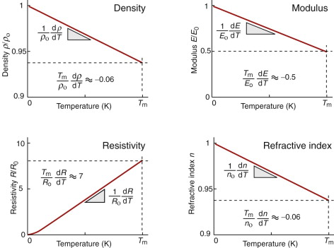
Figure 13.1 Linear dependence of properties on temperature: density, modulus, resistivity and refractive index.
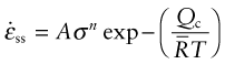
Other properties are less forgiving. Strength falls in a much more sudden way and the rate of creep—the main topic here—increases exponentially (Figure 13.2). This we need to explore in more detail.
Viscous flow
When a substance flows, its particles change neighbours; flow is a process of shear. Newton’s law describes the flow rate in fluids under a shear stress τ:

where ![]() is the shear rate and η the viscosity (units Pa.s). This is a linear law, like Hooke’s law, with the modulus replaced by the viscosity and the strain by strain rate (units s−1). Viscous flow occurs at constant volume (Poisson’s ratio = 0.5) and this means that problems of viscous flow can be solved by taking the solution for elastic deformation and replacing the strain ε by the strain rate
is the shear rate and η the viscosity (units Pa.s). This is a linear law, like Hooke’s law, with the modulus replaced by the viscosity and the strain by strain rate (units s−1). Viscous flow occurs at constant volume (Poisson’s ratio = 0.5) and this means that problems of viscous flow can be solved by taking the solution for elastic deformation and replacing the strain ε by the strain rate ![]() and, using equation (4.10), Young’s modulus E by 3η. Thus, the rate at which a rod of a very viscous fluid, like tar, extends when pulled in tension is
and, using equation (4.10), Young’s modulus E by 3η. Thus, the rate at which a rod of a very viscous fluid, like tar, extends when pulled in tension is

The factor 1/3 appears because of the conversion from shear to normal stress and strain.
Example 13.1
A tar has a viscosity of η = 108 Pa.s. A cube of tar with a cross-section of A = 0.01 mm2 is placed under a steel plate with a mass m of 0.5 kg. By how much will the cube shorten in 1 day?
Answer. The stress σ = mg/A = 490 MPa. The compressive strain-rate is ![]() . The compressive strain in 1 day (t = 8.64 × 10⁴ s) is thus
. The compressive strain in 1 day (t = 8.64 × 10⁴ s) is thus ![]() . The initial edge length of the cube is 100 mm, so it will shorten by 13.8 mm.
. The initial edge length of the cube is 100 mm, so it will shorten by 13.8 mm.
Creep
At room temperature, most metals and ceramics deform in a way that depends on stress but not on time. As the temperature is raised, loads that are too small to give permanent deformation at room temperature cause materials to creep: to undergo slow, continuous deformation with time, ending in fracture. It is usual to refer to the time-independent behaviour as ‘low-temperature’ response, and the time-dependent flow as ‘high-temperature’ response. But what, in this context, is ‘low’ and what is ‘high’? The melting point of tungsten, used for lamp filaments, is over 3000 °C. Room temperature, for tungsten, is a very low temperature. The filament temperature in a tungsten lamp is about 2000 °C. This, for tungsten, is a high temperature: the filament slowly sags over time under its own weight until the turns of the coil touch and the lamp burns out.
To design against creep we need to know how the strain rate ![]() or time to failure tf depends on the stress σ and temperature T to which it is exposed. That requires creep testing.
or time to failure tf depends on the stress σ and temperature T to which it is exposed. That requires creep testing.
Creep testing and creep curves
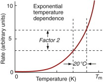
Creep is measured in the way shown in Figure 13.3. A specimen is loaded in tension or compression, usually at constant load, inside a furnace that is maintained at a constant temperature, T. The extension is measured as a function of time. Metals, polymers and ceramics all have creep curves with the general shape shown in the figure.
Figure 13.3 Creep testing and the creep curve, showing how strain ε increases with time t up to the fracture time tf.
The initial elastic and the primary creep strains occur quickly and can be treated in much the way that elastic deflection is allowed for in a structure. Thereafter, the strain increases steadily with time in what is called the secondary creep or the steady-state creep regime. Plotting the log of the steady-state creep rate, ![]() , against the log of the stress, σ, at constant T, as in Figure 13.4(a), shows that
, against the log of the stress, σ, at constant T, as in Figure 13.4(a), shows that
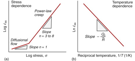
where n, the creep exponent, usually lies between 3 and 8, and for that reason this behaviour is called power-law creep. At low σ there is a tail with slope n ≈ 1 (the part of the curve labeled ‘Diffusional flow’ in Figure 13.4(a)). By plotting the natural logarithm (ln) of ![]() against the reciprocal of the absolute temperature (1/T) at constant stress, as in Figure 13.4(b), we find that:
against the reciprocal of the absolute temperature (1/T) at constant stress, as in Figure 13.4(b), we find that:
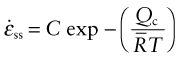
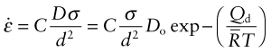
Here ![]() is the gas constant (8.31 J/mol/K) and Qc is called the activation energy for creep, with units of J/mol. The creep rate
is the gas constant (8.31 J/mol/K) and Qc is called the activation energy for creep, with units of J/mol. The creep rate ![]() increases exponentially in the way suggested by Figure 13.2; increasing the temperature by as little as 20 °C can double the creep rate. Combining these two findings gives
increases exponentially in the way suggested by Figure 13.2; increasing the temperature by as little as 20 °C can double the creep rate. Combining these two findings gives
where C′ is a constant. Written in this way the constant C′ has weird units (s−1 · MPa−n) so it is more usual and sensible to write instead
The four constants ![]() (units: s−1), σo (units: MPa), n and Qc characterise the steady state creep of a material; if you know these, you can calculate the strain rate
(units: s−1), σo (units: MPa), n and Qc characterise the steady state creep of a material; if you know these, you can calculate the strain rate ![]() at any temperature and stress using equation (13.6). They vary from material to material and have to be measured experimentally. We meet values for them in Section 13.5.
at any temperature and stress using equation (13.6). They vary from material to material and have to be measured experimentally. We meet values for them in Section 13.5.
Sometimes creep is desirable. Extrusion, hot rolling, hot pressing and forging are carried out at temperatures at which power-law creep is the dominant mechanism of deformation; exploiting it reduces the pressure required for the operation. The change in forming pressure for a given change in temperature can be calculated from equation (13.6).
Example 13.2
A stainless steel tie of length L = 100 mm is loaded in tension under a stress σ = 150 MPa at a temperature T = 800 °C. The creep constants for stainless steel are: reference strain-rate ![]() , reference stress σo = 100 MPa, stress exponent n = 7.5 and activation energy for power-law creep Qc = 280 kJ/mol. What is the creep rate of the tie? By how much will it extend in 100 hours?
, reference stress σo = 100 MPa, stress exponent n = 7.5 and activation energy for power-law creep Qc = 280 kJ/mol. What is the creep rate of the tie? By how much will it extend in 100 hours?
Answer. The steady state creep rate is given by ![]() . Using the data listed above, converting the temperature to Kelvin, and using the gas constant
. Using the data listed above, converting the temperature to Kelvin, and using the gas constant ![]() gives
gives ![]() . After 100 hours (3.6 × 10⁵ seconds) the strain is ε = 0.173 and the 100 mm long tie has extended by ΔL = 17.3 mm.
. After 100 hours (3.6 × 10⁵ seconds) the strain is ε = 0.173 and the 100 mm long tie has extended by ΔL = 17.3 mm.
Creep damage and creep fracture
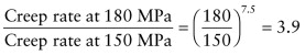
As creep continues, damage accumulates. It takes the form of voids or internal cracks that slowly expand and link, eating away the cross-section and causing the stress to rise. This makes the creep rate accelerate as shown in the tertiary stage of the creep curve of Figure 13.3. Since ![]() with n ≈ 5, the creep rate goes up even faster than the stress: an increase of stress of 10% gives an increase in creep rate of 60%.
with n ≈ 5, the creep rate goes up even faster than the stress: an increase of stress of 10% gives an increase in creep rate of 60%.
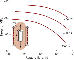
Times to failure, tf, are normally presented as creep–rupture diagrams (Figure 13.5). Their application is obvious: if you know the stress and temperature you can read off the life. If instead you wish to design for a certain life at a certain temperature, you can read off the design stress. Experiments show that
which is called the Monkman–Grant law. The Monkman–Grant constant, C, is typically 0.05–0.3. Knowing it, the creep life (meaning tf) can be estimated from equation (13.6).
Example 13.3
A component in a chemical engineering plant is made of the stainless steel of Example 13.2. It is loaded by an internal pressure that generates a hoop stress of 150 MPa. (a) If the hoop creep-rate ![]() at T = 800 °C under this stress, by what factor will it increase if the pressure is raised by 20%? (b) If instead the pressure is held constant but the temperature is raised from T1 = 800 °C to T2 = 850 °C, by what factor will the creep life tf be reduced?
at T = 800 °C under this stress, by what factor will it increase if the pressure is raised by 20%? (b) If instead the pressure is held constant but the temperature is raised from T1 = 800 °C to T2 = 850 °C, by what factor will the creep life tf be reduced?
Answer. (a) The hoop stress is proportional to the pressure. Thus the factor by which the strain rate increases when the pressure is raised is
 ; the creep rate increases to
 (b) The factor by which the strain rate is increased by the increase in temperature is
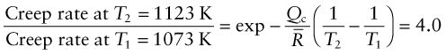
The creep life ![]() where C is a constant. The creep life therefore is reduced by the same factor. The message here is that comparatively small changes in stress or temperature cause big changes in creep rate and creep life because of their strongly nonlinear dependence on both σ and T.
where C is a constant. The creep life therefore is reduced by the same factor. The message here is that comparatively small changes in stress or temperature cause big changes in creep rate and creep life because of their strongly nonlinear dependence on both σ and T.
13.3 Charts for creep behaviour
Melting point
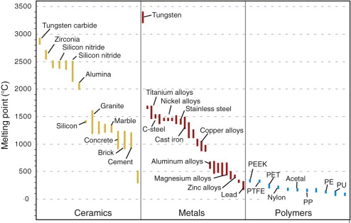
Figure 13.6 shows melting points for metals, ceramics and polymers. Most metals and ceramics have high melting points and, because of this, they start to creep only at temperatures well above room temperature. Lead, however, has a melting point of 327 °C (600 K), so room temperature is almost half its absolute melting point and it creeps—a problem with lead roofs and cladding of old buildings. Crystalline polymers, most with melting points in the range 150–200 °C, creep slowly if loaded at room temperature; glassy polymers, with Tg of typically 50–150 °C, do the same. The point, then, is that the temperature at which materials start to creep depends on their melting points. As a general rule, it is found that creep starts when T ≈ 0.35 Tm for metals and 0.45 Tm for ceramics, although alloying can raise this temperature significantly.
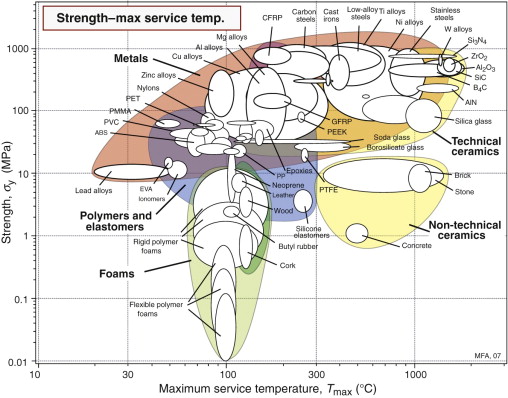
Maximum service temperature and strength
Figure 13.7 charts the maximum service temperature Tmax and room temperature strength σy. It shows that polymers and low melting metals like the alloys of zinc, magnesium and aluminum offer useful strength at room temperature but by 300 °C they cease to be useful—indeed, few polymers have useful strength above 135 °C. Titanium alloys and low-alloy steels have useful strength up to 600 °C; above this temperature high-alloy stainless steels and more complex alloys based on nickel, iron and cobalt are needed. The highest temperatures require refractory metals like tungsten or technical ceramics such as silicon carbide (SiC) or alumina (Al2O3).
Creep strength at 950 °C and density
Figure 13.8 is an example of a chart to guide selection of materials for load-bearing structures that will be exposed to high temperatures. It shows the creep strength at 950 °C, σ950°C. Strength at high temperatures (and this is a very high temperature), as we have said, is rate dependent, so to construct the chart we first have to choose an acceptable strain rate, one we can live with. Here 10−6/s has been chosen. σ950°C is plotted against the density ρ. The chart is used in exactly the same way as the σy−ρ chart of Figure 6.6, allowing indices like
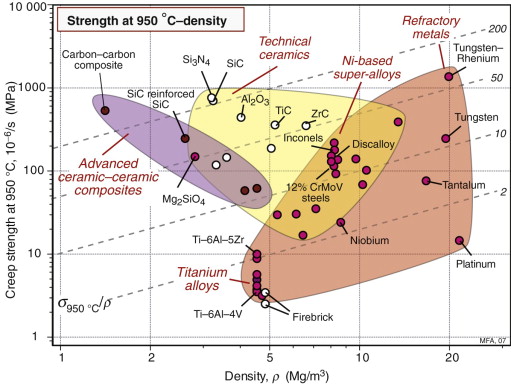
Figure 13.8 A chart showing the strength of selected materials at a particularly high temperature—950 °C and a strain rate of 10−6/s—plotted against density. Software allows charts like this to be constructed for any chosen temperature. (The chart was made with a specialised high-temperature materials database that runs in the CES system.)
to be plotted to identify materials for lightweight design at high temperature. Several such contours are shown.
The figure shows that titanium alloys, at this temperature, have strengths of only a few megapascals—about the same as lead at room temperature. Nickel- and iron-based super-alloys have useful strengths of 100 MPa or more. Only refractory metals like alloys of tungsten, technical ceramics like SiC and advanced (and very expensive) ceramic–ceramic composites offer high strength.
At room temperature we need only one strength–density chart. For high-temperature design we need one that is constructed for the temperature and acceptable strain rate or life required by the design. It is here that computer-aided methods become particularly valuable, because they allow charts like Figure 13.8 to be constructed and manipulated for any desired set of operating conditions quickly and efficiently.
13.4 The science: diffusion and creep
Viscous flow and creep require the relative motion of atoms. How does this happen, and what is its rate? Think first of the unit step—one atom changing its position relative to those around it by what is called diffusion.
Diffusion
Diffusion is the spontaneous intermixing of atoms over time. In gases and liquids intermixing is familiar—the dispersion of smoke in still air, the dispersion of an ink drop in water—and understood as the random motion of the atoms or molecules (Brownian motion). But in crystalline solids atoms are confined to lattice sites—how then are they going to mix? In practice they do. If atoms of type A are plated onto a block of atoms of type B and the A–B couple is heated, the atoms interdiffuse at a rate described by Fick’s law1:
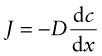
Here J is the atom flux (the number of atoms of type A diffusing across unit area of surface per second), D is the diffusion coefficient and dc/dx is the gradient in concentration c of A atoms in the x direction.
Heat, as we have said, is atoms in motion. In a solid they vibrate about their mean position with a frequency ν (about 1013 per second) with an average energy, kinetic plus potential, of kBT in each mode of vibration, where kB is Boltzmann’s constant (1.38 × 10⁻²³ J/atom · K). This is the average, but at any instant some atoms have less, some more. Statistical mechanics gives the distribution of energies. The Maxwell–Boltzmann equation describes the probability p that a given atom has an energy greater than a value q Joules:
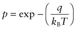
Crystals, as said in Chapter 4, contain vacancies—occasional empty atom sites. These provide a way for diffusive jumps to take place. Figure 13.9 shows an atom jumping into a vacancy. To make such a jump, the atom marked in red (though it is the same sort of atom as the rest) must break away from its original comfortable site at A, its ground state, and squeeze between neighbors, passing through an activated state, to drop into the vacant site at B where it is once again comfortable. There is an energy barrier, qm, between the ground state and the activated state to overcome if the atom is to move. The probability pm that a given atom has thermal energy this large or larger is just equation (13.9) with q = qm.
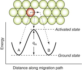
Figure 13.9 A diffusive jump. The energy graph shows how the energy of the red atom (which may be chemically the same as the green ones, or may not) changes as it jumps from site A to site B.
So two things are needed for an atom to switch sites: enough thermal energy and an adjacent vacancy. A vacancy has an energy qv, so—not surprisingly—the probability pv that a given site be vacant is also given by equation (13.9), this time with q = qv. Thus, the overall probability of an atom changing sites is
where qd is called the activation energy for self-diffusion. If instead the red atom were chemically different from the green ones (so it is in solid solution), the process is known as interdiffusion. Its activation energy has the same origin.
Figure 13.10 illustrates how mixing occurs by interdiffusion. It shows a solid in which there is a concentration gradient dc/dx of red atoms: there are more in slice A immediately to the left of the central, shaded plane, than in slice B to its right. If atoms jump across this plane at random there will be a net flux of red atoms to the right because there are more on the left to jump, and a net flux of white atoms in the opposite direction. The number of red atoms in slice A, per unit area, is nA = 2rocA and that in slice B is nB = 2rocB, where 2ro, the atom size, is the thickness of the slices, and cA and cB are the concentration of red atoms on the two planes expressed as atom fractions. The difference is
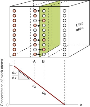
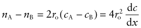
(since cA − cB = 2ro(dc/dx)). The number of times per second that an atom on slice A oscillates toward B, or one on B toward A, is ν/6, since there are six possible directions in which an atom can oscillate in three dimensions, only one of which is in the right direction. Thus, the net flux of red atoms from left to right is
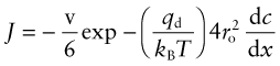
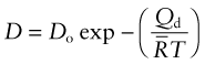
It is usual to list the activation energy per mole, Qd, rather than that per atom, qd, so we write Qd = NAqd and ![]() = NAkB (where NA is Avogadro’s number, 6.02 × 10²³), and assemble the terms 4νr2o/6 into a single constant Do to give
= NAkB (where NA is Avogadro’s number, 6.02 × 10²³), and assemble the terms 4νr2o/6 into a single constant Do to give
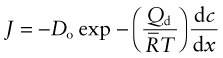
which has the form of Fick’s law (equation (13.8)) with the diffusion coefficient D given by
(The CES Elements database contains data for Do and Qd for the elements.)
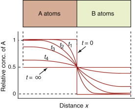
Fourier’s law for heat flow (equation (12.2)) and Fick’s law for the flow of matter (equation (13.8)) have identical forms. This means solutions to problems of heat flow are the same as those for matter flow if a is replaced by D and dT/dx is replaced by dc/dx. This includes solutions to transient problems. Figure 13.11 shows successive concentration profiles at times t1, t2, t3, t4 as red atoms on the left and green atoms on the right interdiffuse. This is a transient matter flow problem. Just as with transient heat flow (equation (12.15)), the mean distance x that one type of atom has penetrated the other is given by
There are two further rules of thumb, useful in making estimates of diffusion rates when data are not available and to give a feel for the upper limit for diffusion rate. The first is that the activation energy for diffusion, normalised by ![]() , is approximately constant for metals:
, is approximately constant for metals:

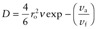
The second is that the diffusion coefficient of metals, evaluated at their melting point, is also approximately constant:

Example 13.4
Alumina, Al2O3 is suggested for the membrane of a fuel cell. To assess the performance of the cell for oxygen ion transport, the diffusion coefficient of oxygen ions in the membrane at the maximum practical operating temperature T = 1100 °C is needed. If it is less than D = 10−12 m2/s the cell is impractical. The activation energy of oxygen diffusion in Al2O3 is Qd = 636 kJ/mol and the pre-exponential factor is Do = 0.19 m2/s. Will the cell work?
Answer. The oxygen diffusion coefficient at T = 1100 °C is

Example 13.5
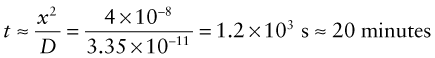
It is proposed to harden a low carbon steel component to a depth x = 0.2 mm by diffusing carbon into the surface from a carbon pack at T = 1100 °C. The diffusion constants for carbon in austenitic iron (the stable phase at 1000 °C) are Do = 8 × 10⁻⁶ m2/s and Qd = 131 kJ/mol. For how long must the component be cooked to achieve the desired depth of hardening?
Answer. The diffusion coefficient at 1000 °C is ![]()
The time to diffuse a distance x = 0.2 mm is approximately
Diffusion in liquids and non-crystalline solids
The vacancies in a crystal can be thought of as free volume—free because it is able to move, as it does when an atom jumps. The free volume in a crystal is thus in the form of discrete units, all of the same size—a size into which an atom with enough thermal energy can jump. Liquids and non-crystalline solids, too, contain free volume, but because there is no lattice or regular structure it is dispersed randomly between all the atoms or molecules. Experiments show that the energy barrier to atom movement in liquids is not the main obstacle to diffusion or flow. There is actually plenty of free volume among neighbors of any given particle, but it is of little use for particle jumps except when, by chance, it comes together to make an atom-sized hole—a temporary vacancy. This is a fluctuation problem just like that of the Maxwell–Boltzmann problem, but a fluctuation of free volume rather than thermal energy, and with a rather similar solution: diffusion in liquids is described by
where vf is the average free volume per particle, va is the volume of the temporary vacancy, and ro and v have the same meaning as before.
Diffusion driven by other fields
So far we have thought of diffusion driven by a concentration gradient. Concentration c is a field quantity; it has discrete values at different points in space (the concentration field). The difference in c between two nearby points divided by the distance between them defines the local concentration gradient, dc/dx.
Diffusion can be driven by other field gradients. A stress gradient, as we shall see in a moment, drives diffusional flow and power-law creep. An electric field gradient can drive diffusion in nonconducting materials. Even a temperature gradient can drive diffusion of matter as well as diffusion of heat.
Diffusional flow
Liquids and hot glasses are wobbly structures, a bit like a bag loosely filled with beans. If atoms (or beans) move inside the structure, the shape of the whole structure changes in response. Where there is enough free volume, a stress favors the movements that change the shape in the direction of the stress, and opposes those that do the opposite, giving viscous flow. The higher the temperature, the more is the free volume and the faster the flow.
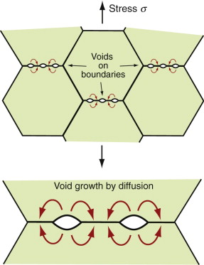
But how do jumping atoms change the shape of a crystal? A crystal is not like a bag of loose beans—the atoms have well-defined sites on which they sit. In the cluster of atoms in Figure 13.9 an atom has jumped but the shape of the cluster has not changed. At first sight, then, diffusion will not change the shape of a crystal. In fact it does, provided the material is polycrystalline—made up of many crystals meeting at grain boundaries. This is because the grain boundaries act as sources and sinks for vacancies. If a vacancy joins a boundary, an atom must leave it; repeat this many times and that face of the crystal is eaten away. If instead a vacancy leaves a boundary, an atom must join it and—repeated—that face grows. Figure 13.12 shows the consequences: the slow extension of the polycrystal in the direction of stress. It is driven by a stress gradient: the difference between the tensile stress σ on the horizontal boundaries from which vacancies flow and that on the others, essentially zero, to which they go. If the grain size is d the stress gradient is σ/d. The flux of atoms, and thus the rate at which each grain extends, δd/δt, is proportional to Dσ/d. The strain rate, ![]() , is the extension rate divided by the original grain size, d, giving
, is the extension rate divided by the original grain size, d, giving
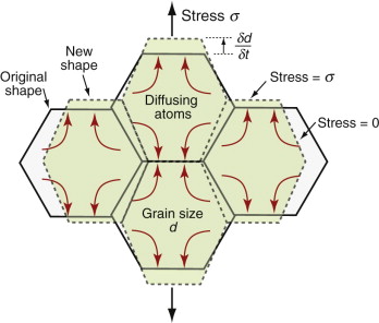
where C is a constant. This is a sort of viscous flow, linear in stress. The smaller the grain size, the faster it goes.
Dislocation climb and power-law creep
Plastic flow, as we saw in Chapter 5, is the result of the motion of dislocations. Their movement is resisted by dissolved solute atoms, precipitate particles, grain boundaries and other dislocations; the yield strength is the stress needed to force dislocations past or between them. Diffusion can unlock dislocations from obstacles in their path, making it easier for them to move. Figure 13.13 shows how it happens. Here a dislocation is obstructed by a particle. The glide force τb per unit length is balanced by the reaction fo from the precipitate. But if the atoms of the extra half-plane diffuse away, thus eating a slot into the half-plane, the dislocation can continue to glide even though it now has a step in it. The stress gradient this time is less obvious—it is the difference between the local stress where the dislocation is pressed against the particle and that on the dislocation remote from it. The process is called ‘climb’ and, since it requires diffusion, it can occur at a measurable rate only when the temperature is above about 0.35TM.
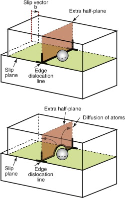
Figure 13.13 Climb of a dislocation: the extra half-plane is eaten away by diffusion, allowing the dislocation to pass the obstacle. The result is power-law creep.
Climb unlocks dislocations from the obstacles that pin them, allowing further slip. After a little slip, of course, the unlocked dislocations encounter the next obstacles, and the whole cycle repeats itself. This explains the progressive, continuous, nature of creep. The dependence on diffusion explains the dependence of creep rate on temperature, with
with Qc ≈ Qd. The power-law dependence on stress σ is harder to explain. It arises partly because the stress gradient driving diffusion increases with σ and partly because the density of dislocations itself increases too.
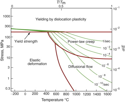
Deformation mechanism diagrams
Let us now pull all this together. Materials can deform by dislocation plasticity (Chapter 6) or, if the temperature is high enough, by diffusional flow or power-law creep. If the stress and temperature are too low for any of these, the deformation is elastic. This competition between mechanisms is summarised in deformation mechanism diagrams, of which Figure 13.14 is an example. It shows the range of stress and temperature in which we expect to find each sort of deformation and the strain rate that any combination of them produces (the contours). Diagrams like these are available for many metals and ceramics, and are a useful summary of creep behaviour, helpful in selecting a material for high-temperature applications—one appears in the examples at the end of this chapter.
Creep fracture
Diffusion, we have seen, gives creep. It also gives creep fracture. You might think that a creeping material would behave like toffee or chewing gum—that it would stretch a long way before breaking in two—but for crystalline materials this is very rare. Indeed, creep fracture (in tension) can happen at unexpectedly small strains, often only 2–5%, by the mechanism shown in Figure 13.15. Voids nucleate on grain boundaries that lie normal to the tensile stress. These are the boundaries to which atoms diffuse to give diffusional creep, coming from the boundaries that lie more nearly parallel to the stress. But if the tensile boundaries have voids on them, they act as sources of atoms too, and in doing so, they grow. The voids cannot support load, so the stress rises on the remaining intact bits of boundary, making the voids grow more and more quickly until finally (bang) they link.
Many engineering components (e.g. tie-bars in furnaces, super-heater tubes, high-temperature pressure vessels in chemical reaction plants) are expected to withstand moderate creep loads for long times (say 20 years) without failure. The loads or pressure they can safely carry are calculated by methods such as those we have just described. We would like to be able to test new materials for these applications without having to wait 20 years for the results. It is thus tempting to speed up the tests by increasing the load or the temperature to get observable creep in a short test time, and this is done. But there are risks. Tests carried out on the steep n = 3–8 branch of Figure 13.4(a), if extrapolated to lower stresses where n ≈ 1, greatly underestimate the creep rate.
Creep mechanisms: polymers
Creep in crystalline materials, as we have seen, is closely related to diffusion. The same is true of polymers, but because most of them are partly or wholly amorphous, diffusion is controlled by free volume (equation (13.14)). Free volume increases with temperature (its fractional change per degree is just the volumetric thermal expansion, 3α) and it does so most rapidly at the glass transition temperature Tg. Thus, polymers start to creep as the temperature approaches Tg and that, for most, is a low temperature: 50–150 °C.
This means that the temperature range in which most polymers are used is that near Tg when they are neither simple elastic solids nor viscous liquids; they are visco-elastic solids. If we represent the elastic behaviour by a spring and the viscous behaviour by a dash-pot, then visco-elasticity (at its simplest) is described by a coupled spring and dash-pot as in Figure 13.16. Applying a load causes creep, but at an ever-decreasing rate because the spring takes up the tension. Releasing the load allows slow reverse creep, caused by the extended spring.
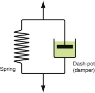
Figure 13.16 Visco-elastic behaviour can be modeled as a spring (the elastic part) in parallel with a dash-pot (the viscous part).
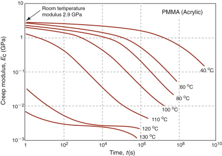
Real polymers require more elaborate systems of springs and dash-pots to describe them. This approach of polymer rheology can be developed to provide criteria for design, but these are complex. A simpler approach is to use graphical data for what is called the creep modulus, Ec, to provide an estimate of the deformation during the life of the structure. Figure 13.17 shows data for Ec as a function of temperature T and time t. Creep modulus data allow elastic solutions to be used for design against creep. The service temperature and design life are chosen, the resulting creep modulus is read from the graph, and this is used instead of Young’s modulus in any of the solutions to design problems listed in Chapter 5.
13.5 Materials to resist creep
Metals and ceramics to resist creep
Diffusional flow is important when grains are small (as they often are in ceramics) and when the component is subject to high temperatures at low loads. Equation (13.15) says that the way to avoid diffusional flow is to choose a material with a high melting temperature and arrange that it has a large grain size, d, so that diffusion distances are long. Single crystals are best of all; they have no grain boundaries to act as sinks and sources for vacancies, so diffusional creep is suppressed completely. This is the rationale behind the wide use of single-crystal turbine blades in jet engines.
That still leaves power-law creep. Materials that best resist power-law creep are those with high melting points, since diffusion and thus creep rates scale as T/Tm, and a microstructure that maximises obstruction to dislocation motion through alloying to give a solid solution and precipitate particles. Current creep-resistant materials, known as super-alloys, are remarkably successful in this. Most are based on iron, nickel or cobalt, heavily alloyed with aluminum, chromium and tungsten. The chart of Figure 13.8 shows both effects: the high melting point refractory metals and the heavily alloyed super-alloys.
Many ceramics have high melting points, meeting the first criterion. They do not need alloying because their covalent bonding gives them a large lattice resistance. Typical among them are the technical ceramics alumina (Al2O3), silicon carbide (SiC) and silicon nitride (Si3N4)—they too appear in Figure 13.8. The lattice resistance pins down dislocations but it also gives the materials low fracture toughness, even at high temperature, making design to use them difficult.
Polymers to resist creep
The creep resistance of polymers scales with their glass temperature. Tg increases with the degree of cross-linking; heavily cross-linked polymers (e.g. epoxies) with high Tg are therefore more creep resistant at room temperature than those that are not (like polyethylene). The viscosity of polymers above Tg increases with molecular weight, so the rate of creep is reduced by having a high molecular weight. Finally, crystalline or partly crystalline polymers (e.g. high-density polyethylene) are more creep resistant than those that are entirely glassy (e.g. low-density polyethylene).
The creep rate of polymers is reduced by filling them with powdered glass, silica (sand) or talc, roughly in proportion to the amount of filler. PTFE on saucepans and polypropylene used for automobile components are both strengthened in this way. Much better creep resistance is obtained with composites containing chopped or continuous fibres (GFRP and CFRP), because much of the load is now carried by the fibres that, being very strong, do not creep at all.
Selecting materials to resist creep
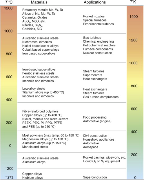
Classes of industrial applications tend to be associated with certain characteristic temperature ranges. There is the cryogenic range, between −273 °C and roughly room temperature, associated with the use of liquid gases like hydrogen, oxygen or nitrogen. Here the issue is not creep, but the avoidance of brittle fracture. There is the regime at and near room temperature (−20 to +150 °C) associated with conventional mechanical and civil engineering: household appliances, sporting goods, aircraft structures and housing are examples. Above this is the range 150–400 °C, associated with automobile engines and with food and industrial processing. Higher still are the regimes of steam turbines and superheaters (typically 400–650 °C), and of gas turbines and chemical reactors (650–1000 °C). Special applications (lamp filaments, rocket nozzles) require materials that withstand even higher temperatures, extending as high as 2800 °C.
Materials have evolved to fill the needs of each of these temperature ranges (Figure 13.18). Certain polymers, and composites based on them, can be used in applications up to 250 °C, and now compete with magnesium and aluminum alloys and with the much heavier cast irons and steels, traditionally used in those ranges. Temperatures above 400 °C require special creep-resistant alloys: ferritic steels, titanium alloys (lighter, but more expensive) and certain stainless steels. Stainless steels and ferrous super-alloys really come into their own in the temperature range above this, where they are widely used in steam turbines and heat exchangers. Gas turbines require, in general, nickel-based or cobalt-based super-alloys. Above 1000 °C, the refractory metals and ceramics become the only candidates. Materials used at high temperatures will, generally, perform perfectly well at lower temperatures too, but are not used there because of cost.
The chart of Figure 13.8 showed the performance of materials able to support load at 950 °C. Charts like this are used in design in the same way as those for low-temperature properties.
13.6 Design to cope with creep
Creep problems are of four types:
- Those in which limited creep strain can be accepted but creep rupture must be avoided, as in the creep of pipework or of lead roofs and cladding on buildings.
- Those in which creep strain is design limiting, as it is for blades in steam and gas turbines where clearances are critical.
- Those involving more complex problems of creep strain, loss of stiffness and risk of buckling—a potential problem with space-frames of supersonic aircraft and space vehicles.
- Those involving stress relaxation—the loss of tension in a pre-tightened bolt, for instance.
Predicting life of high-temperature pipework
Chemical engineering and power generation plants have pipework that carries hot gases and liquids under high pressure. A little creep, expanding the pipe slightly, can be accepted; rupture, with violent release of hot, high-pressure fluid, cannot. We take, as an example, pipework in a steam-turbine power-generating station. Pipes in a typical 600 MW unit carry steam at 650 °C and a pressure p of 15 MPa. The stress in the wall of a thin-walled pipe with a radius R and a wall thickness t carrying a pressure p, as in Figure 13.19, is
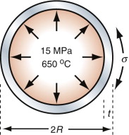

Suppose you have been asked to recommend a pipe required as a temporary fix while modifications are made to the plant. Space is constrained: the pipe cannot be more than 300 mm in diameter. The design life is six months. A little creep does not matter, but the pipe must not rupture. Type 304 stainless steel pipe with a diameter of 300 mm and a wall thickness of 10 mm is available. Will it function safely for the design life?
The stress in the pipe wall with these dimensions, from equation (13.17), is 225 MPa. Figure 13.20 shows stress–rupture data for Type 304 stainless steel. Enter 225 MPa at 650 °C and read off the rupture life: about seven hours. Not so good.
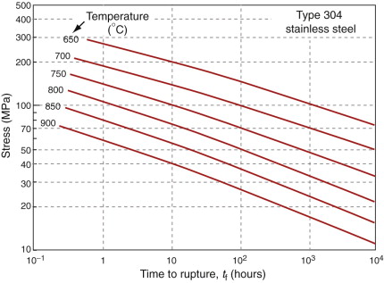
So how thick should the pipe be? To find out, reverse the reasoning. The design life is six months—4380 hours. A safety-critical component such as this one needs a safety factor, so double it: 8760 hours. Enter this and the temperature on the stress–rupture plot and read off the acceptable stress: 80 MPa. Put this into equation (13.17) to calculate the wall thickness. To be safe the pipe wall must be at least 28 mm thick.
Turbine blades
Throughout the history of its development, the gas turbine has been limited in thrust and efficiency by the availability of materials that can withstand high stress at high temperatures. The origin of the stress is the centrifugal load carried by the rapidly spinning turbine disk and rotor blades. Where conditions are at their most extreme, in the first stage of the turbine, nickel- and cobalt-based super-alloys currently are used because of their unique combination of high-temperature strength, toughness and oxidation resistance. Typical of these is MAR-M200, an alloy based on nickel, strengthened by a solid solution of tungsten and cobalt and by precipitates of Ni3(Ti,A1), and containing chromium to improve its resistance to attack by gases.
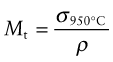
When a turbine is running at a steady speed, centrifugal forces subject each rotor blade to an axial tension (equation (7.8)). If the blade has a constant cross-section, the tensile stress rises linearly from zero at its tip to a maximum at its root. As an example, a rotor of radius r = 0.3 m rotating at an angular velocity ω of 10 000 rpm (1000 radians/s) induces an axial stress (Rω2ρx) of order 150 MPa. (Here ρ is the density of the alloy, about 8000 kg/m3, and x the distance from the tip; a typical blade is about 80 mm long.) Typical stress and temperature profiles for a blade in a medium-duty engine are shown in Figure 13.21. They are plotted as a shaded box onto two deformation mechanism maps in Figure 13.22. If made of pure nickel (Figure 13.22(a)) the blade would deform by power-law creep, at a totally unacceptable rate. The strengthening methods used in MAR-M200 with a typical as-cast grain size of 0.1 mm (Figure 13.22(b)) reduce the rate of power-law creep by a factor of 106 and change the dominant mechanism of flow from power-law creep to diffusional flow. Further solution strengthening or precipitation hardening is now ineffective unless it slows this mechanism. A new strengthening method is needed: the obvious one is to increase the grain size or remove grain boundaries altogether by using a single crystal. This slows diffusional flow or stops it altogether, while leaving the other flow mechanisms unchanged. The power-law creep field expands and the rate of creep of the turbine blade falls to a negligible level.
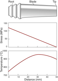
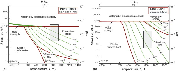
Figure 13.22 (a) The stress–temperature profile of the blade plotted onto a deformation map for pure nickel. (b) The same profile plotted on a map for the alloy MAR-M200. The strain rates differ by a factor of almost 106.
The point to remember is that creep has contributions from several distinct mechanisms; the one that is dominant depends on the stress and temperature applied to the material. If one is suppressed, another will take its place. Strengthening methods are selective: a method that works well in one range of stress and temperature may be ineffective in another. A strengthening method should be regarded as a way of attacking a particular flow mechanism. Materials with good creep resistance combine strengthening mechanisms in order to attack them all; single-crystal MAR-M200 is a good example of this.
Thermal barrier coatings
The efficiency and power-to-weight ratio of advanced gas turbines, as already said, is limited by the burn temperature and this in turn is limited by the materials of which the rotor and stator blades are made. Heat enters the blade from the burning gas, as shown in Figure 13.23. Blades are cooled by pumping air through internal channels, leading to the temperature profile shown on the left. The surface temperature of the blade is set by a balance between the heat transfer coefficient between gas and blade (determining the heat in) and conduction within the blade to the cooling channel (determining the heat out). The temperature step at the surface is increased by bleeding a trickle of the cooling air through holes in the blade surface. This technology is already quite remarkable—air-cooled blades operate in a gas stream at a temperature that is above the melting point of the alloy of which they are made. How could the burn temperature be increased yet further?
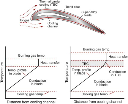
Figure 13.23 A cross-section of a turbine blade with a thermal barrier coating (TBC). The temperature profile for the uncoated blade is shown on the left, that for the coated blade on the right.
Many ceramics have higher melting points than any metal and some have low thermal conductivity. Ceramics are not tough enough to make the whole blade, but coating the metal blade with a ceramic to form a thermal barrier coating (TBC) allows an increase in gas temperature with no increase in that of the blade, as shown on the right. How is the ceramic chosen? The first considerations are those of a low thermal conductivity, a maximum service temperature above that of the gas (providing some safety margin) and adequate strength. The α−λ chart (Figure 12.4) shows that the technical ceramic with by far the lowest thermal conductivity is zirconia (ZrO2). The Tmax−σf chart (Figure 13.7) confirms that it is usable up to very high temperature and has considerable strength. Zirconia looks like a good bet—and indeed it is this ceramic that is used for TBCs.
As always, it is not quite so simple. Other problems must be overcome to make a good TBC. It must stick to the blade, and that is not easy. To achieve it the blade surface is first plated with a thin bond coat (a complex Ni–Cr–Al–Y alloy); it is the glue, so to speak, between blade and coating, shown in Figure 13.23. Most ceramics have a lower expansion coefficient than the super-alloy of the blade (compare α for ZrO2 and Ni in Figure 12.4) so when the blade heats up it expands more than the coating and we know what that means: thermal stresses and cracking. The problem is solved (amazingly) by arranging that the coating is already cracked on a fine scale, with all the cracks running perpendicular to its surface, making an array of interlocking columns like a microscopic Giant’s Causeway. When the blade expands the columns separate very slightly, but not enough for hot gas to penetrate to any significant extent; its protective thermal qualities remain. Next time you fly, reflect on all this—the plane you are in almost certainly has coated blades.
Airframes
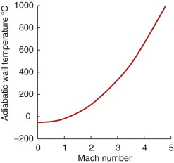
If you want to fly at speeds above Mach 1 (760 mph), aerodynamic heating becomes a problem. It is easiest to think of a static structure in a wind tunnel with a supersonic air stream flowing over it. In the boundary layer immediately adjacent to the structure, the velocity of the air is reduced to zero and its kinetic energy appears as heat, much of which is dumped into the skin of the structure. The surface temperature Ts can be calculated; it is approximately
Here Ma is the Mach number and To the ambient temperature. Supersonic flight is usually at altitudes above 35 000 ft, where To = −50 °C. Figure 13.24 shows what Ts looks like.
This, not surprisingly, causes problems. First, creep causes a gradual change in dimension over time; wing deflection can increase, affecting aerodynamic performance. Second, thermal stress caused by expansion can lead to further creep damage because it adds to aerodynamic loads. Finally, the drop in modulus, E, brings greater elastic deflection and changes the buckling and flutter (meaning vibration) characteristics.
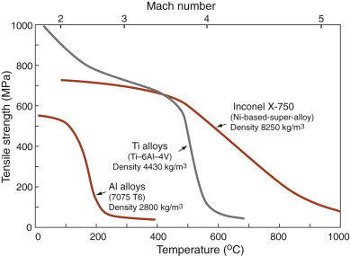
In a large aircraft, the wing-tip displacement between ground and steady flight is about 0.5 m, corresponding to a strain in the wing spar (which is loaded in bending) of about 0.1%. To avoid loss of aerodynamic quality, the creep strain over the life of the aircraft must be kept below this. Figure 13.25 illustrates how the strength of three potential structural materials influences the choice. Where the strength is flat with temperature (on the left) the material is a practical choice. The temperature at which it drops off limits the Mach number, plotted across the top. Aluminum is light, titanium twice as dense, super-alloys four times so, so increasing the Mach number requires an increase in weight. A heavier structure needs more power and therefore fuel, and fuel too has weight—the structural weight of an aircraft designed to fly at Mach 3 is about three times that of one designed for Mach 1. Thus, it appears that there is a practical upper limit on speed. It has been estimated that sustained flight may be limited by the weight penalty to speeds below Mach 3.5.
Creep relaxation
Creep causes pre-tensioned components to relax over time: bolts in hot turbine casings must be regularly tightened; pipe connectors carrying hot fluids must be readjusted. It takes only tiny creep strain εcr to relax the stress—a fraction of the elastic strain εel caused by pretensioning is enough, and εel is seldom much greater than 10−3. Figure 13.26 shows a bolt that is tightened onto a rigid component so that the initial stress in its shank is σi. The elastic strain is then
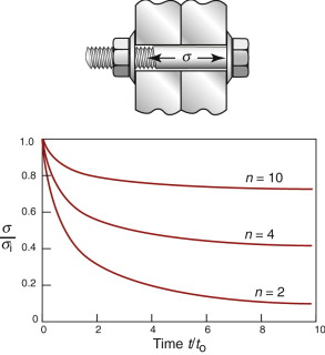

If creep strain εcr replaces part of εel the stress relaxes. At any time t
This total strain εtot is fixed because the component on which the bolt is clamped is rigid. Differentiating with respect to time, inserting equation (13.3) for ![]() gives
gives
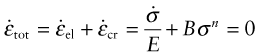
The time t for the stress to relax from σi to σ, for n > 1, is found by integrating over time:
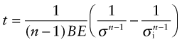
Solving for σ/σi as a function of t gives
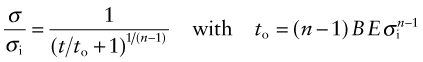
The stress σ/σi is plotted as a function of t/to in Figure 13.26, for three values of n. The relaxation is most extensive when n is small. As it rises, the drop in stress becomes less until, as n approaches infinity, meaning rate-independent plasticity, it disappears. Since transient creep is neglected, these curves overestimate the relaxation time for the first tightening of the bolt, but improve for longer times.
13.7 Summary and conclusions
All material properties depend on temperature. Some, like the density and the modulus, change relatively little and in a predictable way, making compensation easy. Transport properties, meaning thermal conductivity and conductivity for matter flow (which we call diffusion), change in more complex ways. The last of these—diffusion—has a profound effect on mechanical properties when temperatures are high. To understand and use diffusion we need the idea of thermal activation—the ability of atoms to jump from one site to another, using thermal energy as the springboard. In crystals, atoms jump from vacancy to vacancy, but in glasses, with no fixed lattice sites, the jumps occur when enough free volume comes together to make an atom-sized hole. This atom motion allows the intermixing of atoms in a concentration gradient. External stress, too, drives a flux of atoms, causing the material to change shape in a way that allows the stress to do work.
Diffusion plays a fundamental role in the processing of materials, the subject of Chapters 18 and 19. It is also diffusion that causes creep and creep fracture. Their rates increase exponentially with temperature, introducing the first challenge for design: that of predicting the rates with useful accuracy. Exponential rates require precise data—small changes in activation energy give large changes in rates—and these data are hard to measure and are sensitive to slight changes of composition. And there is more than one mechanism of creep, compounding the problem. The mechanisms compete, the one giving the fastest rate winning. If you design using data and formulae for one, but under service conditions another is dominant, you are in trouble. Deformation mechanism maps help here, identifying both the mechanism and the approximate rate of creep.
A consequence of all this is that materials selection for high-temperature design, and the design itself, is based largely on empirical data rather than on modeling of the sort used for elastic and plastic design in Chapters 5, 7 and 10. Empirical data means plots, for individual alloys, of the creep strain rate and life as functions of temperature and stress. For polymers a different approach is used. Because their melting points and glass temperatures are low, they are visco-elastic at room temperature. Then design can be based on plots of the creep modulus—the equivalent of Young’s modulus for a creeping material. The creep modulus at a given temperature and time is read off the plot and used in standard solutions for elastic problems (Chapter 5) to assess stress or deflection.
The chapter ends with examples of the use of some of these methods.
Cottrell A.H. The Mechanical Properties of Matter 1964 Wiley London, UK Library of Congress Number 64-14262. (Now 40 years old, inevitably somewhat dated, and now out of print, but still the best introduction to the mechanical properties of matter that I have ever found. Worth hunting for.)
Finnie I., Heller W.R. Creep of Engineering Materials 1959 McGraw-Hill New York, USA Library of Congress No. 58-11171. (Old and somewhat dated, but still an excellent introduction to creep in an engineering context.)
Frost H.J., Ashby M.F. Deformation Mechanism Maps 1982 Pergamon Press Oxford, UK ISBN 0-08-029337-9. (A monograph compiling deformation mechanism maps for a wide range of materials, with explanation of their construction.)
Penny R.K., Marriott D.L. Design for Creep 1971 McGraw-Hill New York, USA ISBN 07-094157-2. (A monograph bringing together the mechanics and the materials aspects of creep and creep fracture.)
Waterman N.A., Ashby M.F. The Elsevier Materials Selector 1991 Elsevier Applied Science Barking, UK ISBN 1-85166-605-2. (A three-volume compilation of data and charts for material properties, including creep and creep fracture.)
13.9 Exercises
- Exercise E13.1 The self-diffusion constants for aluminum are Do = 1.7 × 10⁻⁴ m2/s and Qd = 142 kJ/mol. What is the diffusion coefficient in aluminum at 400 °C?
- Exercise E13.2 A steel component is nickel-plated to give corrosion protection. To increase the strength of the bond between the steel and the nickel, the component is heated for four hours at 1000 °C. If the diffusion parameters for nickel in iron are Do = 1.9 × 10⁻⁴ m2/s and Qd = 284 kJ/mol, how far would you expect the nickel to diffuse into the steel in this time?
- Exercise E13.3 The diffusion coefficient at the melting point for materials is approximately constant, with the value D = 10−12 m2/s. What is the diffusion distance if a material is held for 12 hours at just below its melting temperature? This distance gives an idea of the maximum distance over which concentration gradients can be smoothed by diffusion.
- Exercise E13.4 What are the requirements of a creep-resistant material? What materials would you consider for use at 550 °C?
Exercise E13.5 Pipework with a radius of 20 mm and a wall thickness of 4 mm made of
 Cr Mo steel contains a hot fluid under pressure. The pressure is 10 MPa at a temperature of 600 °C. The table lists the creep constants for this steel. Calculate the creep rate of the pipe wall, assuming steady-state power-law creep.
Material Reference strain rate,  (1/s)
(1/s)Reference stress, σo (MPa) Rupture exponent, m Activation energy, Qc (kJ/mol)  Cr Mo steel
3.48 × 10¹⁰ 169 7.5 280 - Exercise E13.6 There is concern that the pipework described in the previous exercise might rupture in less than the design life of 1 year. If the Monkman–Grant constant for
 Cr Mo steel is 0.06, how long will it last before it ruptures?
 Exercise E13.7 If the creep rate of a component made of
 Cr Mo steel must not exceed 10−8/second at 500 °C, what is the greatest stress that it can safely carry? Use the data listed in the previous two examples to find out.
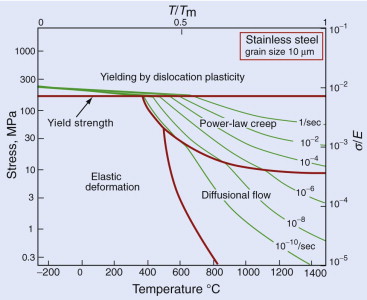
- Exercise E13.8 A stainless steel suspension cable in a furnace is subjected to a stress of 100 MPa at 700 °C. Its creep rate is found to be unacceptably high. By what mechanism is creep occurring? What action would you suggest to tackle the problem? The figure shows the deformation mechanism map for the material.
- Exercise E13.9 The wall of a pipe of the same stainless steel as that of the previous exercise carries a stress of 3 MPa at the very high temperature of 1000 °C. In this application it, too, creeps at a rate that is unacceptably high. By what mechanism is creep occurring? What action would you suggest to tackle the problem?
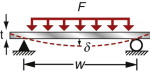
- Exercise E13.10 It is proposed to make a shelf for a hot-air drying system from acrylic sheet. The shelf is simply supported, as in the diagram, and has a width w = 500 mm, a thickness t = 8 mm and a depth b = 200 mm. It must carry a distributed load of 50 N at 60 °C with a design life of 800 hours (about a year) of continuous use. Use the creep modulus plotted in Figure 13.17 and the solution to the appropriate elastic problem (Chapter 5) to find out how much it will sag in that time.
13.10 Exploring design with CES (use Level 2 unless otherwise stated)
- Exercise E13.11 Use the Search facility in CES to find:
- Exercise E13.12 Use the CES software to make a bar chart for the glass temperatures of polymers like that for melting point in the text (Figure 13.6). What is the range of glass temperatures for polymers?
Exercise E13.13 The analysis of thermal barrier coatings formulated the design constraints. Use the selector to find the best material. Here is a summary of the constraints and the objective.
Function •Thermal barrier coating Constraints •Maximum service temperature >1300 °C •Adequate strength: σy > 400 MPa Objective •Minimise thermal conductivity λ Free variable •Choice of material - Exercise E13.14 Find materials with Tmax > 500 °C and the lowest possible thermal conductivity. Switch the database to Level 3 to get more detail. Report the three materials with the lowest thermal conductivity.
13.11 Exploring the science with CES Elements
Exercise E13.15 The claim is made in the text (equation (13.13b)) that the activation energy for self-diffusion, normalised by
 , is approximately constant for metals:
Make a bar chart of this quantity and explore the degree to which it is true.
Exercise E13.16 The claim is made in the text (equation (13.13c)) that the diffusion coefficient of metals, evaluated at their melting point, is also approximately constant:
Make a bar chart of this quantity and explore the degree to which it is true.
- Exercise E13.17 What is a ‘typical’ value for the pre-exponential, Do? Is it roughly constant for the elements? Make a chart with the activation energy for diffusion, Qd, on the x-axis and the pre-exponential Do on the y-axis to explore this.
- Exercise E13.18 The diffusive jump shown in Figure 13.9 requires that the diffusing atom breaks its bonds in its starting position in order to jump into its final one. You might, then, expect that there would be at least an approximate proportionality between the activation energy for self-diffusion Qd and the cohesive energy Hc of the material. Make a chart with Hc on the x-axis and Qd on the y-axis. Report what you find.

1 Adolph Eugen Fick (1829–1901), German physicist, physiologist and inventor of the contact lens. He formulated the law that describes the passage of gas through a membrane, but which also describes the heat-activated mixing of atoms in solids.