1.1.1 Laws of thermodynamics

As far as we understand, all matter possesses a quantity of mass and a quantity of energy. These two values are inextricably linked and we can assume that their total quantities never change – referred to as the laws of conservation of mass and conservation of energy, respectively. The reasons for this are explained in the following section. The further implications are that energy and mass are constantly moving from one place to another. Energy is formally described as the capacity of a system to do work and can occur either as potential energy (i.e. that stored in a body such as nuclear, electrical, etc.) or kinetic energy (i.e. energy of motion). The internal energy, U, of a body is the sum of potential and kinetic energies between component atoms and molecules, the total quantity of which is measured in Joules, and manifesting itself as the physical property of temperature. One can express this as a thermodynamic temperature, T in Kelvin (K) or as a Celsius temperature, θ in degrees Celsius (°C). Note that a temperature of zero on the Kelvin scale (− 273.15 °C) is called absolute zero because in theory it is the coldest possible temperature when internal kinetic energy is zero. When the temperature of matter in one region is higher than that in another region, transport of energy will attempt to occur from the hotter body to the cooler body until temperature equilibrium is restored. When energy is in transport from a higher temperature body to a lower one, it is described as heat energy. Mass is formally described in terms of its inertia (i.e. its resistance to acceleration), although it can also be measured in terms of the gravitational force it exerts on other objects, or (in practice) as the force by which it is gravitationally attracted to the Earth’s mass, i.e. its weight. Mass transfer is when transport of matter occurs from a higher concentration of mass in one region to a lower concentration in another. One can immediately appreciate how and why heat and mass transport occurs and the importance that this has within the context of this book.

A popular phrase that is used to describe the first law of thermodynamics is that ‘heat is work and work is heat’. Work, W is the fundamental physical property in thermodynamics and simply describes motion against an opposing force, i.e. 1 Joule (J) is equal to the energy needed for 1 Newton of force to push an object over a distance of 1 metre. The energy of a system can be changed either by the system doing work, doing work on the system, or by transferring energy to or from another system in the form of heat. A ‘system’ in this sense can include a control volume of a material, e.g. a collection of molecules. An ‘open system’ is one where both matter and energy are free to enter or leave. In a ‘closed system’ only energy is able to enter or leave, whilst in an ‘isolated system’ neither mass nor energy can enter or leave. In a non-isolated system, the internal energy (U), can be changed by the transport of mass, transport of heat energy (Q; unit = Watts), or by the system doing work. An adiabatic system is one where, theoretically, there is no transfer of heat. The first law of thermodynamics can now be written such that for an adiabatic system Q = 0 and so ΔU = W, whereas in a non-adiabatic system ΔU = Q + W, i.e. the conservation of energy law applies. We can expand this to include the concept of enthalpy, H, which describes the thermodynamic potential of a system, summing internal energy and the product of pressure and volume so that H = U + PV.

The second law of thermodynamics can be explained by the assertion that heat energy cannot of itself pass from one body to a hotter body. This suggests that the natural process of heat transfer is irreversible since heat cannot pass between two systems in thermal equilibrium with one another, nor can it pass from a cooler system to a hotter one. From this observation we create the concept of entropy, S which is a measure of the unavailability of energy to do work. The second law can be used to relate temperature and entropy to heat input/output, Q from a non-isolated system. This enables us to re-write the first law equation as ΔU = TΔS − W. Following on from the previous explanation of the first law of thermodynamics, we can combine this with the second law under Clausius’ Dictum, which states that the total amount of heat energy in an isolated system is constant and the entropy of the system tends to increase (over time) towards a maximum. This results in a prediction known as the heat death of the universe, assuming that it is an isolated system, where entropy would tend to maximum and no more work could be done. Finally, there is the third law of thermodynamics and the zeroth law of thermodynamics. The third law states that for a perfect crystalline solid at absolute zero (0 K) ΔS = 0, enabling absolute values for entropy to be stated with reference to this point. The zeroth law logically concludes that if two non-isolated systems are in equilibrium with a third system, then all systems are in equilibrium with each other.

Heat capacity is an important material property that can have significant effects on heat transfer. The specific heat capacity at constant pressure, c_p (W/kg K) is the energy required to raise the temperature of 1 kg of a material by 1 K. If the temperature difference across a material changes, the heat capacity (along with the thermal conductivity) will largely determine how long it takes for the temperature gradient to form within that material. This is an important concept and is recurring throughout this chapter and the rest of the book. For further detail on the laws of thermodynamics and their implications for the properties of matter, see Atkins’ Physical Chemistry (Atkins & De Paula, 2006).

1.1.2 Conservation laws

The conservation laws are an essential prerequisite for understanding how and why the transport of energy (in the form of heat) and mass actually occur and how it involves matter. These principles can be accurately described using classical physics, which is perfectly accurate for engineering-scale situations without resorting to a quantum mechanics approach and is more than enough for materials and building physics in this context. The classical physics approach to conservation in energy (heat) and mass transport is the foundation of the subject of transport phenomena and is dealt with very comprehensively by Bird et al. (2001) in their landmark textbook Transport Phenomena. This section provides an overview of the concepts as a prelude to heat and mass transport in materials. To begin, we must consider a material at the molecular level and we can use the simple example of one oxygen molecule (in air) colliding with another oxygen molecule (adapted from Bird et al., 2001).

According to the law of conservation of mass, the sum of masses entering and leaving the collision must be equal:

1.1

where and

According to the law of conservation of momentum, the sum of momenta entering and leaving the collision must be equal:

1.2

Note that r_A1 is the position vector of atom 1 in molecule A, whilst is the velocity of that atom and hence the linear momentum, The centre of mass of molecule A is at position vector r_A, and the distances of each atom from this point are R_A1 and R_A2, respectively. Note that r_A1 = r_A + R_A1 and that R_A1 = − R_A2, and that the same rule applies to velocity such that . This means that the conservation of momentum equation can be reduced to:

1.3

Finally, the law of conservation of energy states that the sum of the energies of the colliding molecules must be equal before and after the collision. Following on from the second law of thermodynamics, if one of the molecules has more energy (higher temperature) than the other before the collision, energy will transfer in the form of heat from the hotter molecule to the colder molecule. The interatomic potential energy, ϕ_A is the force of the chemical bond joining the atoms. The law of conservation of energy gives us:

1.4

The total energy within a molecule is the sum of kinetic energies of the atoms plus the interatomic potential energy and is given by:

1.5

From the term recall that , and that therefore the law of conservation of energy reduces to:

1.6

Note that the energy of the molecule (including vibration, rotation and potential energy), and the kinetic energy of the molecule are distinct. However, in collision with another molecule kinetic energy can be converted into internal energy and vice versa.

To summarise, in the following sections we are dealing with heat transfer which is the transport of energy as heat, and mass transfer which is the transport of mass. Clearly both involve all of the conservation laws and it is a useful starting point towards appreciating how and why the proceeding behaviours occur.

1.2.1 Dry state thermal conduction

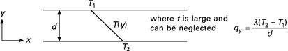
Thermal conduction is the transfer of internal energy (as heat), which occurs between neighbouring molecules of a solid, liquid or gas and between different materials in close contact with each other without the need for any bulk movement of that material. The rate of conduction heat transfer is proportional to the temperature gradient and the coefficient of proportionality is termed the thermal conductivity, λ (W/m K). As heat flows from a location of higher temperature, T (K), to one of lower temperature, heat flux q (W/m²) by conduction can be described, in one dimension, y (m), by Fourier’s Law of Thermal Conduction (see Fig. 1.1):

The temperature can vary in all three dimensions simultaneously such that the x and z axes can also be written:

1.7

The simultaneous heat fluxes in each dimension can of course be written as a single flux with temperature divergence, if the x, y, z vectors are known, to give the more general expression:

1.8

For a thermally homogeneous material of known thickness, d (mm) with surface temperatures T₁ at x = 0 and T₂ at x = d, under steady state conditions we get a steady state temperature gradient as shown in Fig. 1.2.

The thermal conductivity of a material is typically measured by a steady state method such as heat flow meter apparatus that complies with ISO 8301 Thermal Insulation – Determination of Steady State Thermal Resistance and Related Properties, or guarded hot box apparatus (BS EN ISO 8990). In the field, thermal conductivity of materials in situ can be measured by heat probe methods (Pilkington et al., 2008; Bristow, 1998), or heat flux meters (Doran, 2000). The ‘as built’ conductivity of materials is often found to be higher than the design value and this can be due to a number of factors including degradation with age, weathering, dirt and moisture accumulation, thermal bridging and construction defects. Doran found ‘as built’ U-values were on average 20% higher than design values for wall and ceiling constructions in the UK (Doran, 2000). ISO 10456 (1999) gives methodologies for the calculation of the change in thermal conductivity when influenced by variations in specimen moisture content, temperature and age based on tables of factors that are given for a number of common materials. Thermal conductivity of porous building materials can be greatly affected by their moisture content and it is important to be aware of the moisture content of the material being tested. Relationships between moisture content and thermal conductivity can be determined experimentally (ISO 10051, 1996).

For building fabric, the overall thermal transmittance, U is often termed the ‘U-value’ (W/m² K) which is simply the reciprocal of the total thermal resistance, R_T for a fabric of known thermal conductivity, λ and thickness, d. The thermal resistance or ‘R-value’ (m² K/W) of a material or layer is equal to d/λ and multiple resistances are commutative, e.g. in the case of a wall R_T = R_brick + R_{air cavity} + R_concrete + R_plasterboard. Indoor and outdoor surface resistances (R_si, R_so) can be included as discussed below. This is analogous to electrical resistance since q = ΔT/R for resistances in series. Note, in the equation above, that a thermal resistance has been attributed to the air cavity. Clearly heat transfer across a fluid-filled space in this sense would occur by natural convection although fluid conduction also occurs. The use of a single resistance term is to treat this heat transfer as a conductive term, for convenience, by expressing the equivalent resistance offered as a result of the convection coefficient in the cavity. This can be calculated in each case but standard tabulated values are normally used depending upon flow direction and whether the cavity is ventilated or unventilated. For further information and for typical values, refer to CIBSE Guide A (CIBSE, 2006). In a similar manner, the complex fluid–surface interactions that occur at the boundary when air meets the wall surface, for example, can be reduced to a single ‘equivalent resistance’ term. These values take into account the convection coefficient for any solid-fluid heat transfer, as well as short wave radiation gains by the solid, and long wave radiation gains/losses by the surface. Again, standard values for internal surface resistance (R_si) and outside surface resistance (R_so) have been produced for convenience (CIBSE, 2006).

1.2.2 Moisture-dependent thermal conduction

From the previous section it can be seen that if T₁ and T₂ are known for a material of thickness d, then λ can be calculated simply by measuring the heat flux through the material under steady state conditions. For porous materials, they absorb and store a certain amount of moisture from the air (depending upon the relative humidity) and can absorb liquid water, e.g. by rainfall or by capillarity from the ground (see Section 1.3 for more details). This has an effect on the thermal conductivity of the material that, for some materials, is very significant and for others is less so. Heat flow meter apparatus can be used to test materials in their fully dry state, when partly moist (referred to as unsaturated), or when fully saturated (Hall & Allinson, 2008a). Under steady state conditions, the thermal conductivity (λ) of the specimen is calculated using:

1.9

The values for the calibration constants of the apparatus k₁ ‒ k₆ inclusive are determined separately, and the Heat Flowmeter Output (HFM) is measured in mV. Steady state conditions are deemed to occur when the percentage variation in heat flux throughout the sample is ≤ 3%. The sample interval of the heat flow meter is given by the greater of 300 seconds or:

1.10

Prior to testing for moisture-dependent thermal conductivity, specimens (normally in the form of a thin slab) are oven dried at 105 °C to constant mass to give a moisture content of zero (Hall & Allinson, 2008a). They are then wrapped in a thin vapour-tight membrane and sealed using a small amount of adhesive around the sides (not in contact with hot/cold plates) of the specimen. They can later be unsealed and sprayed with a pre-measured quantity of distilled water before being re-sealed inside the membrane and stored under ambient conditions for 48 hours to allow the moisture to distribute within the material. This process can be repeated each time increasing the water content until the specimens are submerged in a bath of distilled water to achieve full saturation. The thermal conductivity of the membrane must be pre-determined in order to factor it out of the final calculation. The moisture content-dependant thermal conductivity of a material, λ* is defined under steady state conditions by ISO 10051 (1996):

1.11

where q_m is the measured density of heat flow rate at the hot and cold sides of the specimen (W/m²). The effect of moisture content on relative humidity was determined based on ISO 10051 (1996) Determination of Thermal Transmissivity of a Moist Material.

Since the enthalpies of water vapour and liquid water are different from one another, the total flux, g_t is equal to g_v + g_l (ISO 10051, 1996). When a temperature difference (ΔT) is applied across the specimen, the water begins to move around due to factors such as natural convection, diffusion and changes in capillary potential (see Section 1.3). In the early stages (when t is small), water close to the hot side can vaporise and migrate towards the cool side by diffusion. This has a significant effect in increasing q over that of a dry specimen since heat energy is transported sensibly by conduction through the solid and convection in the vapour, but also latently by the vapour which can condense near the cold side. As t becomes larger the accumulation of condensed water near the cold side can result in a gradient in capillary potential that induces liquid water to transport towards the warm side. Eventually the mass flux can become counterbalanced with vapour migrating from hot plate to cold plate and condensed liquid migrating from cold towards hot. Assuming that the sealed specimen contains a constant total amount of water, the counterbalancing situation is reached when:

1.12

ISO 10456 (1999) Procedures for Determining Declared and Design Thermal Values provides methodologies for the theoretical calculation of the change in thermal conductivity when influenced by, for example, variations in specimen moisture content, temperature and age. λ₂ (the corrected thermal conductivity) is calculated simply by multiplying λ₁ (the measured thermal conductivity) by the moisture conversion factor F_m, where (ISO 10456, 1999):

1.13

The mass of moisture content in the second (wetter) state, u₂, and the first (dryer) state, u₁, is expressed in mass per mass units (kg/kg), as is the moisture content conversion coefficient, f_u. A series of tables for standard values of f_u can be obtained from ISO 10456.

1.2.3 Transient thermal conduction

The heat capacity is significant when the dynamic (transient or time varying) heat transfer is considered. Two commonly used material characteristics that incorporate heat capacity are diffusivity and effusivity. Thermal diffusivity is calculated from the ratio of the thermal conductivity to the volumetric heat capacity:

1.14

Materials with a higher thermal diffusivity will reach thermal equilibrium with their surroundings more quickly. Thermal effusivity is calculated from the square root of the product of thermal conductivity and volumetric heat capacity:

1.15

It can be used to infer the magnitude of heat transfer on contact with a material. For example, if one were to touch both timber and steel at the same room temperature, the steel would feel colder as it has a higher effusivity and heat is transferred from one’s hand into the material at a higher rate.

The general form of the heat diffusion equation relies upon the conservation of energy principle (described in Section 1.1.2). It can be used as the basis to measure temperature distribution as a function of time in each of the three dimensions, T(x, y, z), and can be written as follows (Incropera et al., 2007):

1.16

Note that is a heat energy source term associated with the rate of heat generation from the material measured as Watts per unit volume of the material in question (W/m³). In a case of known dimensions, the effective length, L equals the distance between maximum and minimum points on a single temperature gradient. The quantity hL/λ is a dimensionless parameter called the Biot number (Bi) that is used in transient conduction problems involving convection exchanges. It is effectively the measure of a temperature drop in the solid relative to the temperature difference between the surface of that solid and a fluid (liquid, gas or a gas/vapour mixture such as air) (Incropera et al., 2007).

1.17

Figure 1.3 shows the effect of Biot number on the steady state temperature distribution established in a wall with surface convection at the wall–air boundary. The so-called lumped capacitance method assumes that T is uniform at any instant, even if decreasing as a function of time. This would suggest λ = ∞, or we can simply assume that temperature gradient exists but is negligible and can be ignored. When Bi < < 1 the resistance to thermal conduction within the solid is much lower than the resistance to convection across the solid–fluid boundary layer. Therefore, the assumption of a negligible thermal gradient within the solid can be valid.

The Biot number is also very useful for considering the evolution of thermal gradients inside a solid material (e.g. a wall) when the environmental conditions are changed. The example in Fig. 1.4 shows three walls and with very contrasting Biot numbers. Note that in a symmetrical case such as this, the wall thickness is taken as 2 L since the effective length is that between the peak temperature (wall centre) and the lowest point. The walls are equilibrated at initial temperature T_i, and the temperature of the surrounding air is suddenly raised to T_∞ < T_i. Note that, once more, when Bi < < 1 the thermal gradient in the solid is negligible and so in this one-dimensional case T(x, t) ≈ T(t). In contrast, when Bi > > 1 the majority of temperature difference evolves within the solid as opposed to near the solid–fluid boundary.

With reference to the thermal diffusivity, and in addition to the Biot number, the second key dimensionless term that is essential for transient conduction is the Fourier number, Fo where:

1.18

and

1.19

From this we can calculate the temperature change of the solid over a period of time or the solid temperature at a known time, t using:

1.20

In cases where the simple lumped capacitance method is invalid (e.g. where Bi > > 1), temperature gradients can no longer be assumed to be negligible and so more sophisticated numerical methods must be used. A full review of these are beyond the scope of this chapter. Further details can be obtained by referring to Incropera et al. (2007). Some specific models and techniques are discussed in further detail later in this section.

In all of the approaches to thermal conduction in building fabrics that have been discussed so far, the heat transfer has largely been assumed to be in one dimension. This is perfectly acceptable where energy efficiency and fabric heat loss/gain are the primary concerns. In situations where distribution of heat by conduction needs to be understood (e.g. due to thermal bridging around a column or a joint), then a two-dimensional or even three-dimensional approach may be required. One of the most common approaches is to use the Control Volume Method (CVM) which involves discretising the fabric in the form of a mesh, where thermal conduction between nodal points is considered. The finer the mesh, the closer the numerical result becomes to the true value; hence the complexity and scale of the mesh gives more accurate results at the expense of processing time. Many commercial software packages use an approach such as this, including FLUENT by ANSYS.

1.2.4 Thermal convection

Convection occurs when there is conduction of heat into the molecules of a fluid and the bulk motion of that fluid that carries those molecules away from the heat source. Typically it is used to describe the heat exchange at a surface due to the movement of air across that surface. The air movement may be the result of natural convection due to the buoyancy of warmed (less dense) air immediately above a flat roof for example, or through forced convection caused by wind or vehicle motion and may be a combination of the two. It can be described in a form similar to conduction but introducing a convection coefficient, h_c (W/m² K):

1.21

The value of the convection coefficient will depend on geometry (shape and orientation of surface), material properties (surface roughness), fluid properties (viscosity), fluid free stream velocity (speed and direction) and the temperature of the bulk fluid and the surface. These will determine whether the flow over the surface is buoyancy driven or forced, laminar or turbulent or, in fact, a combination of these. The complexity of the fluid dynamics has lead to the use of simplified empirical calculations. A couple of examples are given below and more can be found in recommended papers such as Cole and Sturrock (1977), McClellan and Pedersen (1997) and Liesen and Pedersen (1997). The CIBSE Guide C (2007) proposes a simple method of calculating the convection coefficient for external surfaces at any wind speed, c_s (m/s) based on empirical wind tunnel experiments:

1.22

Standard BS EN 15026 (2007) gives a similar correlation (h_c = 4 + 4 c_s) and includes a note that c_s has to be measured near the building’s surface, which is often not rigorously pursued in practice. It is important to point out at this stage that determining a correlation between the unobstructed wind speed at 10 m height above ground (unobstructed wind) and the surface resistance is very useful but that if this is not possible then constant values that have been validated for building applications should be used instead. An empirical method for calculating surface wind speed from the unobstructed wind speed is given in the ASHRAE Handbook (ASHRAE, 2005).

The ASHRAE detailed algorithm (Energy Plus Engineering Reference Online, 2009) considers that the exterior convection coefficient comprises components due to natural convection, h_n, and forced convection, h_f, such that h_c = h_n + h_f. The natural convection coefficient is described by Eq.1. 23 for upward heat flow and Eq. 1.24 for downward heat flow:

1.23

1.24

Note that ϕ is the angle of the surface from the horizontal. The forced convection coefficient is calculated from surface geometry, surface roughness and wind speed:

1.25

where W_f relates to surface orientation (1 for windward surfaces), R_f is a roughness index (ranging from 2.17 for very rough to 1.00 for very smooth), P is the perimeter of the exposed surface (m), v_z the local wind speed (m/s) and A the surface area of the fabric (m²). The choice of calculation method can make significant differences to the convection coefficient and ultimately the heat transfer and therefore care must be taken to validate models wherever possible. It should, however, be remembered that knowledge of the air speed at the surface may be equally important to the accuracy of any simulation and this can be difficult to determine, especially for the microclimate around vehicles and structures.

Convection heat transfer also occurs inside porous materials, and it is the reduction in this term that gives insulating materials their low heat transfer properties. Solid insulation materials normally have a low density and contain a large proportion of pores (or voids) that are inter-connected such that they offer a very high level of resistance to any fluids attempting to pass through them, i.e. tortuosity (see Section 1.3 for further details). The purpose of so-called ‘insulating materials’ is to offer a very high level of thermal resistance (R, m² K/W) and to be as thin as possible, i.e. λ must be very low to ensure d does not have to increase. As with all materials, we know that the total thermal conductivity of an insulation material, λ_total is quantified with respect to the heat flux under steady state conditions at a known mean temperature. Consequently, the primary modes of heat transfer through insulating materials can be considered to have a cumulative effect in determining λ_total. The heat transfer modes in a typical porous insulation material can be described as:

Note that convective and radiative terms have been lumped as effective conductions, where

1.26

Clearly, in the case of building physics, the fluid can be air, air–water mixture or water, in which case λ_fluid can vary significantly and heat energy can also pass in latent form due to vaporisation/condensation of water as discussed in Section 1.2.2. This can have serious implications for the performance of insulation materials and highlights the obvious need for them to remain dry if they are to be effective. In conventional insulation materials with pore diameters greater than ~ 1 mm, the convective heat transfer component can represent a significant proportion of λ_total at standard temperature and pressure (STP). As pore diameters become smaller and the inter-connected paths between them become more tortuous, the movement of fluid becomes restricted and so convection becomes less dominant and the thermal conductivity of the quiescent fluid phase becomes the limiting factor. If we assume that the pores are filled with air, then quiescent air has a thermal conductivity of approximately 0.026 W/m K. If the pore diameters are sufficiently small then we can assume λ_conv = 0.

In order for λ_total < 0.026 (W/m K) to occur, λ_fluid must be significantly reduced. The molecules in the fluid transfer kinetic energy to one another in the form of heat when they collide. The mean molecular free path is the average distance one of the molecules must travel before it collides with another of the same type. Therefore if this distance is reduced then λ_fluid must decrease because more molecular collisions need to happen in order to transfer the same quantity of heat energy across a distance d than before, which of course is statistically much less likely. The mean molecular free path in porous materials is reduced when the pore diameter becomes sufficiently small that molecule–pore wall collisions are statistically more likely than molecule–molecule collisions (Bird et al., 2001).

The ratio of the mean molecular free path to a characteristic length (e.g. the mean pore radius in a porous material) is referred to as the Knudsen number which uses the symbol Kn. Note that in very permeable materials when Kn > > 1 it may be necessary to use the Monte Carlo method (or similar approach) to estimate the molecular trajectories inside the pore and hence predict the number of collisions. The net result is that when Kn ≥ 1, λ_fluid can be written as:

1.27

where is the thermal conductivity of quiescent air, and α is a constant specific to the gas in the pores that is usually considered to be about 2 for air. Some solid porous insulation materials have extremely small pore diameters resulting in Knudsen numbers of about 1 to 2. This would give a λ_fluid term of between about 0.0052 and 0.0087 W/m K. It is important to understand these phenomena because lately there has been increased attention towards ‘nano insulation materials’, such as aerogels (see Chapter 13), offering a high performance alternative to other thin insulation technologies such as vacuum insulation panels (VIPs, see Chapter 8). This means that because of the low λ_fluid in reality, a λ_total value of 0.016 W/m K or less can easily be achieved.

1.2.5 Thermal radiation

Thermal radiation is electromagnetic radiation that is emitted by a body as a result of its temperature. All objects with a temperature above absolute zero emit thermal radiation in a spectrum of wavelengths. The amount of radiation emitted by a black body at any one wavelength is described by the spectral black body emissive power distribution or Planck’s Law, which may be written as:

1.28

Plotting the spectral emissive power for a black body against wavelength for a number of temperatures produces a series of curves, known as Planck’s curves, as shown in Fig. 1.5.

The total emissive power can be found by integrating Planck’s law from λ = 0 to λ = ∞ (which gives us the area under the curve for a particular temperature) and is known as the Stefan–Boltzmann law:

1.29

where σ is the Stefan–Boltzmann constant (σ = 5.669 × 10^− 8 W/m² K⁴). The ratio of the emissive power, E, of a surface to the emissive power of a blackbody, E_b, at the same temperature is known as the emissivity, ε (i.e. ε = E/E_b), therefore:

1.30

A black body is defined as a body that absorbs all incident radiation at any given temperature and wavelength. Real surfaces, however, absorb and reflect thermal radiation and may also transmit thermal radiation, as shown in Fig. 1.6, and this behaviour can vary with temperature and wavelength.

Kirchoff’s law tells us that the amount of radiative energy emitted by a surface must equal the amount of radiative energy absorbed by that surface. The material properties of interest are therefore the absorbtivity (α) or emissivity (ε), reflectivity (ρ) and transmissivity (τ), which describe the fractions of the incident radiation that are absorbed, reflected and transmitted such that α + ρ + τ = 1 and ε = α.

The net radiant heat transfer between two surfaces is dependent on their temperatures, sizes and view factors. Radiation view factors describe the fraction of the surface area of the hemispherical view from a surface that comprises the other surface. Techniques for determining view factors include mathematical, reference tables, ray tracing and fish eye lens photography and other methods that can be applied to urban areas (Grimmond et al., 2001). An example of their use would be for the long wave radiative heat exchange between a surface and the external environment. This could be divided into that between the surface and the ground, F_gnd, the surface and background objects, F_bg, and the surface and the sky, F_sky. Assuming temperature could be assigned to each of these: T_gnd, T_bg and T_sky, according to Mcclellan and Pedersen (1997) the radiative heat exchange at the surface can be simplified to:

1.31

where F_gnd + F_bg + F_sky = 1. The determination of the ground, background and sky temperatures must also be considered. For inside surfaces such as the walls, floor and ceiling of a room, other methods have been developed such as the one described by Liesen and Pedersen (1997).

Radiation that originates from the sun, which has a black body temperature of around 6000 K, has a much shorter wavelength than that from objects at typical terrestrial temperature and for this reason is termed short wave (SW) radiation. This is a useful distinction as a material’s wavelength dependent behaviour to thermal radiation can be split into LW and SW for convenience. A commonly used example is snow, which has a very low emissivity in the short wave (highly reflective) and a very high emissivity in the long wave (highly absorbent). The gas molecules and solid particulates that make up the earth’s atmosphere absorb, reflect and scatter solar radiation; the intensity at the surface is therefore dependent on the sun’s relative position and the atmospheric conditions. Cloud cover is an obvious example of this dependence. The solar radiation that is incident on a surface can be divided into that direct from the sun, diffuse radiation from the sky and reflected radiation from the ground and other surfaces. When the surface is transparent, such as glass, a portion of this radiation will be transmitted into the room, a portion reflected away from the surface and a portion absorbed by the glass. Different methods for calculating these effects have been developed (see, for example, CIBSE, 2006 and McClellan and Pedersen, 1997).

1.2.6 Steady state environmental parameters

The ratio of temperature change across a boundary is proportional to the ratio of thermal resistances such that (McMullan, 1992):

1.32

where ΔT = temperature difference across a layer, T_T = total temperature difference across the element, R = resistance of that layer, and R_T = total resistance of the element. The formula can simply be rearranged to give the temperature difference (ΔT) across each boundary layer within a multilayer fabric, e.g. a wall. This technique is referred to as the Glaser Method and is illustrated in Fig. 1.7.

Surface resistances are included to make surface temperatures more realistic; these are usually taken as tabulated values from the CIBSE Guide A (2006) or similar. The choice of values depends upon level of exposure and air velocity near the surface, e.g. typical R_si = 0.123 m² K/W. A similar approach is taken for air pockets, for example in a cavity wall where standard values are assumed for ventilated or unventilated cavities. The main weakness of this model is that the two temperature set points (T₁ and T₂) are taken from indoor/outdoor air temperatures which ignores additional gains or losses through the fabric as a result of radiation or convection. This is important because the temperature profile will be less accurate and surface temperatures can be very inaccurate, e.g. on a hot sunny day surface temperature can exceed air temperature due to solar gain but a standard Glaser model would show it as being lower.

These problems can be overcome by using a more complex Glaser method which uses nodal points as opposed to fixed air temperatures. These nodal points are hypothetical ‘equivalent’ temperatures that lump together a more complete variety of heat energy inputs. Instead of an outdoor air temperature point, a sol-air temperature node is used; a hypothetical temperature that includes the outside air temperature, SW radiation gains (from the sun), LW radiation gains from surrounding objects, and convective exchanges. The indoor air temperature is replaced by two nodal points: environmental temperature node and air temperature node. The environmental node includes convection from the room air, and radiation both from surrounding objects and direct sources, e.g. heaters/plant. Heat transfer occurs between the environmental node and the indoor air which is limited by the air convection transfer coefficient. Heat transfer from the sol-air node occurs directly to the indoor air node only in the case of infiltration (leakage), and to the environmental node in the form of conduction or conduction equivalents, i.e. it is regulated by fabric resistance R_T. The nodal network diagram in Fig. 1.8 illustrates this model.

1.2.7 Transient environmental parameters

The nodal diagram shown in Fig. 1.8 is used under steady state environmental conditions, where nodal temperatures are fixed values, e.g. using only the mean value for a day, month or season. However, it can also be extended for use with dynamic environmental conditions where the sol–air and environmental node temperatures fluctuate between maxima and minima about a mean. This principle is employed in the cyclic admittance method (see CIBSE Guide A, 2006) where the periodic fluctuation about mean values is taken to be a sinusoidal frequency pulse, normally over a duration of 24 hours. This approach has the disadvantage that the resistances (and hence the associated material properties) are assumed to be constant, which if rigorously pursued is invalid except under steady state conditions since λ is temperature dependent. However, the accuracy is normally perfectly acceptable across the temperatures ranges used in building physics. Obviously the sinusoidal temperature fluctuations are also an assumption because 24 hour cycle temperature changes do not follow this precise pattern. However, this assumption does offer the advantage of being able to compare the behaviour of one cross-sectional fabric with another under identical time-dependent environmental conditions. In order to adapt the nodal diagram for dynamic environmental conditions the terminology is changed slightly, as shown in Fig. 1.9.

Note that the Celsius temperatures and nodal heat inputs/outputs are shown with a tilde symbol to denote fluctuation which occurs simply as a function of time. The other significant change is the replacement of steady state transmittance, U, with thermal admittance, Y, for fabric conduction, where U is the rate of heat transfer across a fabric, and Y is the rate of transfer to the fabric, with identical units (W/m² K). Unlike U, which is simply the reciprocal of R_T, Y is calculated using a set of matrices which employ density, heat capacity, thickness and thermal conductivity (see CIBSE Guide A, 2006). As a result, heat transfer from the environmental node to the fabric (and subsequent storage of heat energy) can be approximated using the admittance method which is useful for determining any reductions in peak cooling loads inside a building. High thermal admittance is one of the two most important features of fabrics that are referred to as having ‘thermal mass’. This is also an important concept when considering passive cooling as a result of fabric energy storage, and is discussed in more detail in Chapter 4.

The second important feature of thermal mass fabrics is that of thermal decrement factor, f. This is used to represent the reduction in temperature gradient formation (as a function of time) across a fabric as a result of heat storage within that fabric, and hence the rate of heat transfer is attenuated by the factor f. This forms an additional component to calculating peak cooling load. It can also be used in conjunction with the nodal diagram for a sol–air temperature fluctuating as a function of time, t, to approximate the response of the environmental node temperature which of course now fluctuates as a function of f. In this situation, decrement has an associated time lag, ϕ (hours), which causes the maxima and minima to move out of phase with the sol–air node temperature as shown in Fig. 1.10.

The consequences of this behaviour are that low thermal mass walls tend to exhibit less attenuation of environmental temperatures (dashed lines) in response to sol–air fluctuations (solid lines) and with a shorter decrement time lag than do high thermal mass walls. This translates to reduced potential for heat transfer from the environmental node to the indoor air node since the temperature gradients between the two will be lower. Since thermostatic controls for HVAC systems typically use indoor air temperatures, high decrement fabrics can (in theory) be used to reduce the heating cooling loads considerably. One final point is that since decrement applies to heat transfer across the fabric, it is used to attenuate U as opposed to Y for heat loss/gain to the environmental node. This is very important for building fabric design because it is possible to optimise material type, thickness and positioning in relation to heat gain/loss (U), passive cooling (Y), and suppression of temperature fluctuation (f, ϕ). Examples are given in Fig. 1.11 using different configurations of a 300 mm dense concrete wall with 100 mm of polystyrene insulation.

The U value is essentially unaffected by positioning of the insulation, but admittance and decrement both are. Internal insulation gives very low admittance, opposite for external insulation. It is possible to have too much mass in one place; if it is too thick it is harder for heat energy to pass deeply enough from the environmental node in sufficient time and it starts to ‘leak’ towards the sol–air node. Optimum thicknesses of the high thermal mass material (in this case concrete) exist; they must be positioned on the inside in contact with environment and air. The exact thickness varies with material properties but for conventional mass materials (e.g. dense brick, concrete, compressed earth) this value is between 100 and 200 mm. Commercial software packages that use this approach for modelling heat transfer with transient environmental conditions include Ecotect and HEVACOMP, and it is the approved method for CIBSE.

An alternative approach to the admittance method is to use a ‘heat balance method’ approach. This looks at the cross-sectional fabric as above by considering the resistive/capacitive thermal properties, but more realistically simulates heat energy fluxes to and from the fabric. For further details of this method refer to the ASHRAE Fundamentals set of handbooks. For 2D and 3D problems the usual approach is to use a CVM for numerical modelling or a commercial package such as FLUENT. The various approaches and techniques to modelling heat transfer are beyond the scope of this chapter. The admittance and heat balance methods are discussed in more detail in Chapter 4 with particular regard to their application for thermal storage and cooling loads.

1.3.1 Psychrometrics

Psychrometrics (as distinct from psychometrics) is the study of the thermodynamic properties of air–vapour mixtures, typically focusing on the interrelation among temperature, partial pressures and enthalpy. Under normal atmospheric conditions the air in our atmosphere (mainly N₂, O₂, CO₂ plus others) contains varying amounts of water molecules in vapour state. The moisture content of air is defined as the mass of water vapour molecules per unit mass of air molecules within a finite volume and is expressed in kg/kg. The pressure of a gas (air) or vapour (e.g. water) is the result of the mean kinetic energy associated with the Brownian motion of its molecules. We know from Dalton’s Law that when two gases are mixed, in this case air and water vapour, that the total pressure of the mixture is equal to the sum of the two pressures which are now called partial pressures. We also know from this law that partial pressures are commutative such that if the partial vapour pressure (per unit volume) increases, the air pressure stays the same and the total pressure increases by Δp_v. The relative humidity, φ, of the air–vapour mixture is defined as the partial vapour pressure as a proportion of the saturation vapour pressure within a finite volume at known temperature. It can be given either as the decimal value of the fraction p_v/ p_vsat or as a percentage. Note that the dew point temperature is the point at which water vapour in a known volume of air will condense, since it occurs at the point where φ → 1 (or 100% RH). If a bulb thermometer is placed in the air–vapour mixture, the temperature recorded is a consequence of the internal energies of the gas and vapour, and is referred to as the dry bulb temperature. If the thermometer bulb is then surrounded by a wick saturated in liquid water, evaporation from the wick occurs, the rate of which is controlled by the temperature and moisture content of the surrounding air. Evaporative cooling of the surface results in a reduction of the measured temperature (called the wet bulb temperature), and the depression between this and dry bulb directly corresponds to the relative humidity of the air. On this basis, a psychrometric chart (see Chapter 4 for further details) can be plotted linking dry bulb and wet bulb temperatures to corresponding relative humidities, which in turn have corresponding partial vapour pressures (and therefore moisture contents) and dew point temperatures. Note that the enthalpy of the air corresponds to the sum of the internal energies of the gas molecules and water vapour molecules.

1.3.2 Porous materials

Porous materials contain voids (or pores), either in isolation or interconnected to form complex networks of channels, which are filled with fluid under normal atmospheric conditions, e.g. air, liquid water, or air and water vapour. Depending upon the permeability of the material, fluids are able to enter or leave the voids and to move along within continuous voids. Therefore, all permeable materials are porous but the degree to which porous materials are permeable varies considerably. It can even tend towards zero for materials with isolated or closed voids. The permeability of a porous material can be quantified and expressed as a coefficient to describe the restrictions imposed on fluid flow. These restrictions can be attributed to a wide range of parameters such as the total volume of void space (i.e. bulk porosity, n), the void size distribution, the extent of interconnectivity between voids, as well as minor factors such as the roughness of void interior surfaces. One other important factor is tortuosity, because we may have implicitly assumed up until this point that the interconnected voids are all straight with no corners or bends. When fluid is travelling from one point to another inside a continuous void the resistance to flow increases if the path becomes more ‘tortuous’ or challenging. This is due to the cumulative effect of the required number of changes in flow direction, the extent to which direction must be changed, variations in void diameter, and other possible examples. The permeability of porous materials is dealt with in more detail in Section 1.3.5.

If the specimen of a porous material has a total volume, V_T, which consists of solid state matter, V_s, and fluid-filled void, V_v, then V_T ≡ V_s + V_v (see Fig. 1.12). Under atmospheric conditions, when the material is dry the voids are filled with air (V_v = V_a) and when saturated the voids are filled with water (V_v = V_w). An interesting observation is that, when water enters a dry or partly dry (known as ‘unsaturated’) porous material, it must displace an equal volume of air from the moment it crosses the boundaries defined by V_T; assuming the air to be incompressible. What can actually happen is that air is not always able to be displaced, which can prevent saturation occurring, and can even become trapped by advancing water at the ends of sealed voids with no escape. Its only option is to slowly dissolve in the water but this can take several months to occur. For these reasons full saturation rarely occurs except where the air in a porous material is first fully evacuated by placing in a vacuum chamber, and then introducing water to the sealed chamber and immersing the specimen; a process called vacuum saturation. Of course, one or more isolated pores can remain inaccessible to water even under these conditions since they are not connected to the rest of the void network. In this sense, the only true way to assess bulk porosity is to determine the specific gravity of the solid material, and gravimetrically determine the specimen’s mass as a fraction of maximum theoretical mass, where n = 0. Therefore, determining the porosity by gravimetrically measuring the maximum mass, of fluid that the voids can hold gives us the apparent density of the material or, conversely, the apparent percentage water absorption.

When water enters the finite volume that we have described as V_T (by entering the voids), we describe the process as absorption. Absorbed water molecules may also be ‘adsorbed’ to the internal surfaces of voids by van der Waals forces (since water molecules are polar). Absorbed water can be classified into one of three domains known as hygroscopic water, capillary water and gravitational water (Hall & Allinson, 2009a). The classification of the water is dependent upon (i) its phase (vapour or liquid) when it enters V_T, and (ii) the extent to which it is electrostatically attracted to the inside surfaces of the void. Hygroscopic water is absorbed as a vapour phase, capillary water is absorbed as a liquid phase, and gravitational water is liquid that is absorbed when the capillary potential in the pore network is zero (i.e. super saturation). This latter point can be better understood following an appreciation of the phenomenon known as capillarity, as described in detail in Section 1.3.4. Suffice to say that the threshold between capillary and gravitational water is the point where electrostatic attraction between the water molecules and the void surfaces is insufficient to oppose the force due to gravity.

It is helpful to describe the water content of a porous material in terms of relative water content, θ. This is in fact a dimensionless value for the water content and can be calculated using (Hall, 1977):

1.33

where 0 ≤ θ ≤ 1. Note that w = gravimetrically determined water content (kg/m³), and that w_a = minimum moisture content and w_b = maximum moisture content. In the following sections we will see how several critical values for θ occur, and that their numerical values are (i) characteristic of particular materials, and (ii) correspond to the three domains of absorbed water described above.

1.3.3 Kelvin’s equation and sorption isotherms

Since water molecules are dipolar they can attract and bond to one another through a type of van der Waals force known as hydrogen bonding. The internal molecular attractive forces in water may be termed cohesion, whilst the forces of attraction that exist between water molecules and those of dissimilar materials (e.g. the negative charged surface of a void) may be termed adhesion. If the adhesion forces between water and a dissimilar solid (e.g. glass) are greater than the intermolecular forces within the water, then the surface of the glass becomes ‘wet’ (Bowles, 1984). The formation of droplets occurs because the internal intermolecular forces of a finite amount of water are in equilibrium with the atmospheric pressure of the surrounding air (see Fig. 1.13). Since the thickness of the surface tension ‘skin’ is molecular, it follows that the unit for surface tension is force/length (Bowles, 1984). The internal/external pressure difference, known as p (where p = p_i − p_o), inside the curved surface of the droplet is directly proportional to the surface tension γ, and therefore inversely proportional to the radius of curvature r (see Fig. 1.16). This is shown by the equation below where:

1.34

Although the classification of absorbed water (determined by its phase upon entry) cannot change, its phase once inside V_T can change, for example the condensing of hygroscopic water from vapour to liquid phase (Hall & Allinson, 2009a). This phase changing can occur depending upon factors such as geometry of the voids and electrostatic surface charge within the voids. The reason for this is the simple fact that the saturation vapour pressure above a curved surface of water is different from that of a completely flat surface. The saturation vapour pressure above a flat surface of liquid water, p_sat* (when r = ∞), is dependent upon the pressure applied to that liquid by the surrounding air. For a given air pressure, the saturation vapour pressure of the water becomes (Atkins & De Paula, 2006). When the surface of the water is curved to a known radius, r, a pressure change (negative for water) occurs where ΔP = −2γ/r (see above for droplet). Note that ΔP is referred to as the capillary potential, Ψ, which is used to quantify the motivation for capillarity and is often termed ‘suction’ because it is a negative pressure differential measured in Pascals. We can see that the saturation vapour pressure of water held inside a pore of radius r (and having a contact angle α) is less than that of a flat surface, i.e. p_sat < p_sat*. This of course leads to Kelvin’s equation, where V_m = molar volume of water (~ 18 ml at STP), and R₀ = the gas constant (Atkins & De Paula, 2006). In the case of hygroscopic moisture (vapour phase, of known partial pressure) that has been absorbed by a void, Kelvin’s equation can simply be rearranged to find the ‘critical radius’ of that void (r_crit), assuming p_v = p_sat. At this point moisture vapour condenses inside the pore to restore thermodynamic equilibrium. Obviously, where radii vary within complex pore structures, it follows that vapour condenses to fill the pore with liquid when r < r_crit, and vice versa. This can lead to an interesting phenomenon known as the ‘ink bottle effect’, where a larger void has only narrow entry points. If r < r_crit at the entry points, but r > r_crit within the large void itself, then vapour can condense in the entry points effectively blocking the void from absorption or desorption. Kelvin’s equation can also be re-written so that if void radius is known, then the relative humidity, φ, of air (where φ = p_v/p_sat) at which condensation will occur is given by:

1.35

where R_vap is the gas constant for water vapour (J/kg K) and ρ_w the density of liquid water (kg/m³). It follows that in a porous material there are a wide range of voids and void sizes. As relative humidity increases the hygroscopic water increases, and so does the potential for some of this to condense to liquid inside the material because r_crit increases. Therefore at constant temperature, there is an equilibrium moisture content (EMC) for every value of φ between 0 and 1 (some of which will condense if r < r_crit) that is characteristic of each porous material. Furthermore, some of the absorbed water molecules can be adsorbed by the surfaces of the void which raises their enthalpy of vaporisation correspondingly. This results in hysteresis between the EMC when Δφ is positive (progressive wetting), and when Δφ is negative (progressive drying). By plotting moisture content against φ, a pair of sorption isotherms (or ‘moisture storage functions’) can be plotted for a particular material: a wetting isotherm and a drying isotherm (see Fig. 1.14). The gradient of an isotherm (below θ₈₀, where capillary condensation makes the isotherm slope increase rapidly) gives us a single value known as the sorption capacity, ξ. Once a material’s sorption isotherms have been characterised in this way, the EMC can be interpolated for any value of φ. Note that if φ periodically fluctuates as a function of time, the EMC corresponds to the values on the wetting isotherm for the periods of time when Δφ is positive, and then jumps across to the drying isotherm for the periods of time when Δφ is negative. It is important to distinguish that the sorption isotherm enables us to predict how much time is needed for the moisture content to reach EMC once Δφ has occurred. The response time of the material to Δφ is measured separately using the moisture buffer value (MBV) test (DTU, 2005). Some materials have relatively high moisture storage functions (i.e. steep isotherm gradients) but low MBVs, which could be interpreted as having a larger capacity to store moisture as a function of φ, but a slower response time to changes in φ as a function of time. Other materials exhibit the opposite sort of behaviour, i.e. quick response times but lower storage capacity. The behaviour of materials in this respect is discussed in more detail in Chapter 14.

The sorption isotherm in Fig. 1.14 also shows that at very low relative humidity, single layer adsorption followed by multi-layer adsorption of water vapour molecules occurs within the pore structure of the material. Metastable groups of adsorbed water vapour molecules can spontaneously nucleate into a liquid water meniscus that is in equilibrium with the relative humidity for a given pore radius (Hall & Allinson, 2009a). It is unclear how valid the assumptions of Kelvin’s equation become when the theoretical values for r_crit (which are constants at known T) reach this scale. It is logical to assume that the validity applies to the portion of a sorption isotherm where capillary condensation will occur in pore radii sufficient to permit thicknesses greater than multi-molecular layers (i.e. droplets) which typically occur at φ ≈ 0.5. Despite this, the occurrence of significant liquid water flow (induced by dΨ/ dx) is typically not considered until φ > 0.8 (Künzel, 1995). The reference moisture content for this value is referred to as θ₈₀ as shown in Fig. 1.14. Another point of interest on the sorption isotherm is the transition from hygroscopic domain to the capillary domain, which occurs at the hypothetical point when φ → 1 (Hall & Allinson, 2009a). This corresponds to the value known as the residual moisture content, θ_r, which has to be interpolated as opposed to measured experimentally. For numerical modelling, the maximum hygroscopic moisture content that can be readily determined experimentally is normally taken to be 95 or 98% (Künzel, 1995; Valen, 1998). When θ is in the capillary domain, water transport is dominated by capillary potential, Ψ, or ‘suction’ (Pa) and the microstructure is referred to as ‘unsaturated’.

1.3.4 Capillarity

Capillarity (or capillary suction) is the natural phenomenon that many of us have experienced at an early age by placing one end of a narrow tube in a tray of water and observing the rise of water inside the tube. We may also notice, by using a range of different width tubes, that as the radius decreases the height to which the water rises will increase. Referring to the portion of the sorption isotherm (see Fig. 1.14) above the residual water content, θ_r, we can see the so-called capillary domain. During wetting, absorption will continue until the relative water content is at capillary saturation, θ_c, at which point the total water pressure P_w = P_a − (2γ/r + ρ_wgh), for the supported mass of water inside the pore structure (where g is the gravitational constant 9.81 m/s²) (Atkins & De Paula, 2006). We already know that saturation vapour pressure above a curved water surface is different from that above a flat surface by the Kelvin equation. Water rises inside the capillary simply to offset the pressure differential between the water and the surrounding air (which includes air + water vapour). The maximum theoretical height that the column of water can achieve in a fully wet capillary is then given by:

1.36

As previously mentioned, gravitational water is liquid that is absorbed when the capillary potential in the voids is close to zero. We now know that this is additional water absorbed when the relative moisture content is > θ_c. When θ > > θ_c we refer to this as the gravitational domain although it is often known as ‘super saturation’, because the water theoretically cannot enter by capillarity. It is perhaps obvious that, if θ_c < < θ_s then additional water can be absorbed without capillarity (e.g. due to a pressure differential, gravity, etc.), some of which can be supported by remaining net surface charge in the void internal surfaces. Thus, on the drying curve the maximum capillary water content is determined by the air entry value which is designated θ_AEV. At the threshold for ‘super saturation’ (> θ_AEV) the force due to gravity on the additional mass of the non-capillary (or gravitational) water is greater than the attraction of the remaining net surface charge inside the pore structure.

Vos and Tammes (1968) performed various experiments on the capillary movement of water and concluded that, amongst other things, water moving through a porous material by capillarity could travel twice as far in a horizontal direction as in an upward direction. This is because, in the latter case, the direction of flow is perpendicular to the force of gravity and so its effect in opposing the flow is at a minimum. If a temperature gradient exists along a capillary vessel, the flow of water within that capillary will occur in the direction of the lower temperature (Vos & Tammes, 1968). This is because the electrostatic potential of the void internal surfaces is a monotonously decreasing function of temperature. This occurs because of the principles surrounding the conservation of energy in a system. If a pocket of water is held in a cylindrical void of uniform diameter, and one end of the void is heated, the water moves towards the colder end. In addition, water that is held within a void of uniform temperature, but that has a tapering diameter, will move towards the narrower end of the capillary through inducement by the higher capillary potential. The actual electrostatic charge of the void’s internal surfaces is assumed to be the same, and so when the void radius decreases towards the tapered end, the term 2γ/r becomes larger which increases Ψ. Consequently, if two porous materials are in contact with one another, water transport will occur from the larger diameter voids into the smaller diameter voids. This process occurs until the net gradient of pressure differentials has equilibrated (Vos & Tammes, 1969).

Capillary conduction describes the flow of liquid water through the pore network. If the water content is sufficiently high (i.e. capillary saturation), then Ψ = 0 and the rate of flow of the water is governed by (i) fluid pressure differential and (ii) the resistance to flow offered by the material’s pore network, e.g. due to tortuosity. This saturated flow is governed by Darcy’s law and is explained in more detail in Section 1.3.5. When the water content is between θ_r and θ_AEV, the material is ‘unsaturated’. The gradient of capillary potential, Ψ (or ‘suction’) provides the motivation force for liquid transport in unsaturated porous materials. The liquid conductivity, K (s/m) is therefore dependent on capillary potential, and so the liquid water flux can be written as:

1.37

We can see from Fig. 1.15 that Ψ can become extremely high in the hygroscopic domain and devices for measuring suction pressures (potentiometers) are typically designed for the capillary domain, making them incapable of measuring suction pressures of this magnitude. However, we know that Ψ = ΔP = 2γ/r and so we now have the relationship:

1.38

In this way, capillary potential can be approximated from the EMC corresponding to a given relative humidity, φ. In an applied sense, when capillary domain water is absorbed into porous building materials a number of complexities can arise at various stages of the process. Hall (1977) used the classic example of a dry brick placed in a shallow tray containing clean water to illustrate this. From the moment this is done water is absorbed into the brick by capillarity and then attempts to distribute itself throughout the pore network. The absorbed water partially displaces the air that previously occupied the dry pores. At the surfaces of the material that are not immersed, the process of evaporation has begun to occur which results in a cooling of the surface. The resulting thermal gradient assists transport of water to the evaporating boundary, at which point equilibrium can be achieved between capillary water absorption and evaporative drying. Soluble salts in the absorbed water can be deposited in crystalline form at the surfaces where water evaporates; a process known as ‘efflorescence’.

1.3.5 Liquid flow

In a fully saturated porous material the mean flow velocity, u_x, of liquid water is proportional to the pressure gradient in the direction of flow, as defined by Darcy’s law. The pressure gradient is hydrostatic, the value of which is the difference in height (or static head) h₁ − h₂. Darcy’s law can therefore be written for flow velocity where:

1.39

The Darcy coefficient of permeability, κ (m/s), is a constant within the formula and its value depends mainly upon (i) the pore structure of the material (e.g. porosity, tortuosity), and (ii) the properties of the permeating liquid such as viscosity and surface tension. Measurement of κ is normally determined experimentally by measuring the steady-state flow rate of water through a saturated specimen under a static pressure differential. The apparatus is referred to as a permeability cell, and the test specimen is normally a circular disc, the sides of which are impermeably sealed to ensure uni-axial flow of the liquid. It is reasonable to consider the fluid (water) in this case to be incompressible and so the pressure gradient is linear, under steady state conditions. The intrinsic permeability, k, of a material is given by:

1.40

Note that this is distinct from the hydraulic conductivity of a material, K, which is measured in s/m. As with saturated specimens, liquid transport inside an unsaturated porous material is still governed by pressure differentials. The difference is that the mean pressure difference is negative, and hence is described as a ‘suction’ or more accurately as a capillary potential, Ψ. For unsaturated porous media the mean flow velocity, u_x, can instead be written with a moisture-dependent coefficient of permeability (Hall & Yau, 1987):

1.41

As previously discussed, a fully dried material can only exist after drying to constant mass at 105 °C, and a fully saturated material can normally only occur using vacuum saturation. We know that capillary domain water (entering V_T in the liquid phase) is absorbed by the phenomenon known as capillarity. We also know that the transport of liquid water by capillarity occurs due to the pressure differential created by curvature of the absorbed water as a result of its dipole attraction to the void interior surfaces. However, by considering continuum-level absorption of liquid water into an entire complex network of interconnected voids (as in a real porous material), it is often helpful to consider the absorbed water as a bulk quantity. This means that the capillary potential of the pore network is reduced to a volume-averaged mean property. The volume-averaged Ψ, for example, results from the net contribution by every pore in the network; some will have smaller radii and higher Ψ values, others will have larger radii and lower Ψ values. Hence, when liquid water is absorbed by a porous material, the ‘sharp wet front’ (SWF) approximation is that the advancing wet front of the liquid can be represented by a rectangular cross-sectional profile, as shown by Fig. 1.16.

SWF theory, in this sense, assumes that the porous material is semi infinite and that (if edge effects are ignored) the transport of water is one-dimensional (see Fig. 1.16). This is indeed appropriate in many cases where a material’s physical properties are being assessed, as in other similar cases such as the permeability cell described above. The SWF approximation also assumes that in the wetted region θ = θ_c, and that this water content is uniform and constant. The wetting front itself has a hypothetical constant capillary potential, Ψ_f, which differs from the capillary potential of the unsaturated region ahead by the amount Ψ – Ψ_f. It can be appreciated from Fig. 1.16 that the one-dimensional absorption of water into the dry porous material (of length L) begins at the interface between a static water source and the material itself, at a time t = 0 and where x = 0 (Hall & Hoff, 2002). Note that the advancing wet front is located at x_f = L(t) throughout the absorption process. The porous medium has an effective permeability coefficient, K_e and so the expression for mean flow velocity using Darcy’s law can be expressed as (Hall & Hoff, 2002):

1.42

Note that at x = 0 the total potential Φ = P₀, where P is the hydrostatic fluid pressure. Also, at x = x_f the total potential Φ = P₀ + Ψ_f. This gives a new expression for the cumulative volume of absorbed water per unit inflow surface area, i (mm³/mm², or simply mm) as a function of elapsed time, t (min) (Hall & Hoff, 2002):

1.43

The cumulative volume of absorbed water per unit inflow surface area (i) is first calculated thus:

1.44

Since the sorptivity, S, is the linear regression slope of the straight line produced from i/t^0.5, it follows that in the one-dimensional case S can also be expressed as:

1.45

Note that many people use the term ‘water absorption coefficient’ in place of the sorptivity, as defined in EN ISO 15148, and it has the symbol A_w. In the case of absorption by capillarity, i can be determined using the relationship i = Δm_w/Aρ_w (Hall & Hoff, 2002; Hall & Kam-Ming, 1986). This can be measured (and the mathematical relationship validated) experimentally by the partial immersion test for porous materials. The test method is essentially a gravimetric determination of absorbed water, as a function of time, in a partially immersed porous material. The cumulative mass of absorbed water per unit inflow surface area increases linearly against the square root of elapsed time, referred to as the ‘linearity rule’. The sample rests on small stands in a tray of water, and is periodically weighed on a balance at certain elapsed time intervals (e.g. every minute) which involves interrupting the test for a brief period, normally less than 30 seconds. The wetted sample surface has to be wiped with a damp cloth to remove excess water that can present a degree of operator error and a potential drying effect depending upon the type, and moisture content, of the cloth. The testing procedure can be enhanced by maintaining a constant temperature of 20 °C (± 1°) in order to ensure more constant density and viscosity of the water. The depth to which the sample is partially immersed is 5 mm ± 1, which is neglected in the calculation for inflow surface area following the assumption of one-dimensional liquid transport. For experimental control, however, the partial immersion depth can be adequately maintained by equipping the water-filled tray with a weir with constant overflow and a re-circulating pump (see Fig. 1.17). Viscosity, η, and surface tension, γ, are inversely proportional when the linearity rule for partially-saturated flow applies such that (σ/η)^0.5 is proportional to S, and hence the chief motivational force in the sharp wet front model is the gradient of capillary potential.

1.3.6 Vapour diffusion

In broad terms, diffusion is the redistribution of a quantity from an area of higher concentration to an area (or areas) of lower concentration. In terms of mass, which in the context of this chapter is water, diffusion applies to the redistribution of water vapour. The mean rate of water vapour diffusion is proportional to the concentration gradient in the direction of mass transport, as stated by Fick’s law of diffusion. This can be written as:

1.46

The coefficient of diffusivity (D) is a constant within the formula and its value depends mainly upon the pore structure of the material (e.g. porosity, tortuosity). Note the initial conditions at t = 0 when the mass concentration of water vapour, C_v (kg/m³), decreases across a distance x₁ − x₂. Since the water vapour concentration is essentially vapour density, it can be expressed in terms of its partial pressure (because it is mixed with air) using the ideal gas law to give:

1.47

where ρ_v is density of water vapour (kg/m³), p_v is partial pressure of water vapour (Pa), M_w is the molar mass of water (kg/kg mol), and R_o is the universal gas constant (J/kg mol K). We can transpose this term into the Fick’s law equation above to give:

1.48

As the water vapour permeability of still air, δ_a (kg/m s Pa), can be defined as:

1.49

it follows that our equation for Fick’s law of diffusion, now specific to water vapour moving in still air, can be re-written as the partial differential:

1.50

Water vapour is, of course, absorbed by porous materials and so (from the moment it passes the threshold to enter V_T) becomes hygroscopic water. It enters V_T through pore openings at the surface of the material and is then able to migrate throughout the accessible pore network. Importantly, the fluid transport mechanism in porous materials is not defined simply by its domain classification. Once fluid has entered V_T (i.e. been absorbed), the intrinsic conditions of the pore network will determine (i) fluid phase, and (ii) its associated transport mechanism(s). To elaborate on this, hygroscopic moisture (absorbed as vapour) will subsequently be adsorbed by internal surfaces, condense or diffuse. Capillary moisture (absorbed as liquid) will either flow or vaporise. The intrinsic properties that determine these conditions include pore radius, pore geometry, surface charge, and surface temperature. Therefore, absorbed water can change phase inside the pore network regardless of its domain. Note that the domain thresholds are always constant for a particular material.

The complex spatial connectivity of the pore spaces increases path lengths, turbulence and flow restrictions (collectively known as ‘tortuosity’) and so providing additional resistance to vapour diffusion. The water vapour diffusion resistance factor, μ, is used to quantify these effects and is calculated simply as the ratio between the vapour permeability of still air (see Eq. 1.49 above) and the vapour permeability of the material, δ_p (kg/m s Pa):

1.51

The total rate of water vapour transfer through a porous material can therefore be calculated in one of two ways using:

1.52

The actual transport of water vapour, inside the complex pore network of a porous material, occurs by some or all of the following mechanisms:

For pores with very small radii, the mean molecular free path of the water vapour molecules can approach or even exceed the pore diameter itself. The ‘mean molecular free path’ is simply a mean distance over which a gas/ vapour-phase molecule will travel before (statistically) it has a collision with another gas/vapour-phase molecule of the same type (Bird et al., 2001). We know from the conservation laws that the total mass, energy and momentum before and after such a collision are the same. We can also recall that this is the fundamental mechanism by which molecular kinetic energy is transferred (in the form of heat) from the molecules at a higher energy state to those of a lower state, e.g. natural convection in a fluid. In the case of water vapour, when the mean molecular free path is less than the diameter of the vessel in which it is contained (i.e. the pore), the molecules are statistically more likely to impact the pore walls than one another. The resulting collisions between pore walls and water molecules (dipolar) means that a particular process known as Knudsen diffusion dominates transport of water vapour within pores of this size (typically nanoscale). In addition, water vapour molecules (dipolar) that are adsorbed by pore walls, either in a single layer or as multiple layers, can migrate along the surface of the pore by a process called surface diffusion.

The water vapour flow velocity through a porous material can be determined experimentally using the wet cup/dry cup method (BS EN ISO 12572, 2001), which must be conducted inside a temperature and relative humidity controlled environmental chamber (see Fig. 1.18). The base of the cup is filled with a small quantity of saturated salt solution. The test specimen is sealed in at the top of the cup suspended above the salt solution. The species of salt selected determines the saturation vapour pressure of the air above the solution, at known temperature, and hence controls the relative humidity, φ, of that air. The constant values for φ for a wide variety of different salts can be found in Kaye and Laby’s Tables of Physical and Chemical Constants (1995).

The environmental chamber in which the test takes place may typically operate at 23 °C air temperature and 50% relative humidity. If the vapour pressure inside the cup produces a relative humidity higher than this, it is a ‘wet cup’ test (e.g. potassium nitrate solution, KNO₃ 94.0% RH at 23 °C) and the driving potential for diffusive vapour transport will be from the cup to the environmental chamber (through the specimen). Clearly under these circumstances the moisture content of the specimen is greater than in the reverse situation of a ‘dry cup’ test. In this case the partial pressure inside the cup would be lower than ambient and water vapour transport is from the environment to the cup, hence the cup gains mass as opposed to losing mass in the wet cup test. The sides of test specimens must be sealed with epoxy resin to ensure uni-directional vapour transport through the specimen and to maintain constant inflow/outflow surface area. The absorbed mass of water (Δm_w), in the case of a dry cup test, should increase linearly against the elapsed time (t). The slope of the straight line produced by Δm_w/t gives the water vapour flow rate, G, through the specimen in kg/s. The water vapour permeance can then be calculated from:

1.53

where A = specimen inflow surface area (m²), and Δp_v = water vapour pressure difference across the specimen (Pa) which was calculated from the mean of the measured temperature and relative humidity over the course of the test.

1.3.7 Evaporation and drying

In saturated or unsaturated porous materials, the process of drying occurs when the liquid water lost (by evaporation) at or near the surface is greater than the mass of water being stored or absorbed, i.e. when Δm_w(t) is negative (Hall & Allinson, 2010). By referring to the sharp wet front (SWF) approximation discussed in Section 1.3.5, we can see that in the case of drying liquid water that is lost at (or near) the surface of the 1D semi-infinite material may be replaced by water moving from the interior flowing due to capillarity (Hall & Hoff, 2002). Obviously the phase change process results in evaporative cooling at or near the surface of the material which serves only to increase the gradient of capillary potential in this direction. The interface at which evaporative drying occurs can occur where x = x_evap > 0 (i.e. still within the pore network). If this occurs, the water is transported from x = L to x = x_evap by capillarity, and then from x = x_evap to x = 0 by vapour diffusion, before finally leaving V_T (i.e. desorption) (Hall & Hoff, 2002; Schaffer, 1932). The transport mechanism for desorption to the surrounding atmosphere is vapour diffusion augmented by natural convection. As water is being desorbed it is reasonable to assume that the partial pressure equals the saturation vapour pressure in the thin layer of air immediately adjacent to the surface, therefore we can say that φ = 1 at the surface–fluid boundary. The volume (or quantity) of water being vaporised per unit surface area can be described as the evaporation flux, e_r, which can be quantified with reference to Fick’s law of diffusion (Hall & Hoff, 2002):

1.54

For the semi-infinite 1D porous material in Fig. 1.16, the sharp wet front (SWF) approximation was used in Section 1.3.5 to mathematically describe the advancing wet front of water as it was absorbed through the interface at x = 0 (Hall & Hoff, 2002; Hall & Allinson, 2009b). We assumed that as the wet front advanced towards x = L, the wetted region had an ‘effective’ relative moisture content that was uniformly ≤ θ_c. The cumulative volume of water per unit inflow surface area (i, mm³/mm²) increases linearly with the square root of elapsed time and can therefore be quantified as i = St^0.5 (Hall and Hoff, 2002; Hall and Allinson, 2009b). If the source of water at the interface x = 0 is removed, evaporative drying immediately begins to occur as described by the processes above. Since this will result in θ decreasing as a function of time, it is appropriate for us to use a term for the cumulative desorption per unit outflow surface area, i_d (mm³/mm²). Crucially, for absorption we know that Δi is proportional to Δt^0.5, and for desorption Δi_d is also proportional to Δt^0.5. The latter relationship allows us to create an opposite single term to sorptivity, and that is ‘desorptivity’, S_d (mm min^− 0.5) (Hall & Hoff, 2002) where:

1.55

As mentioned previously, the process of drying is essentially moisture lost from a porous material, where Δm_w(t) < 0, which occurs by evaporation at or near the surface of V_T. The mechanisms of drying can change as a function of time and so are normally characterised as being in one of two stages as discussed in the following sections.

• They occur simultaneously and are strongly inter-dependent.

• They cannot be treated in isolation from one another.

• They are essential in relation to the performance of the fabric of our buildings (energy efficiency, durability, weather tightness, etc.).

• They are essential for understanding the interaction between building fabric and occupied spaces, i.e. indoor environments.

• They are essential for understanding conditions of indoor comfort and health.

There is a vast array of information sources, databases, organisations and academic research communities working in different areas of this field. The following section provides directions and links for keen readers to find out more. The following offer membership, conferences, meetings and publications plus involvement in knowledge transfer networks and student sponsorship:

Many leading international journals support the dissemination of high quality original research and are an excellent source for state-of-the-art knowledge, understanding and applications plus an awareness of active researchers and their particular specialism within the field. Recommended journals include: Building and Environment, Applied Thermal Engineering, Construction and Building Materials, Energy and Buildings, Journal of Building Physics and International Journal of Heat and Mass Transfer.

Asan, H. Effects of Wall’s Insulation Thickness and Position on Time Lag and Decrement Factor. Energy and Buildings. 1998; 28:299–305.

AshraeASHRAE Handbook – Fundamentals. Atlanta GA, USA: ASHRAE, 2005.

Atkins, P., De Paula, J. Atkins’ Physical Chemistry, 8th edn. Oxford University Press, 2006.

Bird, R.B., Stewart, W.E., Lightfoot, E.N. Transport Phenomena, 2nd edn. Wiley, 2001.

Bowles, J.E. Physical and Geotechnical Properties of Soils, 2nd edn. McGraw-Hill International Book Company, 1984.

Bristow, K.L. Measurement of thermal properties and water content of unsaturated sandy soil using dual-probe heat-pulse probes. Agricultural and Forest Meteorology. 1998; 89:75–84.

BS EN ISO 8990Thermal insulation – Determination of Steady-state Thermal Transmission Properties – Calibrated and guarded hot box. London: British Standards Institute, 1996.

BS EN ISO 12572Hygrothermal performance of building materials and products – Determination of water vapour transmission properties. London: British Standards Institute, 2001.

BS EN 15026Hygrothermal performance of building components and building elements. Assessment of moisture transfer by numerical simulation. London: British Standards Institute, 2007.

CIBSE. Guide A – Environmental Design, 7th edn. London: Chartered Institute of Building Services Engineers, 2006.

CIBSEGuide C – Reference Data. London: Chartered Institute of Building Services Engineers, 2007.

Cole, R.J., Sturrock, N.S. The convective heat exchange at the external surface of buildings. Building and Environment. 1977; 12:207–214.

Doran, S. Field investigations of the thermal performance of construction elements as built. In Building Research Establishment Report #78132 – client report for DETR. Garston: Building Research Establishment; 2000.

DTU, Moisture buffering of building materials Report BYG-DTU R-126. Denmark Technical University, 2005.

Energy Plus Engineering Reference Online, accessed March 2009, http://apps1.eere.energy.gov/buildings/energyplus/pdfs/engineeringreference.pdf.

Grimmond, C.S.B., Potter, S.K., Zutter, H.N., Souch, C. Rapid methods to estimate sky-view factors applied to urban areas. International Journal of Climatology. 2001; 21:903–913.

Hall, C. Water Movement in Porous Building Materials – I: Unsaturated Flow Theory and its Applications. Building and Environment. 1977; 12:117–125.

Hall, C., Hoff, W.D.Water Transport in Brick Stone and Concrete. London: Taylor & Francis, 2002.

Hall, C., Kam-Ming, T. Water Movement in Porous Building Materials – VII: The Sorptivity of Mortars. Building and Environment. 1986; 21:113–118.

Hall, C., Yau, M.H.R. Water Movement in Porous Building Materials – IX: The Water Absorption and Sorptivity of Concretes. Building and Environment. 1987; 22:77–82.

Hall, C., Hoff, W.D., Nixon, M.R. Water Movement in Porous Building Materials – VI: Evaporation and Drying in Brick and Block Materials. Building and Environment. 1984; 19:13–20.

Hall, M., Allinson, D. Assessing the Effects of Soil Grading on the Moisture Content-Dependent Thermal Conductivity of Stabilised Rammed Earth Materials. Applied Thermal Engineering. 2008; 29:740–747.

Hall, M., Allinson, D. Assessing the Moisture Content-Dependent Parameters of Stabilised Earth Materials Using the Cyclic-Response Admittance Method. Energy and Buildings. 2008; 40:2044–2051.

Hall, M., Allinson, D. Analysis of the Hygrothermal Functional Properties of Stabilised Rammed Earth Materials. Building and Environment. 2009; 44:1935–1942.

Hall, M., Allinson, D. Influence of Cementicious Binder Content on Moisture Transport in Stabilised Earth Materials Analysed using 1-D Sharp Wet Front Theory. Building and Environment. 2009; 44:688–693.

Hall, M., Allinson, D. Analysis of evaporative drying in stabilised compressed earth materials using unsaturated flow theory. Building and Environment. 2010; 45(3):509–518.

Incropera, F.P., DeWitt, D.P., Bergman, T.L., Lavine, A.S. Fundamentals of Heat and Mass Transfer, 6th edn. John Wiley & Sons, 2007.

ISO 8301Thermal Insulation – Determination of Steady State Thermal Resistance and Related Properties – Heat flow meter apparatus. Geneva, Switzerland: International Organization for Standardization, 1991.

ISO 10051Thermal Insulation – Moisture Effects on Heat Transfer – Determination of Thermal Transmissivity of a Moist Material. Geneva, Switzerland: International Organization for Standardization, 1996.

ISO 10456Building materials and products: Procedures for determining declared and design thermal values. Geneva, Switzerland: International Organization for Standardization, 1999.

Kaye, G.W.C., Laby, T.H. Tables of Physical and Chemical Constants. 16th edn, 1995. [available National Physics Laboratory Online.].

Künzel, H., Simultaneous heat and moisture transport in building components Report based on PhD thesis. Fraunhofer Institute of Building Physics, Germany, 1995.

Liesen, R.J., Pedersen, C.O. An evaluation of inside surface heat balance models for use in a heat balance cooling load calculation procedure. ASHRAE Transaction. 1997; 103:485–502.

McClellan, T.M., Pedersen, C.O. Investigation of outside heat balance models for use in a heat balance cooling load calculation procedure. ASHRAE Transaction. 1997; 103:469–484.

McMullan, R. Environmental Science in Buildings, 3rd edn. Hampshire: Macmillan Press, 1992.

Pilkington, B., Griffiths, R., Goodhew, S., de Wilde, P. Thermal Probe Technology for Buildings: Transition from Laboratory to Field Measurements. J. Arch. Engrg. 2008; 14:111–118.

Rees, S.J., Spitler, J.D., Davies, M.G., Haves, P.H. Qualitative Comparison of North American and UK Cooling Load Calculation Methods. International Journal of Heating, Ventilation, Air Conditioning and Refrigeration Research. 2000; 6:75–99.

Schaffer, R.J.The Weathering of Natural Building Stones. London: HMSO, 1932.

Valen, M.S., Moisture Transfer in Organic Coatings on Porous Materials – The Influence of Varying Environmental Conditions PhD Thesis. Norwegian University of Science and Technology, Trondheim, 1998.

Vos, B.H., Tammes, E., Flow of water in the liquid phase, [report] Report no. B 1-68-38, Inst. TNO for Building Materials and building structures, 1968. [Delft Holland].

Vos, B.H., Tammes, E., Moisture and moisture transfer in porous materials, [report] Report no. BI-69-96, Organisation for industrial research TNO. Institute TNO for building materials and building structures, Delft, Holland, 1969.

A area  m²

A_s area of surface  m²

Bi Biot number  –

C heat capacity  J/K

C_m molar heat capacity  J/mol K

c velocity of light (3.0 × 10⁸)  m/s

c specific heat capacity  J/kg K

c_p constant pressure specific heat capacity  J/kg K

c_p* moisture content-dependent specific heat capacity  J/kg K

c_s wind speed  m/s

C_v mass concentration of water vapour  kg/m³

D diffusion coefficient for water vapour in still air  m²/s

D_w molecular diffusivity of water  m²/s

D_v molecular diffusivity of vapour  m²/s

D_s hydraulic diffusivity  m²/s

d thickness  m

e void ratio  m³/m³

e_r evaporation rate  mm/s

E emissive power of a surface  W/m²

E_b emissive power of a blackbody  W/m²

E_bλ spectral emissive power of a blackbody  W/m²μm

Fo Fourier’s number  –

f decrement factor  –

F radiation view factor  –

g total rate of mass transfer  kg/s m²

G water vapour flow rate  kg/s

g_l rate of liquid water transfer  kg/s m²

g_v rate of water vapour transfer  kg/s m²

g_v,air rate of water vapour diffusion in still air  kg/s m²

H enthalpy  J

h planck’s constant (6.63 × 10^− 34)  Js

h_c total (or mean) convection coefficient  W/m² K

h_n natural convection coefficient  W/m² K

h_f forced convection coefficient  W/m² K

h_e specific latent enthalpy of evaporation (or condensation)  J/kg

i cumulative absorbed volume of water per unit inflow surface area  mm³/mm²

i_d cumulative desorbed volume of water per unit outflow surface area  mm³/mm²

K boltzmann’s constant (1.38 × 10^− 23)  J/K

K hydraulic conductivity  s/m

k intrinsic (or specific) permeability  m²

Kn Knudsen number  –

L effective length  m

L_p perimeter length  m

m mass  kg

m_f moisture factor for thermal conductivity  –

m_w mass of water  kg

M_w molar mass of water  kg/kg mol

n bulk porosity  m³/m³

P fluid pressure  Pa

P₀ standard atmospheric pressure (barometric)  Pa

P_a total air pressure  Pa

p_v partial pressure of water vapour  Pa

p_sat saturation vapour pressure  Pa

p_sat* saturation vapour pressure above a flat water surface  Pa

P_w total water pressure  Pa

Q heat flow  W

q total heat flux  W/m²

q_lat latent heat flux  W/m²

q_sens sensible heat flux  W/m²

r radius  m

r_s rate of evaporative drying of a flat water surface  g/m² h

r₁ rate of stage 1 (constant rate) evaporative drying  g/m² h

r₂ rate of stage 2 (falling rate) evaporative drying  g/m² h

R thermal resistance  m² K/W

R_T total thermal resistance  m² K/W

R₀ universal gas constant  J/kg mol K

R_v resistance to water vapour transfer  m² s Pa/kg

R_vap individual gas constant of water vapour  J/kg K

R_f roughness index  –

S sorptivity  mm/min^0.5

S_d desorptivity  mm/min^0.5

S_r degree of saturation (or saturation ratio)  m³/m³

t time  s

T thermodynamic temperature  K

u_x mass vector flow velocity  m/s

U thermal transmittance  W/m² K

V volume  m³

V_a volume of air  m³

V_s volume of solid state matter  m³

V_T total volume of a specimen  m³

V_v volume of void  m³

v_w wind velocity  m/s

w specific moisture content  kg/m³

W water vapour permeance  kg/m² s Pa

Y Thermal admittance  W/m² K

∠ angle  degrees

α absorptivity  –

α thermal diffusivity  m²/s

β thermal effusivity  Ws^0.5/m² K

γ surface tension  N/m

δ_a water vapour permeability of still air  kg/m s Pa

δ_p water vapour permeability  kg/m s Pa

ε emissivity  –

η viscosity  Pa s

θ relative moisture content  –

θ₈₀ relative moisture content in equilibrium with 80% humidity  –

θ_AEV air entry value relative moisture content  –

θ_c capillary saturation relative moisture content  –

θ_r hygroscopic limit of relative moisture content  –

θ_s saturated relative moisture content  –

θ_surf relative moisture content at x = 0  –

κ Darcy’s coefficient of permeability  m/s

λ wavelength  m

λ dry state thermal conductivity  W/m K

λ* moisture-dependant thermal conductivity  W/m K

λ_solid thermal conductivity of a solid  W/m K

λ_fluid thermal conductivity of a fluid  W/m K

thermal conductivity of quiescent air  W/m K

λ_rad effective conductivity due to radiation  W/m K

λ_conv effective conductivity due to natural convection through a fluid  W/m K

μ water vapour diffusion resistance factor  –

ξ_a moisture capacity during absorption (from wetting curve)  kg/kg

ξ_d moisture capacity during desorption (from drying curve)  kg/kg

ρ reflectivity  -

ρ density  kg/m³

ρ_d dry density  kg/m³

ρ_s solid density  kg/m³

ρ_w density of water (assumed 1000 kg/m³ at 4 °C)  kg/m³

ρ_v density of water vapour  kg/m³

ρ_T total density  kg/m³

ρ_si solid density of each constituent in a composite  kg/m³

σ Stefan–Boltzmann constant (5.669 × 10^− 8)  W/m² K⁴

τ transmissivity  –

ϕ thermal admittance time lag  –

φ relative humidity  –

Ψ capillary potential  Pa

ω decrement factor time lag  –

ϖ mass fraction of a constituent  kg/kg