
Atomistic-Continuum Theory
Abstract
In view of the high cost of atomistic simulation when simulating physical behaviors and mechanical properties for large-scale carbon nanotubes (CNTs), this chapter aims to present an atomistic-continuum theory based on the higher-order gradient theory, linking the deformation of the lattice vectors of crystal to that of a continuum deformation field. The involved second-order gradient can exactly capture the bending effect so that this developed atomistic-continuum model is much more reasonable and found to be successful in the study of structural and elastic properties of CNTs. By combining mesh-free methods, a mesh-free computational framework based on the atomistic-continuum theory is developed to simulate local buckling, global buckling, and fracture behaviors of CNTs under typical load, such as hydrostatic pressure, axial compression and tension, torsion, and bending. The atomistic-continuum theory is also capable of studying the free vibration of CNTs and is found to be in a good agreement with full atomic simulation.
Keywords
Atomistic-continuum theory; local buckling; global buckling; fracture; free vibration
4.1 Introduction
Although atomistic simulation is an effective method to truly capture physical behaviors and simulate mechanical properties of carbon nanotubes (CNTs), it has a high price of computational resources. Some equivalent continuum models [1–8] have also been developed, and have proved to be very efficient from the computational point of view. These continuum-based methods are much faster than atomistic simulations for systems of engineering interest, which makes them attractive. Hybrid approaches [9–12] possess both the advantages of atomistic simulations and continuum methods, i.e., incorporating the atomic information and largely reducing the degrees of freedom of the whole system. These methods recently have become promising and significant in engineering applications owing to their high performance in the treatment of large-scale systems. Tadmor et al. [9,10] analyzed complex Bravais crystals using a FEM framework incorporating interatomic interaction. Shenoy et al. [11] proposed a quasicontinuum method by mixed atomistic simulations and continuum methods which gives rise to a reduction of atomistic degrees of freedom. Liew et al. [12] examined the elastic modulus and fracturing of single-walled carbon nanotubes (SWCNTs) using an atomistic-based continuum method and found a good agreement with the results of previous experiments and atomistic simulations.
One new hybrid approach in the study of CNTs can be traced back to the continuum method incorporating interatomic potentials [13], in which the constitutive model is constructed based on the Cauchy–Born rule. Due to the lack of centrosymmetry of the hexagonal lattice structures in CNTs, Zhang et al. [13–15] introduced an internal relaxation to ensure the minimum energy of the atomic system. They recommended a combination of interatomic potentials with a continuum model and studied linear elastic modulus fracture nucleation. However, Arroyo and Belytschko [16–18] argued that this application of the standard Cauchy–Born rule may be inadequate. Essentially, SWCNTs are curved crystalline sheets with a one-atom thickness. Therefore, the curved effect should not be neglected. Arroyo and Belytschko’s numerical simulation demonstrated that the constitutive relationship constructed based on the Cauchy–Born rule fails to truly describe buckling behaviors of CNTs because of the neglect of the bending effect. Sunyk and Steinmann [19] noted that deformations of the underlying crystal must be sufficiently homogeneous when the standard Cauchy–Born rule is applied. Later, Guo et al. [20] and Wang et al. [21] proposed a higher-order Cauchy–Born rule for analysis of elastic properties of SWCNTs. In the higher-order gradient theory, the second deformation gradient can accurately describe the bending effect which makes the results much more close to the actual case. Soon afterwards, Liew and Sun [22–24] developed a mesh-free computational framework based on the higher-order deformation gradient continuum theory to simulate the buckling behaviors of SWCNTs under various typical loadings.
Here we model CNTs in the theoretical framework of the higher-order deformation gradient continuum theory, in which the strain energy density depends not only on the first-order but also the second-order deformation gradients. Subsequently, based on the established constitutive model, an approximate numerical technique should be adopted to implement the numerical simulation. It is noteworthy that since the second-order deformation gradient involved in the theory requires C1-continuity [25,26] of interpolation of displacements, it is a challenge to establish the elements and construct the interpolation function using the traditional numerical tools such as FEM. Recently, mesh-free methods [22–24,27–34] as a newly category of promising numerical approaches, due to their superiority of independence of meshes, have been applied to taking order with engineering application problems.
4.1.1 Overview of Mesh-Free Methods
Mesh-free methods can be traced back to the 1970s, but they did not receive much attention from researchers until recently. In 1977, Lucy [35] and Gingold and Monaghan [36] proposed the smooth particle hydrodynamics (SPH) method and successfully applied it in the astrophysical field. Subsequently, Johnson and Beissel [37] improved the accuracy of the SPH method using a normalized smoothing function algorithm which can calculate accurately the normal strain rates for conditions of constant strain rates. Swegle et al. [38], Dyka et al. [39], and Chen et al. [40] pointed out the possible reasons for instability of the SPH method and gave an improvement. Vignjevic et al. [41] presented an approach for the treatment of zero-energy modes in the SPH method. Monaghan [42–44] concluded the main characteristic of the SPH method. Although the SPH originated for the purpose of studying astrophysical problems, it has been widely applied in high velocity impact, penetration, underwater explosion, shock wave, solids, and fluids [45–55].
Nayroles et al. [56–58] proposed a diffuse element method (DEM) by introducing moving least square (MLS) [59] into the Galerkin method in 1992. Afterwards, Belytschko et al. [60] modified the DEM by preserving the omitted terms in the derivatives of the interpolations in the DEM and thus proposed an element-free Galerkin (EFG) method. They introduced the Lagrangian multiplier method for the imposition of essential boundary conditions since the trial function lacks Kronecker delta property. This proposed EFG method costs much more computational resource than SPH but has a better computational stability. Chung and Belytschko et al. [61–64] gave an error estimate for the EFG method and conducted thorough research on the trial function and numerical integration. The EFG method has overcome the shortcoming of FEM which needs remeshing when simulating the moving discontinuity problems. In addition, the use of MLS can easily construct a shape function with C1-continuity. The above superior properties allowed the EFG method to be successfully applied in thin plates and shells [65,66], dynamic and static fracture and crack propagation problems [67–77], water flows and impact [78–80], and phase interface [81].
Inspired by the theory of wavelets, Liu et al. [82,83] proposed the reproducing kernel particle method, by introducing a correction function into the kernel function, to overcome the problems of the lack of consistency in the SPH method in 1995. Chen et al. [84] proposed a strain smoothing stabilization for nodal integration to eliminate spatial instability. This method has been widely employed in numerical analysis such as rubber hyperelasticity [85,86], acoustics [87], structural dynamics [83], fluid dynamics [88,89], stress concentration [90], and large deformation problems [85,91–94].
In 1996, Duarte and Oden [95] constructed a partition of unity using the MLS functions to develop an meshless method, termed h-p clouds. Garcia et al. [96] and Mendonca et al. [97] applied this h-p clouds method to investigate the bending for thick plate and Timoshenko beam problems. Later, Zhu et al. [98–100] and Atluri et al. [101–103] proposed the local boundary integral equation method and meshless local Petrov-Galerkin approach based on the MLS approximation. The main advantage of these methods was the simplification of integration process.
In addition, there have been also many other mesh-free methods in the literature, i.e., finite point method (FPM) [104], finite spheres method (FSM) [105–107], free-mesh method (FMM) [108], material point method (MPM) [109], particle-in-cell (PIC) method [110,111], and point interpolation method (PIM) [112,113].
Note that the imposition of essential boundary conditions is a crucial point in mesh-free methods since most of the mesh-free methods lack the Kronecker delta property. It needs a special treatment in the imposition of essential boundary conditions in contrast to mesh-based methods. Some appropriate techniques have been introduced to impose the essential boundary conditions, such as penalty function method [114], Lagrange multiplier method [69], and modified variational principle [115], etc. In recent years, a novel interpolation, Kriging interpolation, has attracted much attention as it inherently possesses the delta property. This superior property makes it capable of enforcing the essential boundary conditions directly as FEM.
4.1.2 Advantages and Disadvantages of Mesh-Free Methods
Mesh-free methods have been proved to have many particular advantages. One distinct advantage is that they are well-suited to the treatment of discontinuities that do not coincide with the original mesh lines, e.g., the growth of cracks with arbitrary and complex paths and the simulation of phase transformation. Mesh-free methods have been successfully applied to the study of crack propagation [67,69,116] and the treatment of discontinuity [81]. In the FEM, the most viable technique for handling these complications is to remesh the domain of the structure at every computational step during the simulation. This remeshing process avoids severe mesh distortion and keeps the mesh line coincident with any discontinuity. However, the remeshing technique requires the projection of field variables between the meshes in successive stages of the problem, which leads to projection error and reduces the accuracy of the numerical simulation. In mesh-free methods, the shape functions are developed using the sophisticated interpolating strategy of field variables at a global level, the approximate solution can be constructed entirely in terms of a set of nodes, and the discrete equations can be subsequently developed without the need for meshes. The burdensome work of meshing and remeshing that is associated with the FEM can thus be avoided.
Most of the mesh-free methods are constructed by embedding a highly smooth window function with a certain range of support sizes and reproducing the polynomials exactly. This methodology leads to higher-order polynomial approximation or a highly smooth shape function with higher-order continuity, which alleviates many of the numerical ill-conditions encountered in the FEM. Mesh-free methods have been successfully applied to the simulation of material with the effects of the strain gradient and higher-order deformation gradient [26].
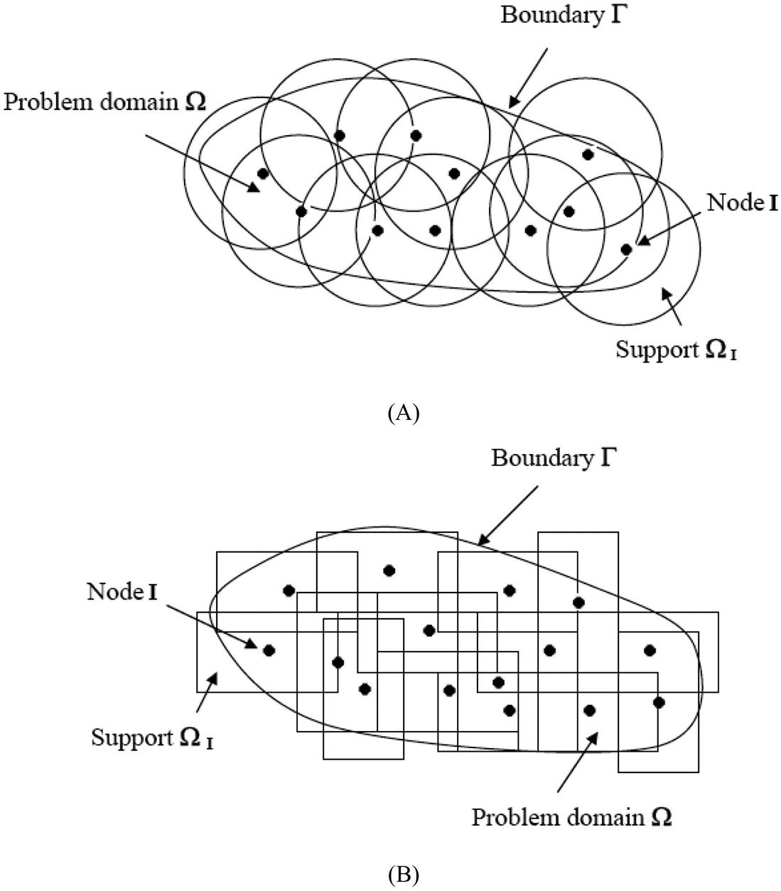
Moreover, mesh-free methods can be viewed as nonlocal approximations, as every evaluated point in the domain is actually covered by the multiple shape functions of the node, as schematically demonstrated in Fig. 4.1. This property may smooth the discontinuous fields and significantly delay the mesh distortion in large deformation computations. It has been found that mesh-free methods can achieve much higher precision levels than the FEM for large deformation problems [85,86,117].
There are several key issues that need to be pointed out here. An important point is the imposition of essential boundary conditions in mesh-free methods. As the mesh-free shape functions generally lack the Kronecker delta property, the approximation generated by the MLS method does not pass through the nodal parameter values. Thus, the essential boundary conditions cannot be enforced as in the FEM. An appropriate technique is needed to impose the essential boundary conditions. Moreover, in the FEM, the integrals can be carried out on a series of discretized elements. However, the concept of elements disappears in mesh-free methods, and the evaluation of the integrals requires the use of certain techniques. The integration method is always an important factor that affects the stability and precision of numerical results. Furthermore, irregular geometrical shapes and irregular boundaries often have an effect on the performance of mesh-free methods and the accuracy of computational results.
4.2 Cauchy–Born Rule
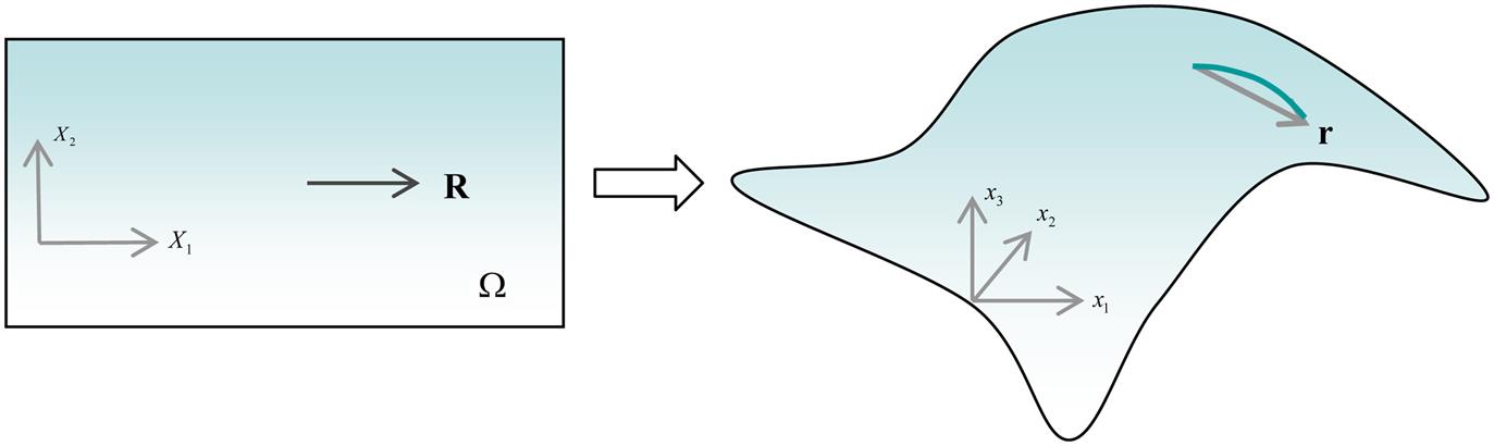
The Cauchy–Born rule [9] is a fundamental kinematic assumption for linking the deformation of the lattice vectors of crystal to that of a continuum deformation field, and it has been applied as a multiscale approach to deal with continuum problems from the viewpoint of the crystal lattice structures. It describes the deformation of crystal lattice vector as:
(4.1)
where r and R are the deformed and undeformed crystal lattice vectors (see Fig. 4.2), and F is the deformation gradient. Arroyo and Belytschko [16–18] argued that this direct application of the standard Cauchy–Born rule may be inaccurate. The application requires sufficiently homogenous deformations mainly because the deformation gradient tensor only maps a tangent vector of the curved surface. A SWCNT is a curved sheet with only one atomic thickness in reality which indicates that the bending effect must be considered. Their computational results also revealed that the bending stiffness based on the standard Cauchy–Born rule is zero. Thus, it cannot truly capture the physical behaviors of CNTs such as buckling behaviors. The approximation can be enhanced by considering the effect of the second-order deformation gradient, and this extended rule is called the higher-order Cauchy–Born rule in the studies of Guo et al. [20] and Wang et al. [21].
From classical nonlinear continuum mechanics [19], the deformed lattice vector r can be expressed as
(4.2)
Taking Taylor’s expansion of the deformation field at S=0, and retaining up to the second-order term, the approximated deformed lattice vector can be derived as
(4.3)
where F and G denote the first- and second-order deformation gradients. With the involvement of the second deformation gradient, the accuracy of approximation for the deformed lattice vectors is largely enhanced. In particular, the second-order deformation gradient can accurately describe the bending stiffness, which makes the results much more reasonable and capable to display the buckling behaviors. Deformation vector r1 obtained by the standard Cauchy–Born rule is linearly dependent on the original vector R and thus stands on the tangent plane of the current configuration. The involvement of the second-order deformation gradient in the higher-order Cauchy–Born rule makes r1 turn towards r2, which is much more approximate to the actual case r (shown in Fig. 4.3).

The simple Bravais lattice possesses the centrosymmetry and the Cauchy–Born rule can be applied directly. Unfortunately, the hexagonal lattice structure in the CNTs is a Bravais multilattice which lacks the centrosymmetry [13–15]. A simple method to solve this problem is decomposing the hexagonal lattice into two simple Bravais sublattices. Under the same deformation, a rigid body translation exists between the two triangular sublattices. Therefore, an internal relaxation η shown in Fig. 4.4 is required to introduce to maintain the minimum potential of atomic system. Eq. (4.3) should be modified as:
(4.4)

Moreover, if we employ an equilibrium graphite sheet as the reference configuration, several additional optimization parameters need be added due to the differences of the bond length and bond angle in the equilibrium graphite sheet and the undeformed CNT.
4.3 Atomistic-Continuum Theory
Based on the higher-order Cauchy–Born rule, an atomistic-continuum theory is derived to simulate the mechanical behaviors of CNTs. In the higher-order deformation gradient theoretical scheme, the strain energy is not only dependent on the first-order deformation gradient, the contribution of the second-order deformation gradient should also be considered. The transformation mapping a three-dimensional curved surface from a two-dimensional planar sheet is described using the higher-order gradient theory. The original planar sheet ![]() and formed curved surface
and formed curved surface ![]() are selected as the reference and current configurations, respectively. Thus, the first- and second-order deformation gradients tensors at point in Eq. (4.4) can be calculated by:
are selected as the reference and current configurations, respectively. Thus, the first- and second-order deformation gradients tensors at point in Eq. (4.4) can be calculated by:
(4.5)
Correspondingly, the first- and second-order stress tensors are [19]:
(4.6)
where ω is the strain energy density and generally determined by the empirical potential in the study of carbon nanostructures in numerical calculation.
The tangential moduli are given by
(4.7)
The higher-order equilibrium equation and Neumann-type boundary conditions are given by:
(4.8)
(4.9)
(4.10)
(4.11)
where ![]() is the body force,
is the body force, ![]() and
and ![]() are the first- and second-order stress tractions on the surface
are the first- and second-order stress tractions on the surface ![]() , N is the outward normal.
, N is the outward normal.
As shown in the hexagonal cellular structure of carbon nanostructures, each carbon atom is connected to three neighboring carbon atoms and we select this atomic structure as the representative cell shown in Fig. 4.5. The chirality is determined by the orientation of this representative cell. The empirical potential for atom I is expressed as:
(4.12)

Since the deformed bond length is a function of the first- and second-order gradient tensors, as well as the inner shift vector shown in Eq. (4.4), the strain energy of atom I can be expressed as:
(4.13)
The area strain energy density can be calculated by:
(4.14)
where ![]() is the average area per atom being
is the average area per atom being ![]() . r0 is the C–C bond length in the initial equilibrium graphite sheet. It is noteworthy that the contribution of the inner shift vector should not be neglected. For a given deformed system, the strain energy should be minimized with respect to the inner shift
. r0 is the C–C bond length in the initial equilibrium graphite sheet. It is noteworthy that the contribution of the inner shift vector should not be neglected. For a given deformed system, the strain energy should be minimized with respect to the inner shift
(4.15)
Therefore, the strain energy density is merely a function of F and G
(4.16)
Consequently, the first- and second-order stress tensors are calculated as
(4.17)
(4.18)
Eqs. (3.40) and (3.41) have clearly demonstrated that the stress tensors are a linear function of the deformation gradient tensors.
The tangential moduli M is evaluated by
(4.19)
(4.20)
(4.21)
(4.22)
Differentiating Eq. (3.38) with respect to the first- and second-order deformation gradient vectors, we have
(4.23)
(4.24)
Thus,
(4.25)
(4.26)
Eqs. (4.17)– (4.22) can be further written as
(4.27)
(4.28)
(4.29)
(4.30)
Matrices grad and σ are defined as a combination of the first- and second-order deformation gradients and stress tensors:
(4.31)
(4.32)
The coordinate of central carbon atom is set as the original point, and the other atoms for the representative cell in the reference configuration and current configuration are denoted as
(4.33)
(4.34)
Consequently, the stress vector can be written as
(4.35)
The tangential moduli is
(4.36)
 (4.36)
![]() in Eq. (4.36) can be obtained by
in Eq. (4.36) can be obtained by
(4.37)
![]() and
and ![]() ,
, ![]() and
and ![]() in Eqs. (4.35)– (4.37) can be determined by the higher-order Cauchy–Born rule Eq. (4.4) and empirical potential Eq. (3.3), respectively. Consequently, the stress vector and tangential moduli can be obtained by being given a deformation description. The developed higher-order deformation gradient theoretical scheme will be used to evaluate the structural and elastic properties of SWCNCs. The whole procedure has been actualized by the developed Fortran program. The constitutive model established based on the higher-order Cauchy–Born rule incorporates the atomic interaction, thus it can accurately display the nonlinear responses of carbon nanostructures under a given deformation description F and G. The buckling and postbuckling behaviors of carbon nanostructures will be discussed in detail in the later numerical simulations.
in Eqs. (4.35)– (4.37) can be determined by the higher-order Cauchy–Born rule Eq. (4.4) and empirical potential Eq. (3.3), respectively. Consequently, the stress vector and tangential moduli can be obtained by being given a deformation description. The developed higher-order deformation gradient theoretical scheme will be used to evaluate the structural and elastic properties of SWCNCs. The whole procedure has been actualized by the developed Fortran program. The constitutive model established based on the higher-order Cauchy–Born rule incorporates the atomic interaction, thus it can accurately display the nonlinear responses of carbon nanostructures under a given deformation description F and G. The buckling and postbuckling behaviors of carbon nanostructures will be discussed in detail in the later numerical simulations.
4.4 Structural and Elastic Properties of SWCNTs
4.4.1 Transformation of SWCNTs
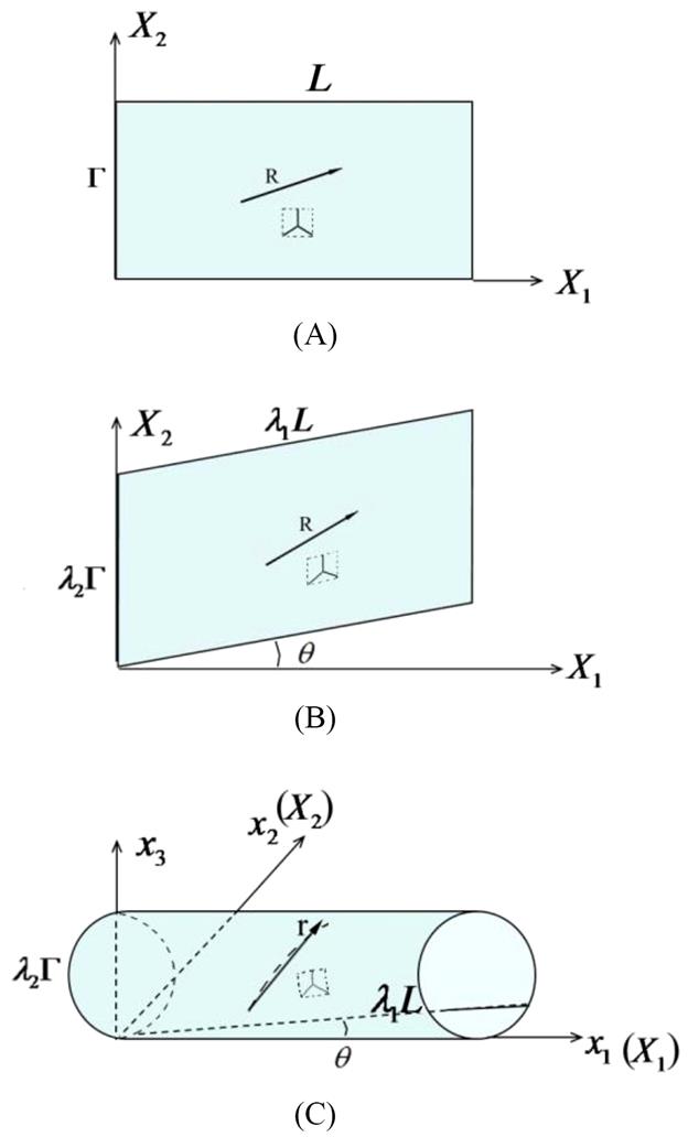
An undeformed SWCNT can be considered as the rolling up of an initial equilibrium graphite sheet into a hollow cylindrical structure. It is noteworthy that the atomic structure of an initial equilibrium graphite sheet is different from that of an initial equilibrium SWCNT. All of the C–C bonds are the same in the initial equilibrium graphite sheet, while there are slight differences in C–C bonds in the counterpart SWCNT. Therefore, three geometrical parameters, λ1, λ2, and θ, corresponding to the uniform longitudinal, circumferential stretches, and the skew of any surface longitudinal line, respectively, are introduced to describe this shifting process. The three geometrical parameters can be determined by minimizing the strain energy of the representative cell to obtain an initial equilibrium configuration. The initial equilibrium graphite sheet and the optimized equilibrium SWCNT are selected as the reference configuration and the current configuration, respectively. The deformation process mapped from Fig. 4.6A–C can then be written:
(4.38)
(4.39)
(4.40)
where ![]() and
and ![]() are the current configuration and reference configuration, respectively. The first- and second-order deformation gradients F and G can be exactly calculated from the deformation process of SWCNTs in Eqs. (4.38)– (4.40).
are the current configuration and reference configuration, respectively. The first- and second-order deformation gradients F and G can be exactly calculated from the deformation process of SWCNTs in Eqs. (4.38)– (4.40).
When the three parameters λ1, λ2, and θ are introduced, the first- and second deformation gradients are determined by the three parameters and Eq. (4.14) can be further rewritten as:
(4.41)
Denote the unknown vector as:
(4.42)
Structural parameters can be determined by minimizing the strain energy of the representative cell:
(4.43)
The Taylor expansion of ![]() around an initial guess of
around an initial guess of ![]() for the equilibrium state is
for the equilibrium state is
(4.44)
Substitution of Eq. (4.44) into (4.43) yields the following governing equation
(4.45)
The increment of structural vector ![]() can be determined by iteratively solving Eq. (4.45) until the right term reaches zero.
can be determined by iteratively solving Eq. (4.45) until the right term reaches zero.
The aforementioned strain energy density ![]() in Eq. (4.14) is defined as the area strain energy density, while the volume strain energy density is required in order to calculate the elastic and structural properties. Nevertheless, there is no agreed thickness concept for CNTs. Scholars have suggested an interlayer distance of approximately 0.33~0.34 nm for CNTs. In many publications [118,119], the interlayer distance of graphite sheet is chosen as 0.334 nm, hence we choose it as the thickness. Consequently, the volume strain energy density is calculated by:
in Eq. (4.14) is defined as the area strain energy density, while the volume strain energy density is required in order to calculate the elastic and structural properties. Nevertheless, there is no agreed thickness concept for CNTs. Scholars have suggested an interlayer distance of approximately 0.33~0.34 nm for CNTs. In many publications [118,119], the interlayer distance of graphite sheet is chosen as 0.334 nm, hence we choose it as the thickness. Consequently, the volume strain energy density is calculated by:
(4.46)
where t is the thickness.
Since geometrical parameters λ1 and λ2 correspond to the uniform axial and circumferential stretches, respectively, the axial and circumferential strains are calculated by:
(4.47)
Thus, axial and circumferential stresses are determined by:
(4.48)
In case of hydrostatic pressure, CNTs deform uniformly along the circumference. The radial strains of the CNTs equal the circumferential strains, i.e., ![]() . Moreover, the hydrostatic pressure p has a relationship with
. Moreover, the hydrostatic pressure p has a relationship with ![]() as
as
(4.49)
Young’s moduli along the axial and circumferential directions of CNTs E1 and E2 can be obtained by:
(4.50)
 (4.50)
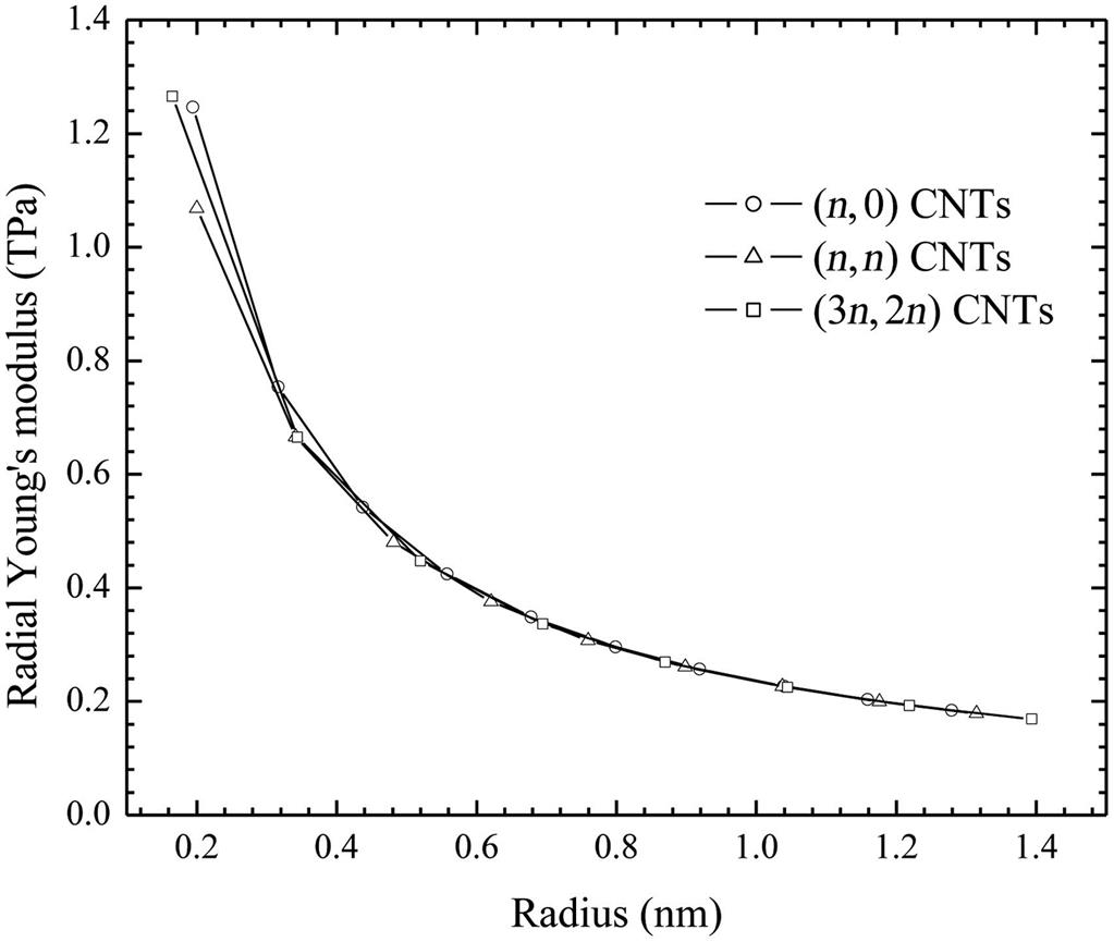
Using Eq. (4.49), the radial Young’s modulus can be calculated as
(4.51)
The angle θ is the shear strain at the surface and thus the shear stress at the cross-section is:
(4.52)
The shear modulus is calculated by:
(4.53)
The Poisson’s ratio is calculated by:
(4.54)
Moreover, we have the relationship
(4.55)
Similar to the calculation of tangential modulus, it is noteworthy that the contribution of the inner shift vector should not be neglected when calculating elastic constants. Structural parameters of CNTs can be obtained by iteratively solving the incremental governing equation Eq. (4.45), and elastic properties are the values of Eqs. (4.50)– (4.54) at the initial equilibrium state of CNTs.
4.4.2 Structural Parameters
With the solution of Eq. (4.45), the structural parameters of the initial undeformed SWCNT can be obtained. Here, the second set of parameters [120] for the Brenner potential is employed. In the calculation, we need to present a number as the initial bond length for the representative cell in the reference graphite sheet (Fig. 4.7A). Essentially, we can choose any number as the initial optimization value, and the choice of this value has no effect on the final optimized results. Moreover, by setting a very large tube radius, we can obtain the bond length in the initial equilibrium graphite sheet. For the second set of parameters of the Brenner potential, our computation indicates that the bond length in the initial equilibrium graphite sheet is 0.14507 nm which is used as the initial value of the bond lengths in the reference configuration. With this choice, the evaluated values of λ1, λ2, and θ are, respectively, the axial and circumferential stretches and twisting angle of the tube relative to the initial equilibrium graphite sheet.
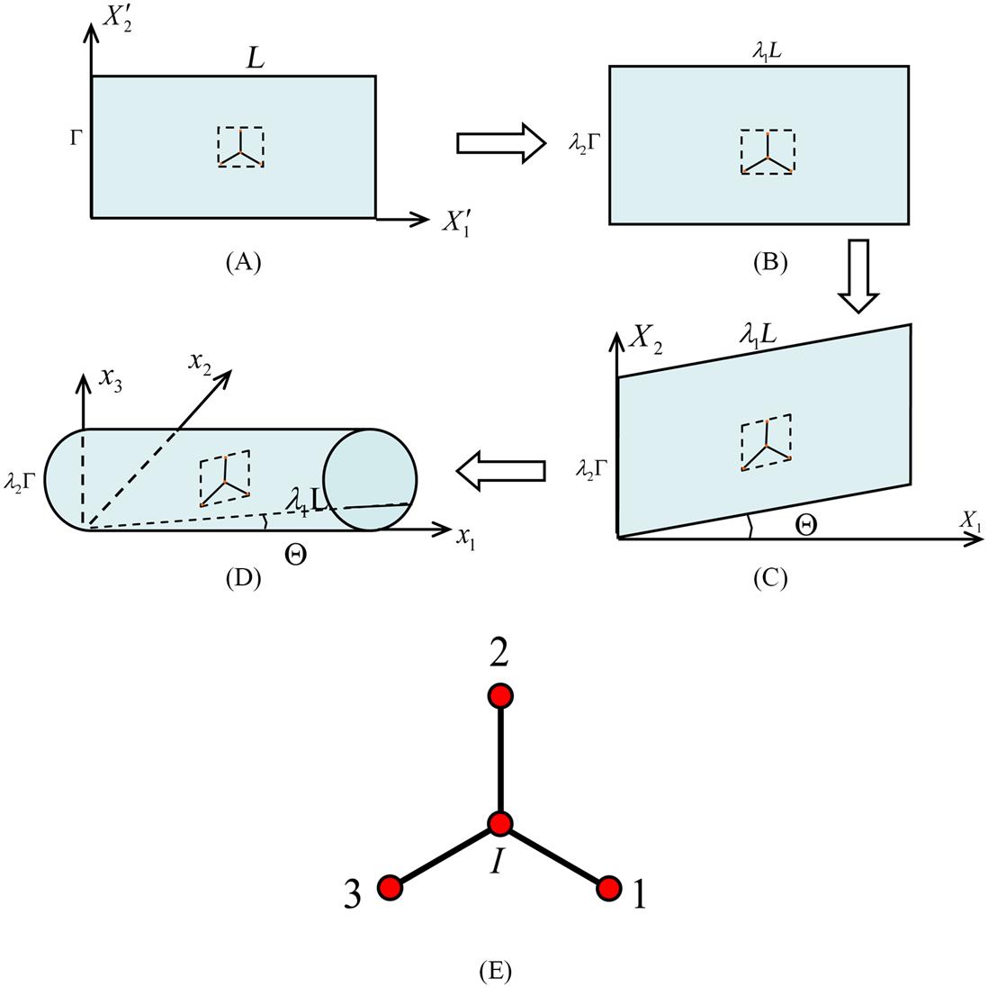
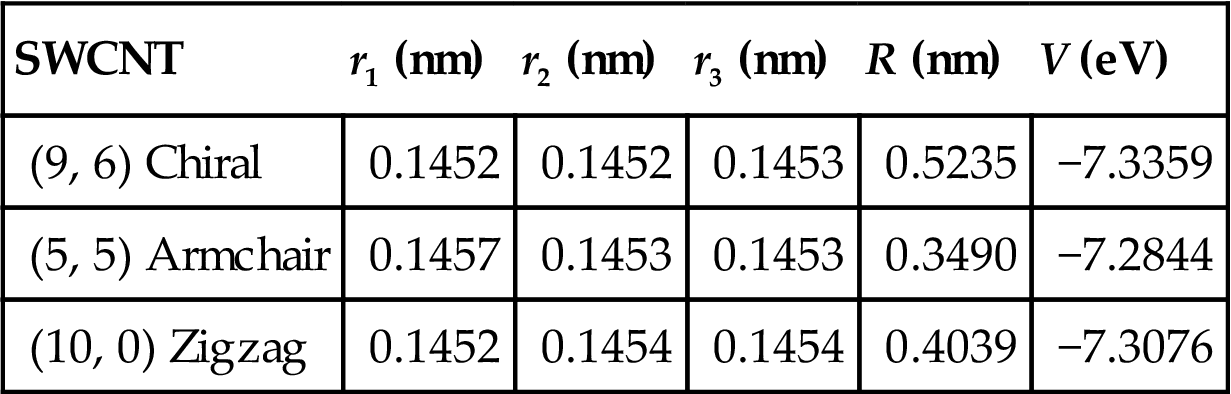
Table 4.1 shows the evaluated values of λ1, λ2, and θ for chiral (9, 6), armchair (5, 5), and zigzag (10, 0) SWCNTs. It is noted that θ=0 for the armchair and zigzag SWCNTs, whereas a nonzero twisting angle θ occurs for the chiral CNT. This is because the representative cells in the armchair and zigzag CNTs are axisymmetric with respect to the axial and circumferential directions of the tube. The evaluated bond lengths and tube radii are listed in Table 4.2, along with the calculated atomic energy. Table 4.3 gives the results obtained by Chandraseker and Mukherjee [121]. The present results for bond lengths and atomic energy display excellent agreement with those of Chandraseker and Mukherjee [121]. However, the tube radius shows a slight discrepancy, and this may be because of a difference in the radius definitions in the two methods. (9, 6), (5, 5), and (10, 0) SWCNTs belong to tubes of small radius. The present computations show that the approximation with the first- and second-order deformation gradient is precise enough even for tubes of small radius.
Table 4.1
Optimization Values for λ1, λ2, and θ [24]
| SWCNT | λ1 | λ2 | θ (°) |
| (9, 6) Chiral | 1.00100 | 0.99411 | 0.08554 |
| (5, 5) Armchair | 1.00307 | 0.98606 | 0 |
| (10, 0) Zigzag | 0.99820 | 0.99346 | 0 |
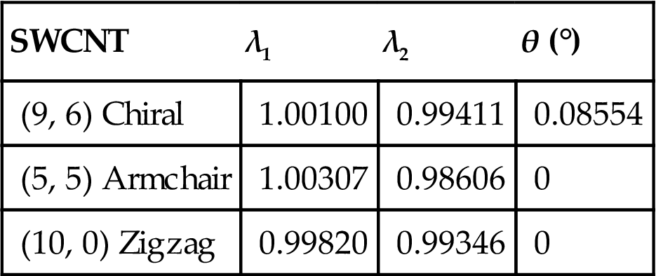
Table 4.2
Bond Lengths, Tube Radius, and Atomic Energy in the Undeformed SWCNTs Obtained With the Present Method [24]
| SWCNT | r1 (nm) | r2 (nm) | r3 (nm) | R (nm) | V (eV) |
| (9, 6) Chiral | 0.14520 | 0.14516 | 0.14533 | 0.51986 | −7.33606 |
| (5, 5) Armchair | 0.14567 | 0.14532 | 0.14532 | 0.34150 | −7.28637 |
| (10, 0) Zigzag | 0.14518 | 0.14544 | 0.14544 | 0.39729 | −7.30785 |
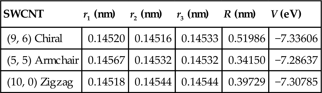
Table 4.3
Bond Lengths, Tube Radius, and Atomic Energy in the Undeformed SWCNT in Ref. [121]
| SWCNT | r1 (nm) | r2 (nm) | r3 (nm) | R (nm) | V (eV) |
| (9, 6) Chiral | 0.1452 | 0.1452 | 0.1453 | 0.5235 | −7.3359 |
| (5, 5) Armchair | 0.1457 | 0.1453 | 0.1453 | 0.3490 | −7.2844 |
| (10, 0) Zigzag | 0.1452 | 0.1454 | 0.1454 | 0.4039 | −7.3076 |
4.4.3 Elastic Properties
Computations have been carried out for different types of CNTs. In the results analysis, we use (3n, 2n) CNTs as an example to illustrate the properties of chiral CNTs. In all of the calculations, the first- and second-order derivatives are exactly computed. Fig. 4.8 shows the variation of the axial and circumferential Young’s moduli with the tube radius. With an increasing tube radius, the axial and circumferential Young’s moduli trend to the same constant that corresponds to the Young’s modulus of the graphite sheet. The present estimated value is 0.7049 TPa, which is very close to that predicted by Arroyo and Belytschko [18]. When the tube radius is larger than 0.5 nm, the moduli are very close to those of the graphite sheet, and the maximum difference is less than 2%. Moreover, we also notice a special phenomenon: the axial and circumferential Young’s moduli of the CNTs are generally less than those of the graphite sheet, but the circumferential Young’s moduli of the zigzag CNTs are slightly larger than those of the graphite sheet. This indicates that the chirality of CNTs has an effect on their properties, but this effect is very slight when the tube radius is larger than 0.5 nm. Plotted in Fig. 4.9 is the radial Young’s modulus versus the tube radius. The radial Young’s modulus has a large dependence on the tube radius, because it is equal to the circumferential Young’s modulus divided by the tube radius. Fig. 4.10 shows the variation of Poisson’s ratio ![]() with the tube radius. Similar to the axial and circumferential Young’s moduli,
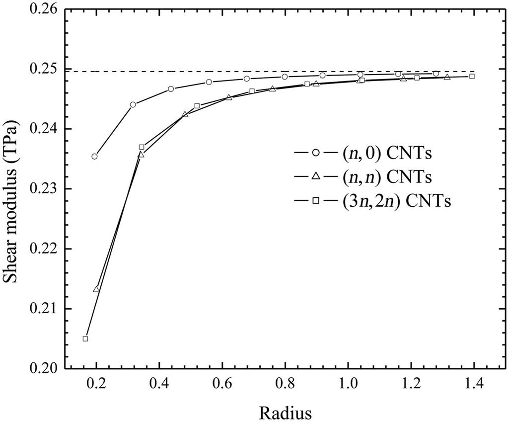
with the tube radius. Similar to the axial and circumferential Young’s moduli, ![]() trends to the Poisson’s ratio of the graphite sheet (the present estimated value is 0.4123). When the tube radius is larger than 0.5 nm, the Poisson’s ratio is very close to 0.4123. Fig. 4.11 shows the dependence of the shear modulus on the tube radius. When the tube radius is larger than 0.5 nm, the shear modulus is very close to that of the graphite sheet. The present estimated shear modulus of the graphite sheet is approximately 0.25 TPa. In conclusion, the elastic properties of CNTs have a dependence on the chirality and the tube radius, but when the tube radius is larger than 0.5 nm, the axial and circumferential Young’s moduli, Poisson’s ratio, and shear modulus are pretty close to those of the graphite sheet. Therefore, CNTs can be viewed as a curved surface on which the elastic properties at the tangent direct are almost the same with the graphite sheet.
trends to the Poisson’s ratio of the graphite sheet (the present estimated value is 0.4123). When the tube radius is larger than 0.5 nm, the Poisson’s ratio is very close to 0.4123. Fig. 4.11 shows the dependence of the shear modulus on the tube radius. When the tube radius is larger than 0.5 nm, the shear modulus is very close to that of the graphite sheet. The present estimated shear modulus of the graphite sheet is approximately 0.25 TPa. In conclusion, the elastic properties of CNTs have a dependence on the chirality and the tube radius, but when the tube radius is larger than 0.5 nm, the axial and circumferential Young’s moduli, Poisson’s ratio, and shear modulus are pretty close to those of the graphite sheet. Therefore, CNTs can be viewed as a curved surface on which the elastic properties at the tangent direct are almost the same with the graphite sheet.


4.4.4 Pressure–Radial Strain Curve
The above method can be viewed as an analytical-numerical method, in which the first- and second-order derivatives of the strain energy density are calculated exactly, and Newton’s method is used only to determine the minimum point of energy. Moreover, by varying the values of λ1, λ2, and θ, and then minimizing the energy density, we can calculate the mechanical response of CNTs under axial tension or compression (varying λ1), hydrostatic pressure (varying λ2), and twisting (varying θ). This method can also be used to study the interaction of different loading conditions, e.g., the twisting behavior of different chiralities of CNTs under axial or radial compression. Here, the hydrostatic pressure–radial strain and axial strain–stress curves are presented as two examples.
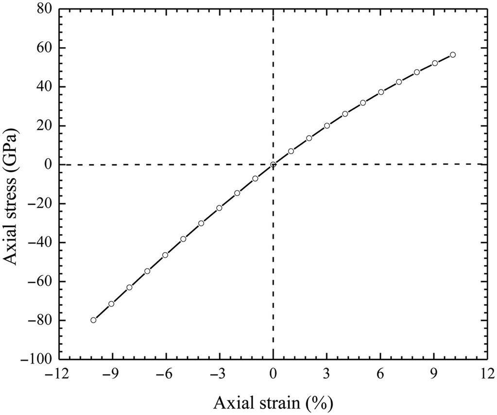
The axial strain–stress curves of SWCNTs can be obtained by varying the value of λ1. For a given λ1 that corresponds to an axial strain, the energy minimization results in the values of λ2 and θ and the axial stress can be calculated using Eq. (4.48). By varying λ1, the axial strain–stress can be obtained. Plotted in Fig. 4.12 is the axial strain–stress curve of a (15, 0) SWCNT.
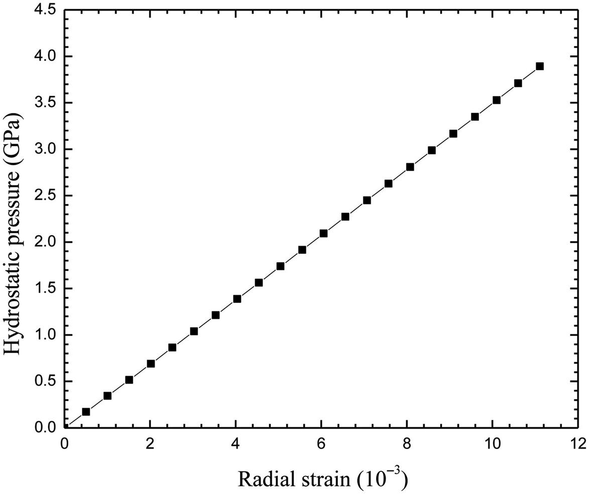
The pressure–radial strain curve of SWCNTs under hydrostatic pressure can be obtained by varying the value of λ2. For a given λ2 that corresponds to a radial compressive strain, energy minimization gives the values of λ1 and θ, and the hydrostatic pressure can be calculated as ![]() . By varying λ2, the curve of the hydrostatic pressure versus the radial strain (λ2−1) can be obtained. Plotted in Fig. 4.13 is the pressure–radial strain curve of a (10, 10) SWCNT.
. By varying λ2, the curve of the hydrostatic pressure versus the radial strain (λ2−1) can be obtained. Plotted in Fig. 4.13 is the pressure–radial strain curve of a (10, 10) SWCNT.
4.5 Mesh-Free Computational Framework
Before deriving a mesh-free formulation for SWCNTs, we need to discuss the establishment of the appropriate reference configuration and the determination of the structure of the representative cell in the reference configuration. In the previous analysis, we use three geometric parameters λ1, λ2, and θ to define a transformation from a planar graphite sheet to an undeformed SWCNT. The computations show that this rolling is not a simple grid transformation and that the atomic structure readjusts to attain the minimum system energy during the rolling process. In the numerical simulations, we need to consider the transformation from the reference configuration to the deformed configuration (the current configuration). For an arbitrary given deformation description (deformation gradients F and G), we need to determine the constitutive response of the system (the stress tensors P and Q and the modulus M), and these three geometrical parameters no longer have a clear physical meaning. We should find an appropriate planar sheet structure as the reference configuration so that the transformation from this sheet to the initial equilibrium SWCNT is a rigid map. From the previous analysis, it can be seen that Fig. 4.7C is such a sheet.
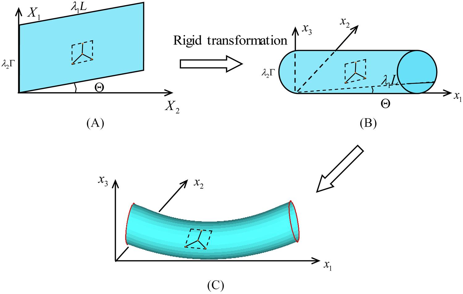
In the future numerical simulations, we use Fig. 4.7C as the reference configuration. Thus, the deformation from the reference configuration to the deformed SWCNT can be divided into two steps (see Fig. 4.14): one is from the reference configuration to the initial equilibrium SWCNT, and the other is from the initial equilibrium SWCNT to the current configuration. The first step can be exactly expressed as
(4.56)
 (4.56)
Eq. (4.56) also maps the cell structure in the reference configuration to that in the initial SWCNT by minimizing the energy of the cell structure with only the inner shift being used as the optimization parameter. The cell structure in the reference configuration can be determined with the method described in Section 4.4.1. This cell structure is the original image of the representative cell.
The transformation map from the reference configuration to the current configuration is
(4.57)
 (4.57)
where u1, u2, and u3 are the displacements of an SWCNT relative to its undeformed counterpart (Fig. 4.14B), whereas Eq. (4.56) denotes the first step of the deformation of an SWCNT (the reference configuration to the initial SWCNT), u1, u2, and u3 describe the remaining step (from the initial SWCNT to the current configuration), which is numerically computed in the later mesh-free numerical simulations. To determine the cell structure at any point of the current configuration, the energy of the cell structure is minimized only with respect to the inner shift. Such a minimizing algorithm also gives the results of the stresses and tangent modulus with the application of the formulas (4.35) and (4.36).
In mesh-free methods, the problem domain is discretized by a set of nodes, and each node has compact supports (shown in Fig. 4.1). For a 2-D domain, the two basic support types are discs and rectangles. The mesh-free nodes are collocated on the reference configuration, and the displacement u1, u2, and u3 is interpolated with the mesh-free nodal parameters. As the transformation from the reference configuration to an undeformed SWCNT is a simple grid mapping, the mesh-free nodes can also be viewed as having been collocated on the surface of the undeformed SWCNT. Fig. 4.15 shows a node collocation on an undeformed SWCNT.

Mesh-free shape functions are always one of the key points in the development of mesh-free methods. The present research introduces two interpolation methods in detail, i.e., MLS approximation and moving Kriging interpolation, to construct the mesh-free shape function, and discusses their basic properties that are relative to the future application.
4.5.1 Moving least-squares approximation
In the MLS approximation, any variable ![]() that is defined in a domain
that is defined in a domain ![]() can be approximated by
can be approximated by ![]() in the subdomain
in the subdomain ![]() , as follows.
, as follows.
(4.58)
where ![]() is the monomial basis function, m is the number of terms in the basis, and
is the monomial basis function, m is the number of terms in the basis, and ![]() are the coefficients of the basis function. The commonly used basis is the linear basis
are the coefficients of the basis function. The commonly used basis is the linear basis
(4.59)
(4.60)
and the quadratic basis is
(4.61)
(4.62)
Certain basis functions can be used to satisfy the special properties of the variable. For example, the following basis function can capture stress singularity in linear-elastic fracture mechanics [116].
(4.63)
where r and θ are polar coordinates with the crack tip as the origin.
The unknown coefficients ![]() in Eq. (4.58) can be determined by the minimization of the weighted discrete L2 norm as
in Eq. (4.58) can be determined by the minimization of the weighted discrete L2 norm as
(4.64)
where ![]() is the weight function with compact support, and NP is the number of nodes with
is the weight function with compact support, and NP is the number of nodes with ![]() . The minimum of J in Eq. (4.64) with respect to
. The minimum of J in Eq. (4.64) with respect to ![]() leads to a set of linear equations:
leads to a set of linear equations:
(4.65)
where ![]() , and
, and
(4.66)
and
(4.67)
Thus, the unknown coefficients ![]() can be obtained from Eq. (4.64) as
can be obtained from Eq. (4.64) as
(4.68)
Substituting Eq. (4.68) into Eq. (4.58), the MLS approximation can be written in standard form as
(4.69)
where the MLS shape function ![]() is defined as
is defined as
(4.70)
The partial derivatives of ![]() with respect to XK can be obtained as
with respect to XK can be obtained as
(4.71)
in which
(4.72)
(4.73)
(4.74)
The second partial derivatives of ![]() are obtained as
are obtained as
(4.75)
in which
(4.76)
(4.77)
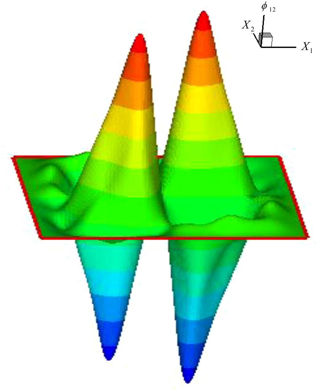
In the present research, the quadratic basis (Eq. 4.62) is used, and the weight function is chosen as the cubic spline function (Eq. 4.80). Shown in Fig. 4.16 is a plot of the MLS shape function. Fig. 4.16A presents the 2-D view, and Fig. 4.16B the variation of the shape function along the X1 direction (X2=0), which corresponds to the 1-D MLS shape function. Fig. 4.17 shows the first-order derivative of the shape function ![]() , and plotted in Figs. 4.18 and 4.19 are the second-order derivatives
, and plotted in Figs. 4.18 and 4.19 are the second-order derivatives ![]() and
and ![]() .
.
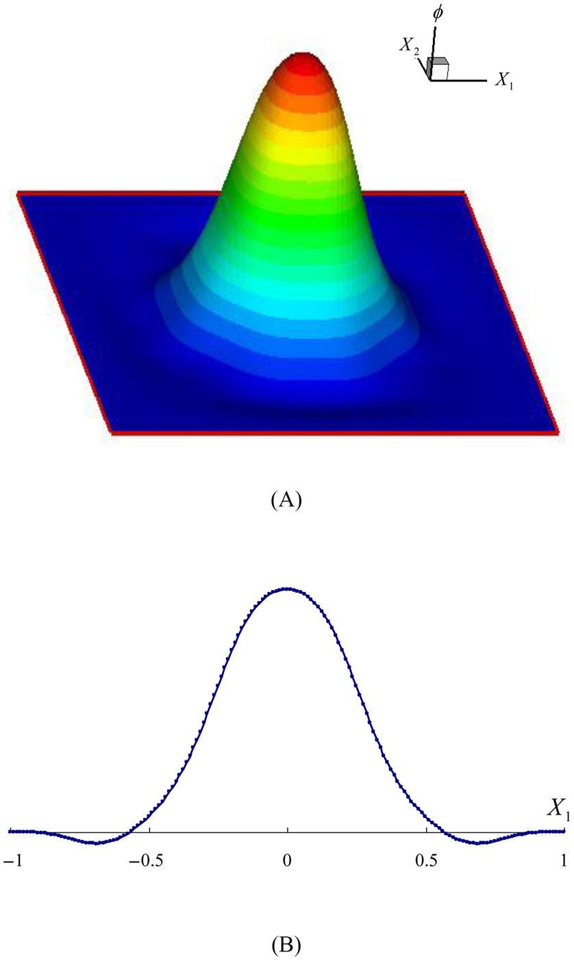
 constructed on the 2-D domain; (B) the variation of along the X1 direction (X2=0).
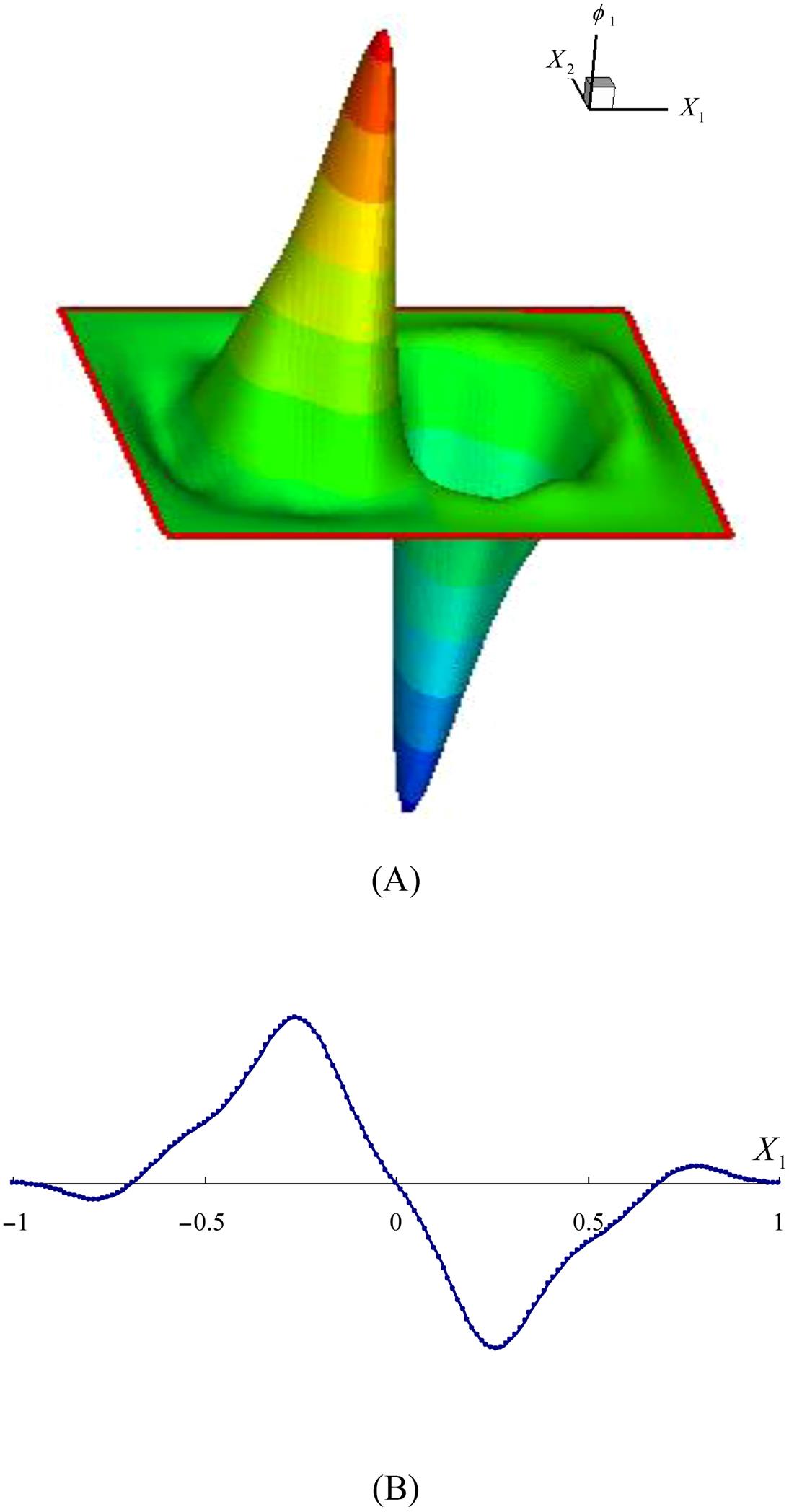 of the mesh-free shape function constructed on a 2D domain; (B) the variation of along the X1 direction (X2=0).
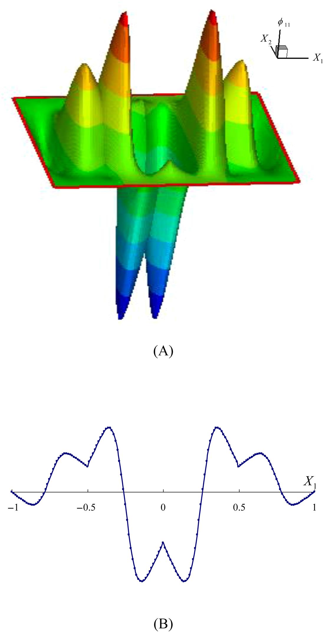


4.5.2 Weight Functions
The choice of weight functions is an important ingredient in mesh-free methods, as these functions affect the continuity and accuracy of the resulting mesh-free approximation. Generally, the weight functions can result in C2 or higher-order continuity of the shape functions. To generate a set of sparse discrete equations, the weight functions are defined as having a compact support, which means that they should be nonzero only over a small neighborhood of node XI.
The commonly used weight functions are in the following forms.
(4.78)
(4.79)
 (4.79)
(4.80)
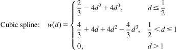 (4.80)
(4.81)
where d is the normalized distance, and α is a dilation parameter of the weight function.
In the 1-D case, the weight function is written as
(4.82)
where ![]() , and cI is the size of the support of node XI.
, and cI is the size of the support of node XI.
In the 2-D case, there are two commonly used supports. For the circular compact support shown in Fig. 4.1A, the weight function can be written as
(4.83)
where ![]() , and RI is the radius of the support of node XI.
, and RI is the radius of the support of node XI.
For the rectangular compact support shown in Fig. 4.1B, the product weight function is given by
(4.84)
where ![]() ,
,![]() , and
, and ![]() is the size of the rectangular support of node XI.
is the size of the rectangular support of node XI.
The MLS approximation is closely related to the weight functions and the basis functions. Dolbow and Belytschko [122] stated that if the continuity of the basis function is greater than the continuity of the weight function, then the resulting approximation would inherit the continuity of the weight function. The exponential weight can resemble a weight with C1 or higher-order continuity. The cubic and quartic weights possess C2 continuity, which is ideal for constructing the mesh-free shape function with C2 continuity.
4.5.3 Domain of Influence of Nodes
The weight functions are defined as having a compact support, i.e., the subdomain over it is nonzero. Each subdomain ![]() is associated with a node
is associated with a node ![]() , which can be termed the node’s domain of influence (DOI). The way in which the DOI for each node is determined has a tremendous impact on the total performance of a mesh-free method. The node’s DOI is inherent in the weight function’s compact support, which makes the interpolation limited on the several nodes whose supports cover the evaluated point. The most commonly used supports for 2-D problems are circular and rectangular supports, as shown in Fig. 4.1. The shape of the support has almost no effect on the results.
, which can be termed the node’s domain of influence (DOI). The way in which the DOI for each node is determined has a tremendous impact on the total performance of a mesh-free method. The node’s DOI is inherent in the weight function’s compact support, which makes the interpolation limited on the several nodes whose supports cover the evaluated point. The most commonly used supports for 2-D problems are circular and rectangular supports, as shown in Fig. 4.1. The shape of the support has almost no effect on the results.
In the 1-D case, the size of the support can be defined as
(4.85)
where ![]() is a scaling factor, and
is a scaling factor, and ![]() is the basic support of node
is the basic support of node ![]() .
. ![]() can be determined by the maximum distance to its nearest neighboring node.
can be determined by the maximum distance to its nearest neighboring node.
The radius of the circular support can be defined as
(4.86)