
Technologically Relevant Applications
Abstract
Carbon nanotubes (CNTs) hold significant promise for potential applications such as fluid transport, fluid storage, biosensors, and drug-delivery devices, in view of their perfect hollow cylindrical structure and superior elastic properties. In this chapter, the possibility of fluid flow measurement in fluid-conveying single-walled CNTs (SWCNTs) is investigated using the free vibration analysis. Molecular dynamics (MD) simulation is performed to investigate how the methane molecules manipulate the transport of water molecules through SWCNTs and diameter-gradient SWCNTs with junctions. MD simulation is also carried out for a systematic study of the adsorption process of hydrogen atoms onto the (5, 5) CNT sidewall. Finally, according to the high fundamental frequencies of carbon nanocones, their application in highly sensitive mass detection is investigated.
Keywords
Conveying fluid; driving water molecules; hydrogen storage; mass detection
8.1 Introduction
Carbon nanotubes (CNTs) hold significant promise for potential applications such as fluid transport, fluid storage, biosensors, and drug-delivery devices, in view of their perfect hollow cylindrical structure and superior elastic properties. CNTs offer high diffusion coefficients for liquids as well as gases due to the natural smoothness of their inner walls [1–5]. The simulations and experimental results in recent years have proven that the molecular transport through CNTs is far in excess of what is predicted by continuum hydrodynamics theories [6–9]. Studies of the elastic properties of CNTs are numerous in the literature, whereas studies on fluid conveying CNTs [3,6,8,10–12] and fluid flow around CNTs [13,14] are relatively scarce. The behavior of the fluid inside CNTs is expected to be fundamentally different from the behavior of the fluid in macro/microsystems at low velocities because of the very small diameter of CNTs, and therefore it offers itself as a significant and challenging research topic in nanoelectromechanical systems (NEMS) [10,15]. Dynamic analysis has been conducted by researchers to study the behavior of CNTs under a wide range of fluid flow velocities from 0 to 100,000 m/s using elastic beam models and molecular dynamics (MD) simulations [8,10,11,16]. The simulations give insight into the direction of fluid flow measurements in single-walled CNTs (SWCNTs).
Water molecules confined in nanoscale pores usually have different transport behaviors from those of bulk system [17–21]. The molecular transport in nanoporous media raises many interesting theoretical problems [22]. Understanding the transport of water molecules through CNT is an important practical issue in biological science [23–28], because the transport behavior of water through CNT is very similar to the flow of water in the cellular membrane of biological systems. Hummer and coworkers [19] observed the spontaneous and continuous filling of CNT with a one-dimensional ordered chain of water. Joseph and Aluru [29] used MD simulation to investigate water flow through different types of tubes and showed that the enhanced flow rate was due to the smooth surface of the nanotube. Rossi et al. [30] studied the flow and condensation of water inside CNT by means of environmental scanning electron microscopy (SEM). He suggested that the slow flow of liquid is a result of the confinement of water and its strong interaction with tube walls. Although much progress has been achieved in both the theoretical and experimental studies on the nanofluidic properties of water through CNTs, some fundamental questions like the nano-hydromechanics of water flow through CNTs remain unanswered. Hence, it is valuable to design a functional device [31,32] to control the transport of water molecules through CNTs. Pressure gradients were imposed on a nanoscale system to drive the water transport through CNTs [33], where pressure difference of two ends of SWCNT is up to 60 atm. Zambrano et al. [34] used thermal gradients to induce water transport through SWCNTs, in which the temperature difference imposed on two ends of SWCNT reached up to 140K. High pressure and temperature gradient imposed on the given systems would change the physical and chemical properties of water (even phase transition), which affect the accuracy of the research results. Electric current applied to the SWCNT is a good method to drive water flow through nanotubes [35]. However, this experiment is difficult to perform because the required apparatus is complicated. Moreover, the water molecules are possible to be electrolyzed by electric current. Manipulation of the flow of water molecules through CNTs is a challenging issue. Until now, this issue has not been well tackled. Few research results have been reported on the transport of water molecules driven by methane molecules.
In this chapter, the possibility of fluid flow measurement in fluid-conveying SWCNTs is investigated using the free vibration analysis. MD simulation is performed to investigate how the methane molecules manipulate the transport of water molecules through SWCNTs and diameter-gradient SWCNTs with junctions.
8.2 Conveying Fluid
The free vibration analysis of fluid-conveying SWCNTs is performed by assuming a frictionless contact between the fluid and SWCNT wall. The objective is to examine the effects of an internal moving fluid on the free vibration natural frequency, mode shape, and various forces, i.e., stiffness, inertia, Coriolis, and centrifugal, as well as the structural instability of SWCNTs.
The SWCNT in the present analysis is treated as a perfect hollow cylindrical tube having an equivalent bending rigidity EI with a mass mc per unit length, as shown in Fig. 8.1. Let ![]() be the uniform mean flow velocity of the fluid and mf be the mass of fluid per unit length of the SWCNT. The governing differential equation of motion for the fluid conveying tube can be expressed as [37]
be the uniform mean flow velocity of the fluid and mf be the mass of fluid per unit length of the SWCNT. The governing differential equation of motion for the fluid conveying tube can be expressed as [37]
(8.1)
where the four terms on the left side correspond to the inertial, Coriolis/gyroscopic, centrifugal, and stiffness forces, respectively, the last term is entirely related to the structure SWCNT, the second and third terms are entirely related to the fluid flow, while the first term is related to both structure and fluid. The bending rigidity EI in Eq. (8.1) is an input parameter for a given fluid and size of a SWCNT. One needs to know the exact values of Young’s modulus and wall thickness of a SWCNT to compute the bending rigidity. It is unclear as to how one can choose appropriate values in view of wide scattered data reported in the literature. Hence, a different approach is followed here: an equivalent bending rigidity is computed instead of using the assumed values of Young’s modulus and wall thickness from literature. The stiffness matrix of the SWCNT is first computed using the finite difference method. Next, a free vibration analysis is performed using the obtained stiffness matrix and the lumped mass matrix of carbon atoms to compute the fundamental natural frequencies, where the mass of the fluid is set to be zero in Eq. (8.1). The relationship between the fundamental natural frequency f and the bending rigidity EI can be expressed as ![]() for a fixed–fixed SWCNT, where β=1.506π for the fundamental mode. The bending rigidity is therefore obtained as
for a fixed–fixed SWCNT, where β=1.506π for the fundamental mode. The bending rigidity is therefore obtained as ![]() . The computed EI values for various diameters of SWCNTs are listed in Table 8.1.
. The computed EI values for various diameters of SWCNTs are listed in Table 8.1.

Table 8.1
μ1 Computed Bending Rigidity Values for SWCNTs [36]
| SWCNT Type | Diameter (nm) | Bending Rigidity EI (N·m2) |
| (5, 0) | 0.415 | 4.7102×10⁻²⁷ |
| (8, 0) | 0.65 | 1.9770×10⁻²⁶ |
| (12, 0) | 0.961 | 7.7374×10⁻²⁶ |
| (14, 0) | 1.12 | 1.1122×10⁻²⁵ |
| (16, 0) | 1.28 | 1.6867×10⁻²⁵ |
Eq. (8.1) represents a linear homogeneous system that can be solved for eigenvalues and eigenvectors by recasting it into an equivalent state–space form. The computed natural frequencies depend on the size of the SWCNT and the mass flow rate of the fluid. Nondimensional parameters, i.e., the mass ratio mr and the dimensionless velocity vn are introduced for convenience, i.e., ![]() and
and ![]() . The natural frequencies of the fluid conveying SWCNT are computed by varying these nondimensional parameters. The fluid being conveyed is assumed to be water. It is also assumed that no fluid is outside the SWCNT. The approach presented here is not limited to water-conveying SWCNTs and can be extended to any fluid. Fig. 8.2 shows the variation of the natural frequency with respect to the dimensionless velocity of the fluid for the lowest three natural modes of a fluid conveying SWCNT. The computed values of the first, second, and third frequencies at zero velocity of the fluid are
. The natural frequencies of the fluid conveying SWCNT are computed by varying these nondimensional parameters. The fluid being conveyed is assumed to be water. It is also assumed that no fluid is outside the SWCNT. The approach presented here is not limited to water-conveying SWCNTs and can be extended to any fluid. Fig. 8.2 shows the variation of the natural frequency with respect to the dimensionless velocity of the fluid for the lowest three natural modes of a fluid conveying SWCNT. The computed values of the first, second, and third frequencies at zero velocity of the fluid are ![]() , and
, and ![]() respectively. The centrifugal force increases and the resultant stiffness decreases as the velocity of the fluid increases, this is because the centrifugal force acts in the opposite direction to the stiffness force, and as a result the natural frequencies decrease with an increase in the fluid velocity. The dimensionless velocity at which the fundamental natural frequency becomes zero is defined as the critical velocity
respectively. The centrifugal force increases and the resultant stiffness decreases as the velocity of the fluid increases, this is because the centrifugal force acts in the opposite direction to the stiffness force, and as a result the natural frequencies decrease with an increase in the fluid velocity. The dimensionless velocity at which the fundamental natural frequency becomes zero is defined as the critical velocity ![]() and is equal to 2π, as shown in Fig. 8.2. The structure is unstable at this velocity because the resultant stiffness is zero.
and is equal to 2π, as shown in Fig. 8.2. The structure is unstable at this velocity because the resultant stiffness is zero.

The magnitudes of inertial, Coriolis, centrifugal, and stiffness forces are computed along the length of the SWCNT at various fluid velocities. The distribution of these forces normalized with respect to the stiffness force is plotted against the nondimensional length of the SWCNT, as shown in Fig. 8.3 at 20% of the critical flow velocity. It is observed from Fig. 8.3 that the inertial force curve follows the fundamental mode shape, and the stiffness force curve is slightly perturbed from the fundamental mode shape due to the centrifugal force. The Coriolis force curve showed that the force acts in one direction in the first half of the length of the SWCNT and in the opposite direction in another half. The stiffness forces are supposed to be zero at the ends of the SWCNT for a free vibration mode without fluid flow, but are seen to be nonzero here because there is a centrifugal force acting in the opposite direction and the resultant of these two forces is zero.

The magnitude of various forces is studied at a midsection, 0.5L from the fixed end, of the SWCNT by increasing the velocity ratio, defined as the ratio of the dimensionless velocity to the critical velocity, in the range of 0–1 and is shown in Fig. 8.4. All forces are normalized with respect to the stiffness force. The inertial and stiffness forces are equal in magnitude and opposite in direction when the fluid velocity is zero, and the Coriolis and centrifugal forces are zero. Perturbation forces increase as the velocity of the fluid increases, which cause a flow induced structural instability in the SWCNT. The effective stiffness force, i.e., the resultant of the stiffness force and centrifugal force, converges to zero as the velocity of the fluid tends to be the critical velocity, which leads to the instability of the structure. The Coriolis force increases linearly with the velocity well below the critical velocity. This force is used for the mass flow measurement in the Coriolis mass flowmeters.

The change in the mass flow rate in Coriolis mass flowmeters can be determined by measuring the phase difference using two electromagnetic detectors mounted at appropriate locations on the pipe [38]. Flow measurement in NEMS devices is a difficult and challenging task in practice, and flow measurement techniques in nanodevices are yet to be developed. The solution of Eq. (8.1) contains complex eigenvalues and eigenvectors. These complex eigenvectors can be used to compute the mass flow rate. The phase ![]() is the inverse tangent of the ratio of the imaginary value to the real value of the complex eigenvector corresponding to the fundamental mode. Mass flow rate can be determined by measuring the phase difference between two appropriate points on the SWCNT [38]. The computed phase varies linearly along the length of the SWCNT [39]. Two appropriate points for phase measurement in the present study are chosen to be 0.25L and 0.75L from one end of the SWCNT. The magnitude of relative phase,
is the inverse tangent of the ratio of the imaginary value to the real value of the complex eigenvector corresponding to the fundamental mode. Mass flow rate can be determined by measuring the phase difference between two appropriate points on the SWCNT [38]. The computed phase varies linearly along the length of the SWCNT [39]. Two appropriate points for phase measurement in the present study are chosen to be 0.25L and 0.75L from one end of the SWCNT. The magnitude of relative phase, ![]() between these two points depends on the mass and velocity of the flowing fluid. Numerical experiments are conducted to compute the relative phase by changing the density of the fluid, i.e.,
between these two points depends on the mass and velocity of the flowing fluid. Numerical experiments are conducted to compute the relative phase by changing the density of the fluid, i.e., ![]() is varied from 0.1 to 0.9, and changing the velocity of the fluid, i.e.,
is varied from 0.1 to 0.9, and changing the velocity of the fluid, i.e., ![]() is varied from 0 to 2π. It is observed that the computed relative phase has a linear relationship with the dimensionless parameter
is varied from 0 to 2π. It is observed that the computed relative phase has a linear relationship with the dimensionless parameter ![]() for low fluid velocities, as shown in Fig. 8.5, and this linear range can be exploited for the fluid flow measurement. The relationship between the relative phase and the dimensionless parameter for low fluid velocities can be expressed using a linear curve fit as
for low fluid velocities, as shown in Fig. 8.5, and this linear range can be exploited for the fluid flow measurement. The relationship between the relative phase and the dimensionless parameter for low fluid velocities can be expressed using a linear curve fit as ![]() and
and ![]() can be used to measure the mass flow rate of the fluid in the range of 0–40% of its critical flow velocity.
can be used to measure the mass flow rate of the fluid in the range of 0–40% of its critical flow velocity.

 . The symbols from dot to downward triangle represent the mass ratio
  varying 0.1–0.9, respectively [36].
8.2.1 Driving Water Molecules Along an SWCNT
The realization of an effective transport technique may guide us to explore its application for a nanoscale pump. A nanoscale pump incorporated into the CNT systems would be superior to other porous materials systems in many aspects due to the flexibility, homogeneity, and controllability of the structural parameters, as well as the unusual transport properties in SWCNTs [24,6].
MD simulations are performed using the MATERIALS STUDIO molecular modeling software packages. The COMPASS force field is adopted to model the interaction between molecules in system [40]. The coordinates of the CNTs are fixed. The type of nanotube is zigzag (n, 0) SWCNTs with indices n=12, 14, 16, and 18, whose diameters are 9.39, 10.96, 12.53, and 14.09 Å, respectively. The length of all nanotubes is 17.04 Å. The numbers of methane molecules are designated as 40, 50, 60, 70, 80, and 120, respectively. The cut-off distance is set to be 10.0 Å. The time-step is 1 fs. Data are recorded at each 0.5 ps for further analysis.
Firstly, 20 water molecules are inserted randomly into the interior of the SWCNT, and then 5000 time-steps are run to relax the initial configuration in order to obtain the lowest energy structure. Subsequently, methane molecules are arranged at one gate of the SWCNT in an array regularly and symmetrically to draw these water molecules out from the inner of the SWCNT. Fig. 8.6 shows the schematic drawing of the arrays. The center lines of arrays of methane molecules are identical with the axis of the SWCNT. As for 40 methane molecules, molecules are arranged in a 2×2×10 array illustrated in Fig. 8.6A. Based on 40 methane molecules, 10 methane molecules are inserted into the center of the array of 40 methane molecules to construct the array of 50 methane molecules. Similarly, other arrays of 60, 70, 80, and 120 methane molecules are also fabricated according to the Fig. 8.6C–F.

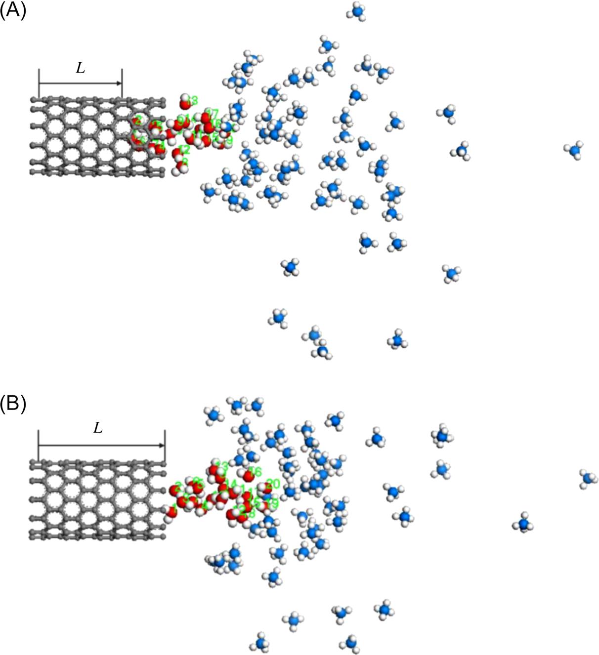
Fig. 8.7 shows overall pictures of the moving process of water molecules extracted from the SWCNTs caused by 40 methane molecules. Water molecules in the nanotube start to move to an end of the SWCNT. Simultaneously, the initial ordered configuration of methane molecules becomes disordered because of diffusion. The water molecules are drawn out to a certain distance L as shown in Fig. 8.7B. It takes 180 ps to draw all water molecules out completely from the SWCNT (as shown in Fig. 8.7C). Finally, the nanotube is empty. The methane molecules are responsible for the driving force, therefore, the effect of methane molecules on the translocation of water molecules becomes important. It is observed that the transport behavior of water molecules driven by 60 methane molecules as shown in Fig. 8.8 is much different from that driven by 40 methane molecules as shown in Fig. 8.7.

At the same simulation time 55 ps, 60 methane molecules make the water molecules move 11.798 Å shown in Fig. 8.8A while 40 methane molecules make them move 6.794 Å shown in Fig. 8.7B. The average translocation velocity is 0.2145 and 0.1235 Å/ps. Therefore, we suggest that the driving force generated by 60 methane molecules is larger than that by 40 methane molecules. An increase of methane molecules favors the reduction of the extracting time of water molecules from the CNT. As shown in Fig. 8.9, the displacement L(t) of water molecules displays roughly linear dependence on time t for different numbers of methane molecules. The translocation rate of water molecules is found to increase with the number of methane molecules. When there are 80 methane molecules, velocity can reach up to 4.817 Å/ps, almost more than 40 orders of magnitude greater than in the case of 40 methane molecules.

As for a simple SWCNT–water system, water molecules are relatively stable in the CNT. It is impossible for water molecules to escape from the interior of CNT automatically without any additional driving force. Whether the water molecules could be drawn out or not is decided by the result of competition between the methane–water attractive force and the SWCNT–water attractive force. When the methane–water attractive force is dominant and the SWCNT–water attractive force is less dominant, the water molecules could be drawn out successfully. On the contrary, when the SWCNT–water attractive force is stronger and the methane–water attractive force is weaker, the water molecules would fail to be drawn out. To ascertain this hypothesis, we perform a series of energy computations. As shown in Fig. 8.10, the difference of E2 and E1, i.e., ΔE (![]() ) is a function of the time t with different numbers of methane molecules, in which ΔE increases with time. We estimate the attractive potential energy of SWCNT–water and methane–water, defined as E1 and E2. Fig. 8.10 shows that, as time goes, methane–water attractive interaction is getting stronger than SWCNT–water attractive interaction, and methane–water attractive interaction rises as the number of the methane molecules increases. That is to say, more methane molecules would generate a stronger attractive force on the water molecules. It is the reason why more methane molecules can draw water molecules out from the SWCNTs with shorter time.
) is a function of the time t with different numbers of methane molecules, in which ΔE increases with time. We estimate the attractive potential energy of SWCNT–water and methane–water, defined as E1 and E2. Fig. 8.10 shows that, as time goes, methane–water attractive interaction is getting stronger than SWCNT–water attractive interaction, and methane–water attractive interaction rises as the number of the methane molecules increases. That is to say, more methane molecules would generate a stronger attractive force on the water molecules. It is the reason why more methane molecules can draw water molecules out from the SWCNTs with shorter time.

 ) as a function of time t with the number of methane molecules. E1 is the SWCNT–water attractive potential energy and E2 the methane–water attractive potential energy [41].
As reported [22,42], the water fluidity in CNTs increases as the diameter of the SWCNT increases. The question is how water molecules transport under an extra driving force when confined in a CNT. In Fig. 8.11, the water molecules can be easily drawn out from the (14, 0) SWCNT (diameter 10.96 Å) completely; however, it is hard to draw the water molecules out from the (16, 0) and (18, 0) SWCNTs with diameters of 12.53 and 14.09 Å in Figs. 8.12 and 8.13. This suggests that an increased diameter of the SWCNT decreases the transport velocity of water molecules. It is worth pointing out that the water molecules eventually reach up to the maximum distance in the nanotube and bounce back for some distance due to the unstable interaction force, which is the result of the competition of attractive interaction between the SWCNT–water and methane–water systems.

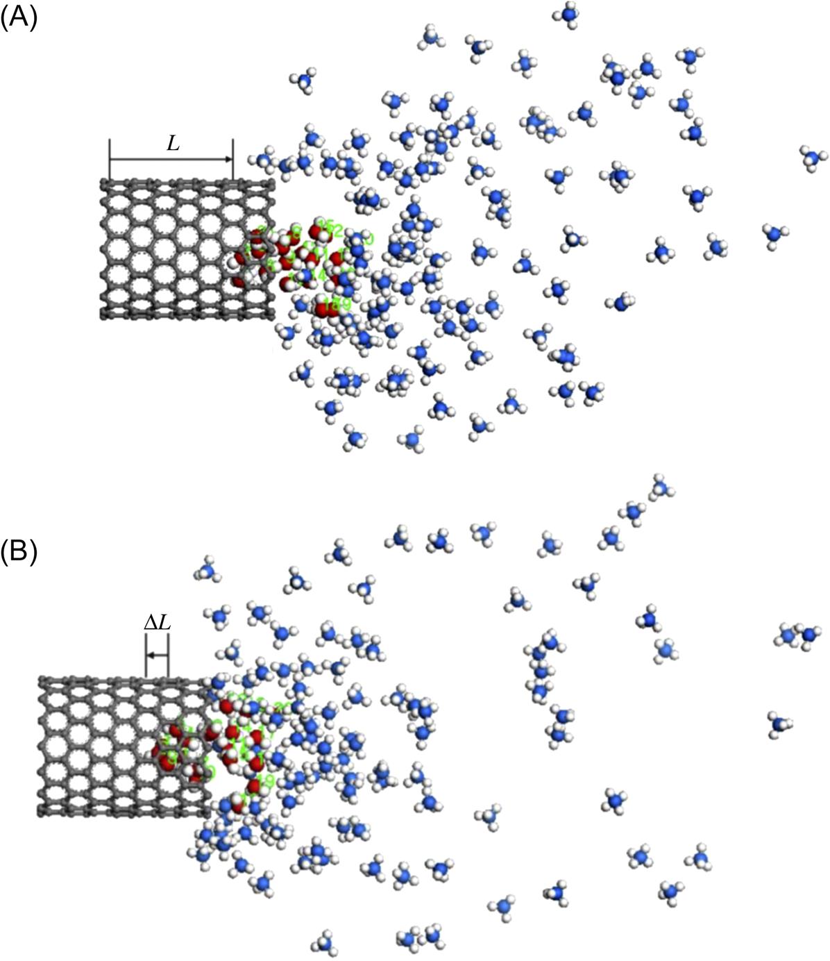
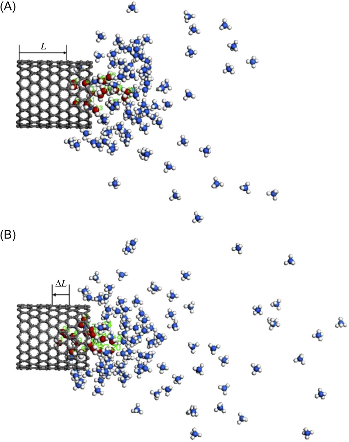
The “bounce back” distances ΔL of water molecules in Figs. 8.12 and 8.13 are 1.625 and 1.749 Å, which illustrate that the nanotube with a bigger diameter would cause a more serious “bounce back” phenomenon than that with a smaller diameter. The translocation displacement L(t) of water molecules as a function of time t with diameters of SWCNTs is illustrated in Fig. 8.14, where the curves display the opposite tendency to the Fig. 8.9.
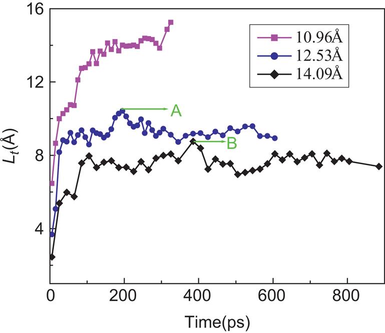
The axial translocation velocity of water molecules in SWCNT increases sharply as the diameter of the SWCNT decreases. Obviously, two curves for SWCNTs with diameters of 12.53 and 14.09 Å have their peak values, denoted by A and B. The peak value A is higher than B. They correspond to the maximum translocation distance of water molecules inside of the SWCNTs. The water molecules in the SWCNT with diameter of 12.53 Å will take less time to reach the peak value than that with diameter of 14.09 Å. Subsequently, as the maximum peak is reached, the curves begin to drop down due to the “bounce back” phenomenon illustrated in Figs. 8.12 and 8.13. The “bounce back” is due to the SWCNT–water attractive interaction being greater than the methane–water attractive interaction.
In a word, the water molecules confined in the SWCNT can be drawn out by methane molecules. The competition of attractive force between methane–water and SWCNT–water systems dominates the moving direction of water molecules. The number of methane molecules has a positive effect on the transport of water molecules through the SWCNT. The translocation velocity of water molecules increases sharply with the increasing number of methane molecules. The diameter of the SWCNT is however not in favor of the transport of water molecules. The transport velocity of water molecules decreases with the increasing diameter of the SWCNT. The “bounce back” of water molecules is clearly observed in SWCNTs as diameters get bigger.
The result may arouse interest in fabrication of molecular-selective CNT devices which may act through mechanisms similar to those of biological transmembrane channels. The filling/emptying transition in functionalized nanotubes can be potentially used as wetting–dewetting nanoscale devices and would have wide applications in nanotechnology and biotechnology.
8.2.2 Driving Water Molecules Along a Diameter-Gradient SWCNT
Water usually travels through many passages connected by junctions of different diameters, rather than single-diameter tubes, which can cause barriers to water transport. Although much work focuses on the transport of water confined in a single-diameter SWCNT [43,44], little research has been conducted on the transport behavior of water molecules in a diameter-gradient SWCNT with many junctions. The manipulation of the flow of water molecules through diameter-gradient SWCNTs connected by junctions with different diameters is a challenging issue and has not been well tackled.
MD simulation is also performed to investigate how methane molecules pull water molecules through a diameter-gradient SWCNT with junctions. The model is highly appropriate for studying the influence of junctions on the transport of water through SWCNTs with different diameters. Understanding the mechanism of water transport in these CNT-based membranes is crucial in the design of nanomachinery and synthetic membranes, and for the development of novel drug-delivery devices.
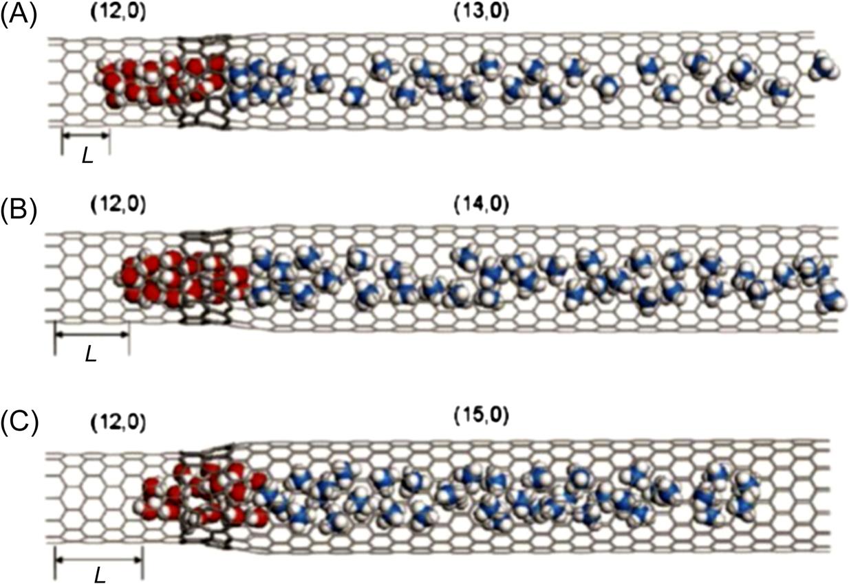
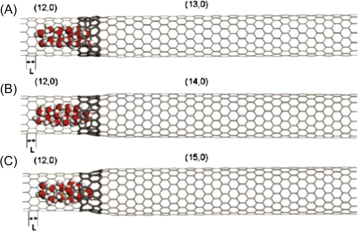
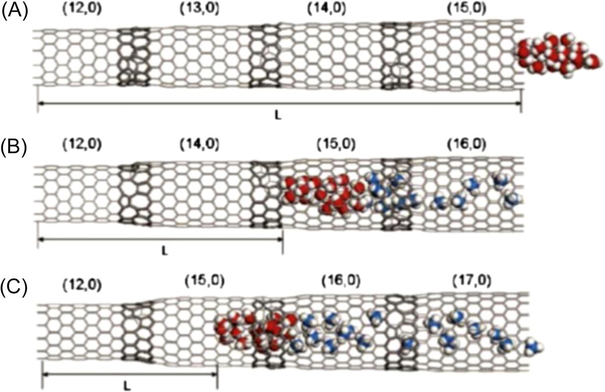
Each system consists of coaxial CNTs with different diameters, which are linked by a junction region with a pentagon–heptagon (5–7) topological structure, as illustrated in Fig. 8.15. Such connections have been directly observed by Iijima and others with transmission electron microscopy [46,47]. The nanotubes are zigzag (n, 0) SWCNTs with indices n=12, 13, 14, 15, 16, and 17, the diameters of which are 9.39, 10.18, 10.96, 11.74, 12.53, and 13.31 Å, respectively. Both bottle-like and terrace-like SWCNTs are used in the simulation. Fig. 8.15 shows the bottle-like SWCNTs, which comprise a (12, 0) SWCNT connected to (13, 0), (14, 0), and (15, 0) SWCNTs, respectively. Fig. 8.16 shows the terrace-like SWCNTs, in which (12, 0), (13, 0), (14, 0), and (15, 0) SWCNTs are connected with smooth junctions formed by five- and seven-membered rings to form a (12, 0)–(13, 0)–(14, 0)–(15, 0) series-connected SWCNT system. In the same way, other series-connected SWCNT systems are also fabricated successfully. The length of all the series-connected SWCNT systems is 83.6 Å. The coordinates of the SWCNTs are fixed. The quantity of methane molecules is chosen as 50. The cut-off distance is set to 10.0 Å, and the time-step is 1 fs. Data are recorded every 0.5 ps for further analysis. Initially, 20 water molecules are inserted randomly into the interior of the (12, 0) SWCNT, and 5000 time-steps are run to relax the initial configuration to obtain the lowest energy structure. Finally, the methane molecules are arranged in another nanotube connected with a (12, 0) SWCNT to be used to drag the water molecules from the inside of the (12, 0) SWCNT.


Fig. 8.17 shows the translocation displacement L of water molecules dragged by methane molecules through three bottle-like SWCNTs at 6000 ps. Fig. 8.17C demonstrates that the displacement distance L of water molecules in the (12, 0)–(15, 0) system is the longest and differs from the behavior of the system in the (12, 0)–(13, 0) SWCNT shown in Fig. 8.17A. Obviously, the motion of the water molecules is attributed to the methane molecules that generate the driving force to make the water molecules flow through the SWCNT. Because methane molecules confined in the SWCNT are not at the lowest energy status, they continuously diffuse with an initial acceleration. Subsequently, the water molecules will follow the methane molecules through the SWCNT due to the van der Waals attraction between the methane molecules and the water molecules. The methane molecules are responsible for the driving force, and therefore the translocation of the water molecules is dominated by the methane molecules.
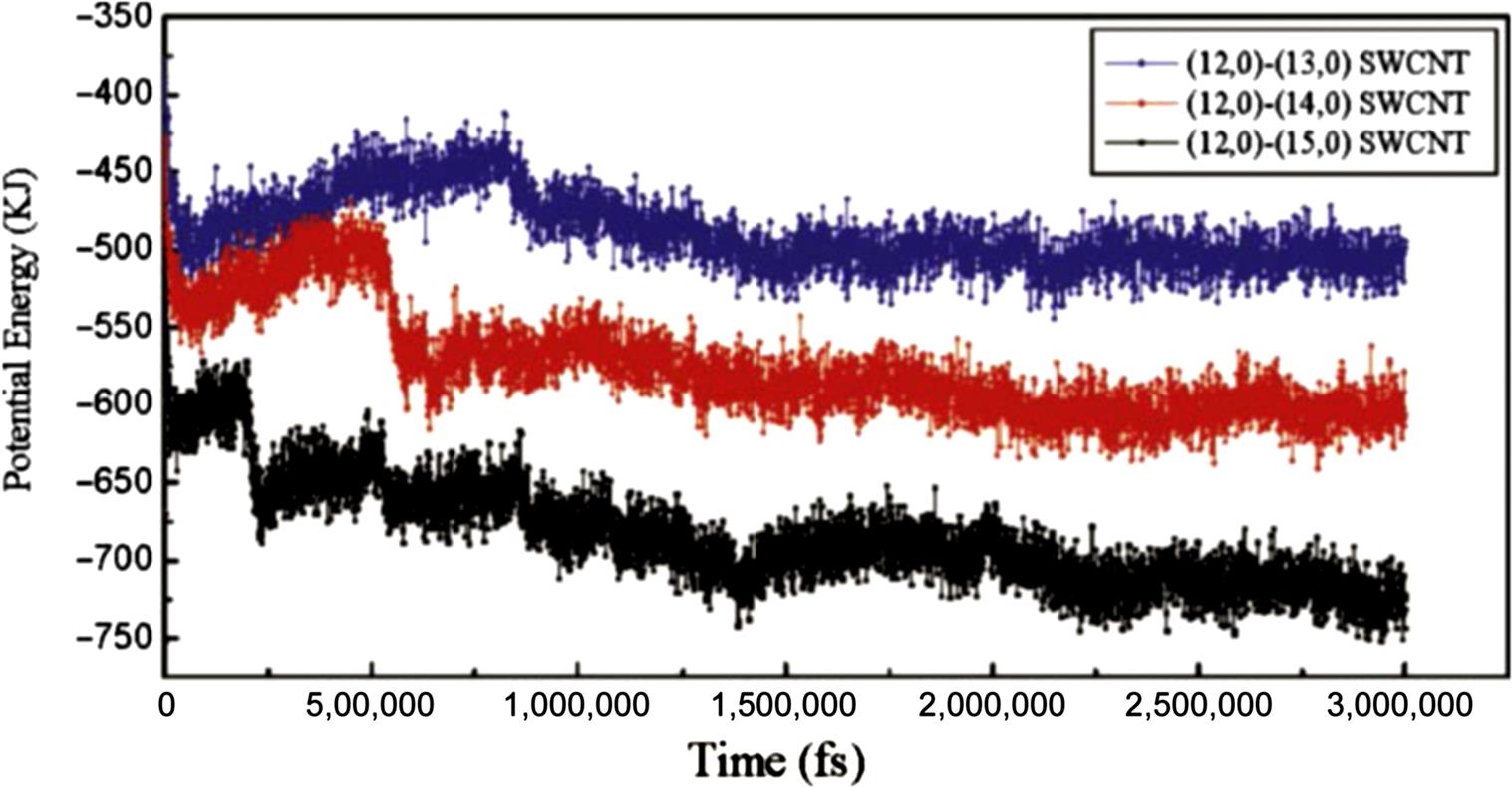
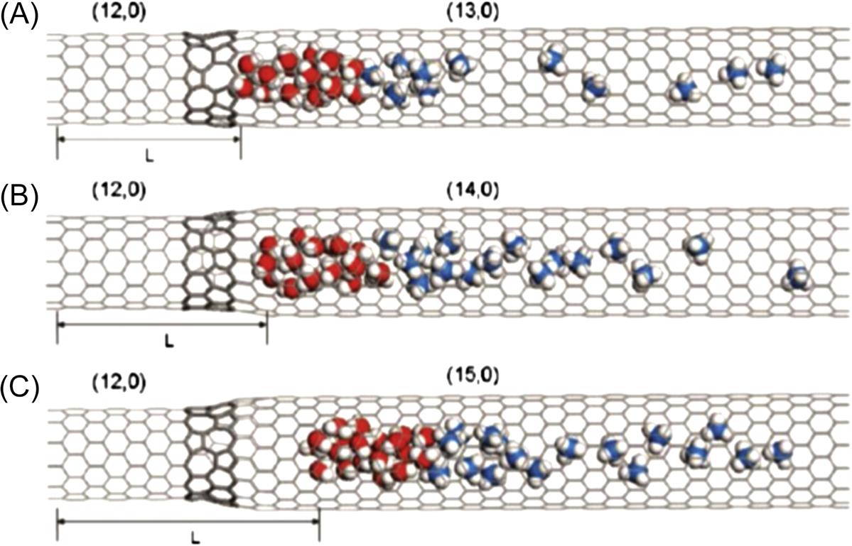
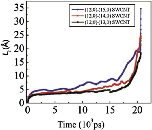
When the water molecules reach a junction region, they oscillate due to the potential barrier of the junction, which counteracts the attractive force of the methane molecules. If the attractive force of the methane molecules overcomes the potential barrier caused by the junction, then the methane molecules are able to drag the water molecules to another compartment; otherwise, they become jammed in the junction region. Fig. 8.18 shows the evolution of the potential energy in the three bottle-like systems with time. It is worthy of note that the magnitudes of the potential energy of the three systems decrease as the diameter of the SWCNTs increases. This is because the water molecules are more stable inside the bigger SWCNT than they are inside the smaller SWCNT, as demonstrated in previous work [48]. The potential energy barriers in the (12, 0)–(13, 0) SWCNT, the (12, 0)–(14, 0) SWCNT, and the (12, 0)–(15, 0) SWCNT are 75, 100, and 168 kJ, respectively, which indicates that a slight change in the diameter of a junction causes significant variation in the potential energy. In the (12, 0)–(15, 0) system, it takes the water molecules 19,330 ps to cross the junction region, whereas in the (12, 0)–(13, 0) SWCNT, it takes them about 20,550 ps to cross the junction region. The systems tend to equilibrate once the water molecules have crossed the junction region. When the methane molecules leave the interior of the SWCNTs, the attractive interaction between the methane molecules and water molecules weakens. Finally, the methane–water attractive interaction is equal to that of SWCNT–water and SWCNT–methane, which means that the whole system reaches equilibrium. Hence the number of the methane molecules in the SWCNT also affects the transport behavior of the water molecules through the nanotube. More methane molecules mean a larger driving force, and therefore it is easier for the water molecules to cross the junction region. As mentioned in Fig. 8.18, the potential energy curves display clear fluctuations around the average value, which is caused by the vibration of the water molecules in the interior of the SWCNTs at their equilibrium position in the axial direction. The final configurations of the three systems can be seen in Fig. 8.19. The maximum value of the translocation displacement of the water molecules in the (12, 0)–(13, 0), (12, 0)–(14, 0), and (12, 0)–(15, 0) SWCNTs is 18.037, 23.708, and 34.703 Å, respectively. The corresponding average velocities of the three systems are 9×10⁻⁴, 1.15×10⁻³, and 1.7×10⁻³ Å/ps. As shown in Fig. 8.20, the displacement L(t) of the water molecules displays a roughly linear dependence on time t for the different diameters of SWCNTs to which the (12, 0) SWCNT is connected. Hence, the translocation velocity of the water molecules increases with the diameter of the SWCNTs. However, for a simple SWCNT–water system without the methane molecules, as shown in Fig. 8.21, there is still a quite small displacement L of water moving toward the next compartment, which is much less than those driven by the methane molecules. Due to the interaction of the long-lasting hydrogen bonds between water molecules, it is a collective motion behavior for the confined water molecules, which is consistent with the ballistic-type mechanism of Striolo’s results [49]. When the water molecules reach a junction region, they oscillate backward and forward along the axial direction, but finally they would not spontaneously enter the next compartment due to the barrier of the junction. This is different from Hummer’s calculation in which it was found that a one-dimensionally ordered chain of water can fill a nonpolar CNT spontaneously and continuously with little resistance [19]. Likewise, our finding differs greatly from the previous investigations of fast water transport through a single-diameter CNT reported by Holt [6], Majumder [50], and Thomas [51].
To further examine the effect of a series-connected SWCNT system on the transport of water molecules, a system with more junctions, such as the terrace-like SWCNT, is designed to perform another simulation. As shown in the inset in Fig. 8.22, during the first 100 ps in the simulation, the translocation velocity of the water molecules increases with the pore size, as in Fig. 8.20. The reason is that, during the first 100 ps, the translocation displacement of water molecules in the (12, 0) (13, 0)–(14, 0)–(15, 0), (12, 0)–(14, 0)–(15, 0)–(16, 0), and (12, 0)–(15, 0)–(16, 0)–(17, 0) SWCNTs is 1.545, 1.564, and 1.573 Å, respectively, less than those in the (12, 0)–(13, 0), (12, 0)–(14, 0), and (12, 0)–(15, 0) SWCNTs (2.106, 2.360, and 2.863 Å). This indicates that the methane molecules in the terrace-like SWCNTs just start to diffuse. More junctions of the terrace-like system do not affect the diffusion of the methane molecules. The transport behavior of the water molecules in the terrace-like SWCNTs is similar to that in the bottle-like SWCNTs. Over time, an unexpected opposite trend is observed in Fig. 8.22, in that the axial translocation velocity of the water molecules in the terrace-like SWCNTs increases sharply with the decrease of the diameters of the SWCNTs connected to the (12, 0) SWCNT. This indicates that the narrower terrace-like SWCNTs give the methane molecules a greater driving force. Consequently, the translocation velocity of the water molecules increases slowly as the diameters of the SWCNTs connected to the (12, 0) SWCNT increase during the initial 100 ps but decreases rapidly with the increase in diameter after 100 ps. Fig. 8.23 shows the final snapshots of the three terrace-like systems at t) 18,000 ps. It is worth noting that the water molecules escape completely from the (12, 0)–(13, 0)–(14, 0)–(15, 0) SWCNT. The translocation displacement L (length 81.296 Å) of the water molecules is the longest in this SWCNT (as shown in Fig. 8.23A), whereas the translocation displacement L (length 35.201 Å) of the water molecules in the (12, 0)–(15, 0)–(16, 0)–(17, 0) SWCNT is the shortest (as shown in Fig. 8.23C). These results conflict with those in Fig. 8.19. Moreover, the water molecules in the terrace-like SWCNTs move further than those in the bottle-like SWCNTs over the same interval. A comparison of the results for the transport of water molecules in the bottle-like SWCNTs with those for the terrace-like SWCNTs confirms that the greater number of junctions in the terrace-like SWCNTs gives the methane molecules a more sustained driving force, which favors the rapid transport of the water molecules along the SWCNTs.

In summary, methane molecules can overcome the potential barrier caused by the junctions and successfully pull the water molecules across the junction regions from one compartment to the next. In the bottle-like SWCNTs, the junctions are detrimental obstacles to the transport of water through the nanotube, especially when the CNTs have small diameters. In contrast, for the terrace-like SWCNTs with more junctions, the junctions become a driving force that accelerates the diffusion of the methane molecules. Thus, the translocation displacement of water molecules in the terrace-like SWCNTs is much longer than that in the bottle-like SWCNTs. These results have implications for the design of nanoscale molecular diffusive drivers as motors for the transport of liquid or gas molecules. This study also indicates that the filling/emptying transition in functionalized nanotubes can potentially be used as a wetting–dewetting nanoscale device, which would have wide application in nanotechnology and biotechnology.
8.3 Hydrogen Storage [52,53]
Gas adsorption properties of CNTs [54–63] and related carbon materials, such as graphitic nanofibers [64,65], activated carbons [66–73], fullerene, and nanotanks [74–79] have been extensively studied over the last decade. However, the reported storage capacities for these materials are considerably scattered, ranging from around 2–4 wt.% [80,81] to significant 5–10 wt.% [82] values. This makes it necessary to apply theoretical quantum simulations to understand the storage mechanisms. To date, theoretical quantum calculations on the adsorption process have been carried out on many aspects, including the adsorption sites of the H2/H locating on the carbon materials [83,84], the coverage capacity of H atoms chemisorbed onto the CNTs [85,86], and the relations between hydrogen uptake capacity with the arrangements of the nanotubes [87,88], with nanotube diameter [52,85,89,90], with types of CNTs (such as zigzag, armchair, chiral, and coiled CNTs) [90–92], and with different metal doped CNTs [93–97]. Only recently has the chemisorption of hydrogen on SWCNTs been observed [98–102]. However, there is a void of information on the transient kinetics of the storage process that involves the interaction between hydrogen atoms and the CNT, and the corresponding thermodynamic properties. To obtain this important information, it is necessary to apply theoretical molecular simulation. The problem is frequently formulated in terms of potential functions, or in other words, MD or ab inito parameters. Classical potentials in MD are not always very accurate, and they usually have a simple analytical form so that numerical computations can be made faster. On the other hand, quantum mechanical ab initio methods are supposed to be highly accurate and, therefore, suitable to monitor the progress of a molecule translocating from the exterior of the CNTs into the inner space or onto the surface of the CNT tube. Although the choice of ab initio calculation methods can provide accurate results for simple molecules, the extreme computation effort makes it prohibitively difficult to produce accurate outcomes for complex molecules and macromolecules.
Additional assumptions are often required to investigate the chemical reaction process of a large cluster of molecules. Frequently applied assumptions for the H2/H chemical reaction with the graphene/CNT include treating a group of selective molecules as “fixed atoms” or simply clustering a group of molecules as environment atoms. Both methods have been utilized by many research groups. First, as regards the “fixed atoms,” it was utilized by Arellano et al. [100], who kept the CNT geometry unchanged and only varied the distances and angles of the hydrogen atoms with reference to the CNT. Verónica et al. [101] applied a similar idea by permitting the hydrogen atom to approach only from the center of the nanotube (inner wall) and imposing immobility on all the carbon atoms. Lee et al. [103] artificially set the radial component of the hydrogen atom at each step while moving the hydrogen atoms along the CNT. Although these assumptions lead to a significant reduction in computation time, it is achieved at the cost of neglecting the interactive role of the environment atoms/molecules at the vicinity of the chemical reaction sites, whose configurations often change due to the nature of the newly bonded atoms when the chemical reaction occurs.
Another method frequently observed in many reported theoretical works is the concept of a finite cluster of atoms, where atoms are cut (or taken) from the actual surface with the distance between the atoms forming the cluster kept at their bulk values [104]. This idea was applied by Han et al. [102,105], who studied the reaction pathway of hydrogen molecule reacting with CNT by applying density functional theory (DFT) calculation, with the cluster size of 100 carbon atoms. Due to the assumption of invariable carbon atoms in their work, it was not able to reflect the phenomena of C–C bond severance in the CNT sidewall caused by hydrogen interaction, which is important for the explication of CNTs coalescence observed by Nikolaev et al. [105]. One fundamental problem in the “cluster modeling” is that the convergence of the adsorption energy and the corresponding properties are associated with the cluster size. Generally, a very large cluster is required. However, if more than a few molecules are explicitly described by quantum calculation, computational costs rapidly become prohibitive.
In order to balance the efficiency and accuracy in the study of large systems, one of the popular and versatile hybrid approaches, the ONIOM (our own N-layered integrated molecular orbital and molecular mechanics (MM)), was developed by Morokuma and coworkers [106–112]. The basic concept of the ONIOM method is to divide a large system (the real system) into several layers, with each layer treated with distinct computational methods. The partition can be based on identifying the reaction center molecule. The target calculation for the relative energy is a high-level quantum mechanics (QM) treatment for the entire real system, which is usually computationally demanding and impractical. Therefore, instead of evaluating the energy of the real system at the high level, the ONIOM scheme can extrapolate it from independent less demanding calculations. The chemically important region is dealt with using the accurate high level QM method while the rest of the layers are treated with the computationally less intensive lower level QM (e.g., semiempirical) or MM methods. To date, this hybrid framework has been mostly applied to large organic molecules and organometallic complexes.
In the present work, a systematic study of the adsorption process of hydrogen atoms onto the (5, 5) CNT sidewall will be presented by taking on the two-layer ONIOM2 scheme. The corresponding thermodynamics properties are also investigated. A moderately sized active site region is described using high level theory, and the extended framework/environment atoms considered using a low-level method. With the theoretical level combination as suggested by Morokuma et al. [106–112], the integrated system energy is obtained from three independent calculations, ![]() , and
, and ![]()
where, the “real” system denotes all the complex geometry structures, which contains all the framework atoms and is calculated at the MM level. The “model” system refers to the chemical reaction sites, and its energy is treated at both the QM and MM levels, respectively. Fictitious hydrogen link atoms are used to cap those dangling bonds caused by the cutting of the covalent bonds between the QM and the MM regions. More specifically, in this study, the small model system includes the hydrogen and the necessary carbon atoms to represent the chemical activation sites, while other carbon atoms are used to simulate the local environment of the active sites during the adsorption process.
The conventional DFT calculations are directed toward obtaining electronic structure properties at absolute temperature. Therefore, in order to obtain refined and efficient simulation results at finite temperature, it is necessary to derive the corresponding thermodynamics properties from the mathematic framework that the DFT provides. The Boltzmann factor and partition functions are incorporated with DFT calculation to establish the temperature dependence of the Gibbs free energy of the electrochemical system. The transition states of the reaction are also studied in order to determine the energy barrier of the reaction and the reaction rate. It is important to note that the attractive feature of this method is that it connects seamlessly with conventional phenomenological equations for modeling macroscopic phenomena, on the basis of the intermolecular forces that the DFT uses for microscopic structure.
8.3.1 Computational Methodology and Physical Models
The model consists of a relatively narrow (5, 5) armchair CNT constituting of 180 carbon atoms with tube length of 22.6 Å, as shown in Fig. 8.24. The reason for the selection of relative smaller radii nanotubes lies in that it is much more energetically preferable than larger ones, as the C–C bonds of smaller diameter nanotubes are under greater strain [113,114]. The tube length used in this work is consistent with many earlier studies on the addition of hydrogen atoms to CNTs [84–86,115,116]. Clearly the tube caps possess higher potential energy fields and stronger attracting forces than the tube walls [86], as the electronic clouds of the carbon atoms at the caps overlap more significantly than those at the walls. In order to focus on the reaction sites at the sidewall of CNT and discount the effects caused by the tube caps, it is necessary to remove the caps during the simulation. The corresponding dangling bonds at the tube ends due to the removal are tied off with hydrogen atoms.

Our study begins with two hydrogen atoms which are physisorbed at the exterior of the CNT due to vdW attraction, see Fig. 8.25. The subsequent chemical reaction of hydrogen atoms with the sidewall of CNT, and the corresponding molecular thermodynamics properties, are then examined. In this work, the frequencies (the second derivative of energy with respect to the atomic coordinates) for the optimized intermediate and transition states are calculated to verify the correct transition structures (TSs) obtained.
The accuracy of the ONIOM scheme depends considerably on the choice of the calculation levels for the “model” and “real” regions. In this study, the small model system is treated via high-level DFT, specifically, the hybrid functional B3LYP method (Becke’s three-parameter hybrid method [117–122] with the exchange functional of Lee et al. [123]). The remaining of the framework connecting the active site is handled via the low-level universal force field (UFF) MM to reduce the computational time and to represent the proper “mechanical” confinement effect for the embedded DFT part. The UFF force field replaces the interactions of the electrons with each other and with the nuclei by explicitly approximating all these interactions with a sum of refined energy expressions. Due to the fact that the UFF force field is based on vdW parameters to approximate interatomic parameters from the atomic parameter set, it can reasonably account for vdW interactions which have been reported to have significant contributions to most absorption processes. Overall this B3LYP:UFF combination provides small geometry deviation from the target calculation, and has been suggested/recommended by several researchers [84,86,115,116].
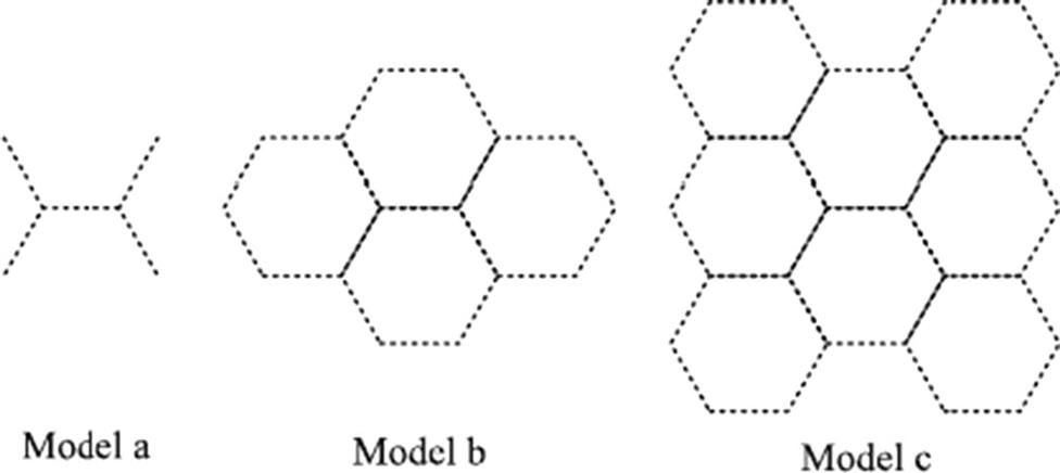
Another factor that determines the accuracy of the hybrid ONIOM method is the physical selection of the high- and low-level regions for calculation. Although the amount for each model system and the theoretical level employed for every problem varies to some extent, it is important to properly choose the region sizes for the model system. In the case of small molecules or atoms, such as the H2 or H in this work, the size for the reactant species should include those in the proximity of the surrounding atoms, which can at least interact with the reactant through vdW forces. The appropriate dimension of the “model system” is brought out more clearly by carrying out a proper convergence test for progressively different model systems. The amount of carbon atoms of the small model system was varied from 6 to 16, and then to 28, as shown in Fig. 8.25. Comparison of the adsorption energy results obtained from the 6-carbon and 16-carbon small model systems showed significant discrepancies. The subsequent comparison of the 16-carbon and 28-carbon small model systems revealed very small discrepancy of less than 0.1%, and we can, therefore, verify that the solutions have converged when using the 16-carbon small model. Thus all subsequent calculations were carried out using the 16-carbon small model.
8.3.2 Reaction Pathway of Atomic Hydrogen Interaction With CNT
The basis set of 6–31+G(d,p) is used for the small model system simulation, which emphasizes the polarization and diffusion function effects in the chemical reactions of the hydrogen atoms interacting with the CNT. The adsorption energies of the hydrogenated (5, 5) CNT systems are obtained according to Eq. (8.2). For the purpose of determining the activation barriers and understanding the chemisorptions mechanism, most of the effort here is focused on characterizing not only the stable intermediate (SI) but also the TSs states, where the latter follows the potential energy surface (PSE) path down to the SI. In principle, the transition state can be obtained from the maximum in the free energy surface projected onto the reaction coordinate, while the stable states is obtained from the minimum. In practice, there are many structural transformations (reaction pathways) that one can envision for the transformation of the same reactants into the same products. When plotting energies versus bond distances that involve bond breakage and formation to illustrate the chemical reaction process including the reactants, TS structure, intermediates, and products, the potential surfaces are often combined in three or more dimensions. In other words, the chemisorptions can proceed through a multiplicity of routes with an ensemble of TS structures. Therefore, it is more appropriate to say that we are exploring the potential energy transformation, when exploring the reaction outcome or possible mechanisms for some chemical transformations [124].
Considering the importance of SI and transition states structures in the understanding of the chemical transformation, the search, optimization and verification of the geometry for these structures were first performed with the ONIOM2 integrated schemes as part of the GAUSSIAN03 computational package. To verify the structures for the SI and TS, and to obtain the corresponding thermal properties for these structures, one more step is necessary, namely, performing the frequency analysis of the optimized structures. This vibrational frequency calculation is required to be carried out at the same B3LYP/6–31+G (d,p) level as that in the geometry optimization. From the output of these calculations, we can establish that they are true viable SI and TS structures when only one imaginary frequency (negative force constant) exists for each TS structure, while an all-positive frequency condition is required for the SI structures. The underlying theoretical basis for this is due to the TSs corresponding to the first-order saddle points on the PSE. Such a saddle point is a point where there is a minimum in all dimensions but one. The SI states are located at the minimum points on the PSE. To further verify the simulation results for the TS and SI states, the auxiliary Gauss view, which is a Graphical User Interface program, was used to visually examine structures at all steps throughout the calculations. All stable structures were verified to be geometry minima by performing quadratic potential frequency calculations and examining the frequency list for imaginary values. By computing the frequencies of the transition state structures, it was also shown that the transition states are characterized by one imaginary frequency.
Once the information on geometry optimization is obtained, it is then possible to calculate the adsorption energy for the hydrogen, which is defined according to
(8.2)
Where ECNT–2H, ECNT, and E2H are the total energies of the fully optimized CNT–2H system, the stand-alone nanotube, and the hydrogen atoms, respectively. According to this definition, the negative binding energies obtained imply that the system is stable.
To investigate the activation energy of the hydrogen chemisorptions process, we first predict the SI and TS states of the reaction. The connections between reactants, intermediates, TSs, and products are shown in Fig. 8.26, where the contour line represents the entire chemical adsorption pathway of the two hydrogen atoms being chemisorbed onto the (5, 5) CNT. The adsorption energies are calculated according to Eq. (8.2), and relative reaction energy barriers are listed in the figure as well. This figure indicates that the two hydrogen atoms first form C–H bond and eventually sever the C–C bond of the CNT to form two H–C σ-bonds, and the overall chemical transformation is an exothermal reaction. The detailed configurations at each stable and transition states can be found in Fig. 8.24, Figs. 8.27–8.29. In addition to these structures, it is interesting to examine how the geometry of the system changes along the reaction pathway. Looking at the geometrical changes, one can clearly observe the principal movements during the hydrogen chemisorption. The present calculations begin with two hydrogen atoms which are initially physisorbed at the exterior of the CNT. Following geometry optimization, they attain the SI state I (SI I) see Fig. 8.24. Experimentally, the SI I physical state can be achieved under high-pressure conditions, or by injecting hydrogen atoms with high kinetic energies into the reaction area [100]. It can be observed that, in the stable SI state structure, both of the hydrogen atoms are attracted to the exterior surface of CNT due to the vdW attraction from the exterior of the CNT, and both are directly above two carbon atoms, along the radial direction of the CNT, see Fig. 8.24. Clearly, the hydrogen atom (H1) which is nearer to the surface of the CNT weakens the C–C π-bond of the CNT, and subsequently forms the C–H σ-bond at the exterior of the CNT in SI state II (SI II), see Fig. 8.27. For convenience, we shall name the carbon atom in the C–H bond as C1. Following the reaction pathway, we found the other hydrogen atom (H2) experiences the same reaction procedure as the H1 atom. It is attracted and eventually chemisorbed with another carbon atom (C2) that is located on the same circumferential layer (of the CNT) as the first carbon atom (C1). Our results further show that the adsorption of the second hydrogen atom (H2) on the CNT wall leads to an obvious distortion of the CNT structure, the corresponding configurations are shown in Fig. 8.28. Thus, the reaction from the physisorption of the hydrogen atoms to their chemisorption has greatly changed the bonds adjacent to the reaction sites. To confirm the bond breakage, the C–C bond length change from SI I to SI III was calculated. The results show that the distance between C1 and C2 extends from 1.55 Å in SI I to 1.70 Å in SI II and subsequently to 2.49 Å in the final products of SI III, see Fig. 8.29. This distance variation clearly indicates that the C–C bond is severed when both hydrogen atoms are chemisorbed at the exterior of the CNT, in the process of attaining the most stable SI III configuration.
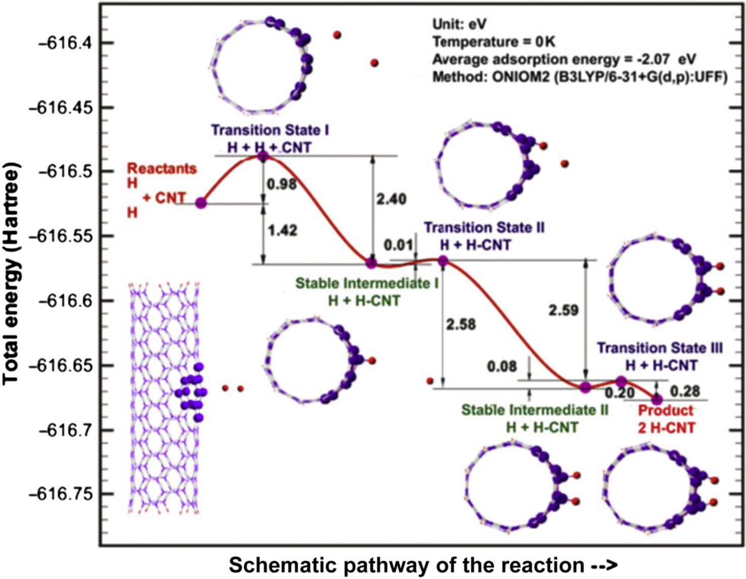

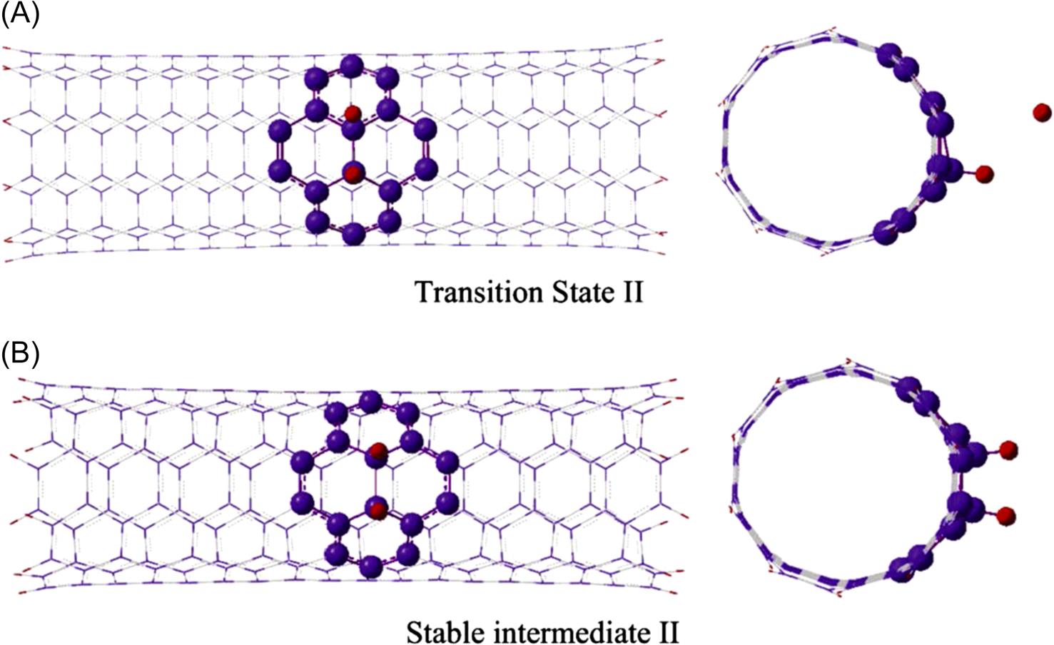
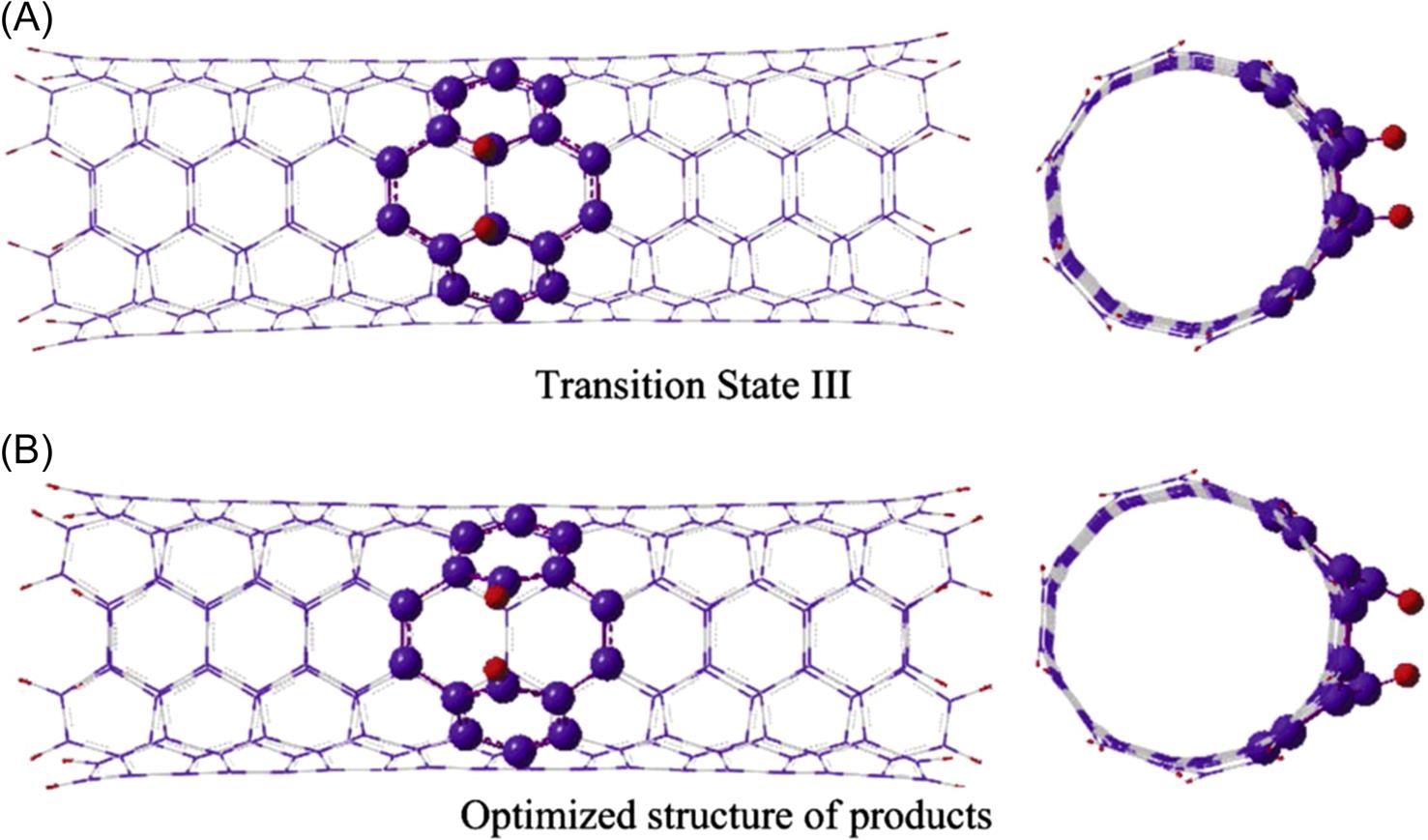
We have discussed the relative geometry variation for each state along the chemical pathway. Now we move on to examine the energy changes, which we have calculated, as the reaction progresses from each state to the next. It can be observed from Fig. 8.26 that the adsorption processes for both of the hydrogen atoms onto the sidewall of the tube are exothermic reactions. For the first hydrogen atom (H1), with the H–C bonding energy of –1.42 eV (–32.746 kcal/mol), it is evident that the reactants achieve an energetically favorable state following the chemical reaction between one hydrogen atom and the CNT. For the second hydrogen atom (H2), with –2.58 eV released from the reaction, it reaches the stable state where both H1 and H2 are chemisorbed at the exterior of the CNT, but the C–C bond remains intact, see Fig. 8.28. However, it is not the most favorable state until the C–C bond is finally severed and this severance process is still energetically favorable with –0.20 eV released. The present results of this exothermic reaction between hydrogen atoms and the CNT are different from that of the report for H2 molecules with CNT, by Han et al. [102], which indicated that the reaction is an endothermic process with 0.796 eV (18.352 kcal/mol) being absorbed by the system. The difference in the results may be due to the reason that more energy is required to break the H–H bond. To substantiate this, we note that it has been reported that about 4.565 eV (105.269 kcal/mol) will be absorbed to dissociate one hydrogen molecule into two hydrogen atoms [125].
8.3.3 Enthalpies and Free Energies of the Reaction
Thus far, for the various states of the chemisorptions process, we have obtained the energy and geometry structure of atoms and molecules from first principle calculations. However, all the above arguments are carried out at absolute temperature. A practical question thus arises as to how temperature effects will influence these stable and transition states, and how the associated molecular vibrations vary over these energy states at a given temperature.
The thermodynamic state quantities are accessible by means of mathematical relationships given by molecular thermodynamics theory [126]. The central themes to solve this problem are the Boltzmann factor Pj and the partition function Q(N, V, β). Once the ground state geometry is obtained, we are then able to extend the investigation further by studying the chemical reaction as a function of temperature T. Following the finite temperature study, the effects of Gibbs free energy, entropy, and enthalpy on the bond formation are explored in this section. Still the ONIOM scheme is applied to obtain the frequencies, while the Boltzmann factor and partition function are employed to establish the temperature dependence of the Gibbs free energy of the reaction.
In molecular thermodynamics theory, the Boltzmann factor Pj expresses the “probability” of a state at energy state Ej relative to the probability of a state of zero energy. For a system with energy states E1, E2, En, the probability of Pj in the state Ej depends exponentially on the energy of that state
(8.3)
The temperature T (in Kelvin) is introduced into the quantum level formulation by β=(kBT)−1, where kB is the Boltzmann constant. We are then able to calculate the average energy of a system in the ensemble (NVT) by
(8.4)
where Q(N, V, β) is the partition function of the system.
(8.5)
Applying the partition function, the molecular partition energy can be written as
(8.6)
The energy of a molecule E can be written as the sum of the translational, rotational, vibrational, and electronic motion energies
(8.7)
From Eqs. (8.6) and (8.7), certain thermodynamic parameters, such as the Gibbs free energy G, enthalpy H, entropy S, and the heat capacities, can be investigated. The deduction for these parameters can be found in McQuarrie [126].
To enhance our understanding of the feasibility and rates of the chemisorption process in this study, it is necessary to consider two thermodynamic properties of the reaction. These are the free energy difference, ΔG that is between the products (the final state) and reactants (the initial state), and ΔG‡ that describes the energy difference for initiating the conversion of reactants to the transition states. The former determines whether the reaction will be a spontaneous process, while the latter determines the rate of the reaction. The latter is commonly known as the Gibbs free energy of activation.
Based on the earlier results obtained in the present work, we note that it is easier for the hydrogen atom to react with the tube than the H2 molecules. The adsorption of the former is energetically favorable, suggesting that the chemisorption process occurs spontaneously. We begin with a discussion on the thermochemical properties of entropy, enthalpy, and Gibbs free energy for the reaction process from 20K to 1000K, and the results from the reactants to the final products are presented in Fig. 8.30. It is clearly observed from this figure that as temperature T increases, the enthalpy (ΔH) and entropy (ΔS) decreases, while the Gibbs free energy ΔG increases. The maximum value of the free energy is still negative, at about –33 kcal/mol at 1000K. This indicates that the chemisorption process of the hydrogen atoms onto the outside wall of the CNT is a spontaneous one, when the temperature ranges from 20K to 1000K. The negative Gibbs free energy (ΔG) also indicates an exergonic process, where the system releases energy to its surroundings during the chemisorption process. Throughout the chemical transformation, the reactants change into the products, release the stored energy, and gradually the system reaches a stable condition of equilibrium. The magnitude of the free energy change is a measure of the “driving force” behind the reaction. The larger this magnitude is, which in this case occurs at lower temperatures, indicates that the reaction process is more likely to take place. Thus, the reaction with ΔG=−95 kcal/mol at 20K has a higher probability of occurring than that of ΔG=−33 kcal/mol at 1000K, see Fig. 8.30. The magnitudes of the enthalpy and entropy are decreasing as well, and the spontaneous change in these properties is often referred to as structural relaxation.

The next issue that naturally arises is whether we can explain the reaction rate in terms of the thermos dynamic properties. The free energy difference between reactants and products accounts for the equilibrium of the reaction, and a negative ΔG only provides information that a reaction can occur spontaneously, but it does not reveal whether it will proceed at a perceptible rate. In other words, the reaction speed is largely unrelated to the ΔG of the reaction. To determine how quickly the equilibrium state is attained, the Gibbs free energy of activation (ΔG‡) which regulates the rate of the reaction has to be considered. The free energy of activation ΔG‡ is sometimes simply called the activation energy, which can be obtained from the difference of the free energy between the transition-state intermediate and the reactant. As ΔG‡ generally has a very large positive value, only a small fraction of the reactant molecules will at any one time acquire this free energy, and the overall rate of the reaction will be limited by the rate of formation of the TS. Thus, we have to consider not only the end points of the reaction, but also the chemical pathway between the end points.
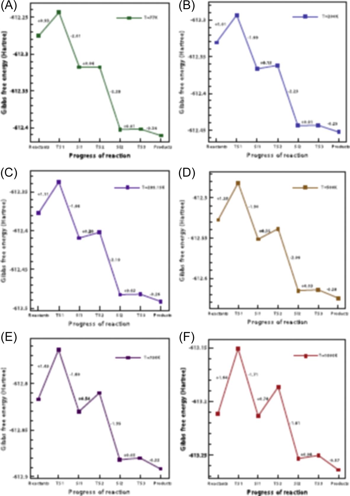
Fig. 8.31 shows the variation of ΔG‡ at typical temperatures, and the corresponding activation energies are illustrated in the plots of Fig. 8.32 which chart the changes in ΔG. These curves reveal that the reaction is more accelerated at lower temperatures due to the resulting lower activation energy between the reactants and its transition state intermediate. To summarise, a pristine CNT can interact with hydrogen atoms at ambient temperatures since the reaction for the chemisorption occurs spontaneously, but to improve (increase) the reaction rate, the reaction temperature should preferably be lower since the activation energy is found to be smaller at lower temperatures. This can be clearly seen in Fig. 8.32, where at 77K the activation energies from the reactants and SI states to the respective subsequent TS states are lower than at other higher temperatures.

We reach a similar conclusion for the reaction rates. The rate coefficient for the overall reaction rate can be calculated according to the Arrhenius equation
(8.8)
where c° represents the concentration constants. Eq. (8.8) provides an illustration of the physical time-scales involved. Comparing the reaction rates at 77K and 1000K for overcoming the energy of activation from the reactants to the first SI state, we have k(77K):k(1000K)=1:133. It shows that an increase of 0.71 eV in ΔG‡ leads to a 133-fold decrease in the reaction rate. Thus relatively small changes in ΔG‡ can lead to large changes in the overall rate of the reaction. Again, we can see that the reaction at higher temperatures is indeed slower, as one would now come to expect.
8.4 Mass Detection
Nanomechanical resonators provide methods for highly sensitive mass detection of virus, gas, and other molecules. Generally, the sensitivity depends on how the resonance frequency or surface stress of a resonator changes when additional mass is adsorbed onto its surface [127–129]. Carbon nanostructures supposedly have the potential for ultra sensitive mass detection due to their extremely small size with combined extraordinary stiffness and low mass density. The vibration characteristics of carbon nanostructures have been studied in much experimental [130–133] and theoretical research [127,134–141]. With fundamental frequencies of the order of terahertz [134,140], cantilevered or bridged SWCNTs may have a mass sensitivity of up to 10−21 g when used for mass detection [127]. Is there any method which leads to more sensitive mass detection? The answer is Yes. Here we suggest a new strategy for ultra sensitive mass detection via SWCNC resonators. Since the experimental discovery in 1994 [142], CNCs with all five apex angles have been synthesized [143]. Recently, CNCs have also attracted much attention due to their unusual form. To the best of the knowledge of the authors, although a few publications have reported vibration characteristics of CNCs [144,145], studies focusing on mass sensitivity of CNC resonators are still inadequate. Hu et al. [144] simulated free transverse vibrations of open-ended single-wall CNCs (SWCNCs) using MD and Timoshenko beam model, and compared fundamental frequencies of SWCNCs with those of equivalent SWCNTs. Their MD results reveal that fundamental frequencies of SWCNCs with an apex angle of 19.2 degrees and a top radius of 0.34 nm are several times larger than those of equivalent SWCNTs. A higher resonant frequency implies a higher mass sensitivity. Besides, another natural characteristic of CNCs, its damping or quality factor, determines the energy storage time, which also plays an important role in mass detection. It should not be neglected that the quality factor decreases significantly due to surface effects as the mechanical resonator scales down. Jiang et al. [146] theoretically predicted that the favorable properties for CNTs include a high Young’s modulus and low density, giving rise to a ultrahigh quality factor with the order of 2×10⁵ via classical MD. Later, Hüttel et al. [147] experimentally measured the quality factors for CNTs and they observed gate-tunable resonances with resonance frequencies of approximately 350 MHz and quality factors of over 105. Such a large quality factor makes CNTs extremely suitable for mass detection. CNCs and CNTs are both carbon based nanomaterials with the same crystal lattice microstructures and thus have similar natural characteristics. For example, it is found that SWCNCs have high Young’s moduli of the same order as the equivalent SWCNTs [148,149]. Therefore, it is reasonable to suggest that CNCs possess similar high quality factors as CNTs. The above studies clearly confirm the suitability of using carbon nanocones for the ultra sensitive mass detection.
So far, there are no studies of mass sensitivity of SWCNC-based mass detectors. The target of this study is to explore frequency shifts of cantilevered SWCNC resonators when extra mass attached at the free end using higher-order gradient theory. Various cantilevered SWCNC and SWCNT resonators with different top radii and lengths are simulated to exhibit the outstanding performance of SWCNC resonators in mass detection.
A SWCNC is treated as being formed by rolling up a fan-shape graphite sheet and connecting its two sides together into a seamless hollow conical structure. In the hexagonal crystal lattice microstructure, each atom connects it to three neighboring atoms by covalent bonds and we adopt this as a representative cell. The unique conical structure leads to a monotonically increasing radius along the longitudinal direction which gives rise to a change in the deformation at different positions. In addition, each atom in the SWCNC possesses a different chirality even at the same level [148,150].
The deformation process of an initial equilibrium SWCNC mapped from an initial equilibrium graphite sheet is divided into two steps. Firstly, the SWCNC is just rolled rigorously from the initial equilibrium fan-shaped graphite sheet which can be precisely described by geometrical conditions:
(8.9)
 (8.9)
(8.9)
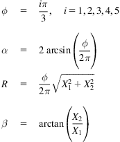
where ![]() is nodal coordinate of the formed SWCNC,
is nodal coordinate of the formed SWCNC, ![]() is the angle of the graphite sector,
is the angle of the graphite sector, ![]() is the apex angle of the cone, and R is the radius of the corresponding section. These parameters are determined by:
is the apex angle of the cone, and R is the radius of the corresponding section. These parameters are determined by:
(8.10)
 (8.10)
![]() and
and ![]() are the first- and second-order deformation gradients tensors in the rolled process. The achievement of the minimum-potential configuration of a SWCNC in the second step will be introduced as follows.
are the first- and second-order deformation gradients tensors in the rolled process. The achievement of the minimum-potential configuration of a SWCNC in the second step will be introduced as follows.
8.4.1 The Initial Equilibrium SWCNC
In the investigation of resonant frequency shifts of SWCNCs when attached to extra mass, the initial equilibrium configuration with the consideration of edge effect is obtained by the following two steps. The deformation of a SWCNC is first mapped rigidly from the initial equilibrium graphite sheet and then follows an optimized process of minimizing the potential of the system to obtain the initial equilibrium SWCNC. Therefore, the first- and second-order deformation gradients are calculated by the following two terms:
(8.11)
where ![]() and
and ![]() denote the gradients arrived from the process of rolling rigidly the planar graphite sheet to a SWCNC in the first step.
denote the gradients arrived from the process of rolling rigidly the planar graphite sheet to a SWCNC in the first step. ![]() and
and ![]() in the second step are approximated by MK interpolation:
in the second step are approximated by MK interpolation:
(8.12)
where n is the total number of nodes covered in the compact support domain. The MK interpolation is built in the two-dimensional sheet and the quadratic basis is adopted.
Consequently, we obtain the incremental equation of the system:
(8.13)
The initial equilibrium configuration of the SWCNC with the consideration of edge effect is achieved by iteratively solving the incremental equation until the nonequilibrium force (the right of Eq. (8.13)) reaches zero. Similarly, the initial equilibrium configuration of the SWCNT with the consideration of edge effect can be obtained using the above approach.
8.4.2 Analysis of Resonant Frequency and Frequency Shift
Hamilton’s principle is employed to study the resonant frequency and frequency shift of cantilevered carbon nanostructure-based mass detectors. The real solution of history of motion during period t1~t2 is determined by minimizing the Lagrangian functional:
(8.14)
where E(t) and W(t) denote kinetic energy and elastic energy stored in carbon nanostructures, and L(t) is total work done by the external force on the body and is not considered due to being free of external force. Variations of kinetic energy of the system and elastic energy stored in nanostructures are:
(8.15)
(8.16)
where ![]() is the area mass density calculated by
is the area mass density calculated by ![]() with mc being 1.9943×10⁻²³ g.
with mc being 1.9943×10⁻²³ g.
Substituting Eqs. (8.16) and (8.15) into Eq. (8.14), we can derived the dynamic equation of the system as follows:
(8.17)
Considering the field function ![]() , Eq. (8.17) can be rewritten as:
, Eq. (8.17) can be rewritten as:
(8.18)
where ![]() is angular frequency. For simplification, we denote
is angular frequency. For simplification, we denote ![]() , and
, and ![]() . Solutions of resonant frequencies become a matter of solving eigenvalue problems. The resonant frequency is sensitive to the resonator mass matrix MA and thus a change in extra mass attached at the free end of cantilevered carbon nanostructure resonator results in a variation in resonant frequency. The critical issue of mass detection is the magnitude of frequency shift corresponding to the attached mass. A larger frequency shift of resonators with the same added mass implies greater sensitivity for mass detection. That is to say, the mass sensitivity is determined by the magnitude of resonant frequency shift.
. Solutions of resonant frequencies become a matter of solving eigenvalue problems. The resonant frequency is sensitive to the resonator mass matrix MA and thus a change in extra mass attached at the free end of cantilevered carbon nanostructure resonator results in a variation in resonant frequency. The critical issue of mass detection is the magnitude of frequency shift corresponding to the attached mass. A larger frequency shift of resonators with the same added mass implies greater sensitivity for mass detection. That is to say, the mass sensitivity is determined by the magnitude of resonant frequency shift.
The higher-order gradient theory is adopted to calculate the resonant frequency and frequency shift of cantilevered SWCNC resonators, according to the attached mass at the free end. This theory can give a good prediction of fundamental frequencies of carbon nanostructures. To illustrate this point clearly, we select cantilevered 19.2 degrees SWCNC and SWCNT as examples. The initial equilibrium SWCNC has a height of 4.33 nm and a top radius of 0.34 nm. The fundamental frequency of this cantilevered SWCNC obtained using the present method is 0.393 THz, which is quite close to that of Hu et al.’s result obtained using molecular dynamic simulation (approximately 0.4 THz) [144]. In addition, the obtained fundamental frequency of a cantilevered 6 nm long (7, 7) SWCNT using the present method and atomistic simulation are, respectively, 9.006×10⁻² THz and 8.989×10⁻² THz, with only an 0.19% difference. Therefore, the above comparative studies confirm the accuracy of the present approach.
To investigate the mass sensitivity, numerical simulation of kinds of SWCNC-based mass detectors with apex angles of 19.2 and 38.9 degrees is carried out, along with the equivalent SWCNT-based mass detectors. Fig. 8.33 depicts the schematic of cantilevered SWCNC- (A) and SWCNT-based mass detectors (B) with attached mass at the free end.

Fig. 8.34 demonstrates fundamental frequencies of cantilevered SWCNCs and (7, 7) SWCNT resonators with the same top radius of 0.48 nm. It clearly reveals that the two kinds of SWCNCs with apex angles of 19.2 and 38.9 degrees exhibit far higher fundamental frequencies than equivalent SWCNTs. To further illustrate this feature, we select the cantilevered 19.2 degrees SWCNC and SWCNT resonators with the same length of 6 nm as an example. The fundamental frequency of 19.2 degrees SWCNC resonator is 0.282 THz, while that of the SWCNT resonator is only 0.090 THz, indicating a greater potential of SWCNC resonators to be used for high-performance mass detection than SWCNT resonators. The curves of these two kinds of cantilevered SWCNC resonators demonstrate that the apex angle has a slight decreasing effect on fundamental frequencies. It is worthwhile to note that the heights of these two kinds of nanostructures distinctively affect fundamental frequencies. Fundamental frequencies decrease sharply as heights of SWCNCs increase. A decline of 51.75% is observed in the fundamental frequency of 19.2 degrees SWCNC resonator as the height increases by twofold. This suggests that reduction of the size of resonators can markedly enhance the mass detection ability.
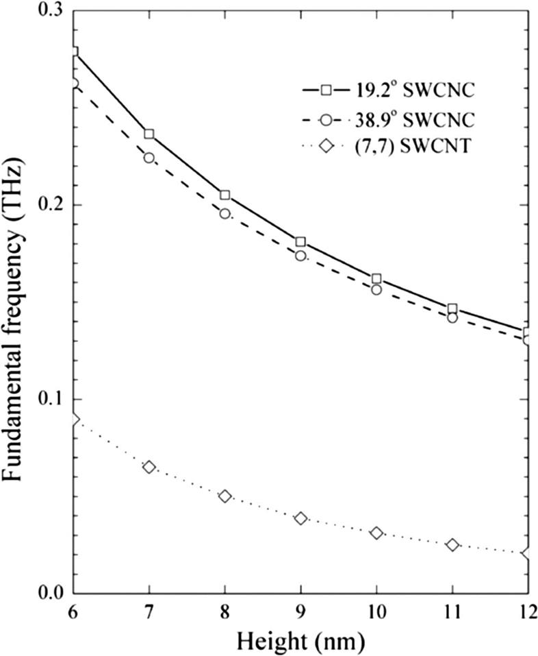
Fig. 8.35A demonstrates resonant frequencies of cantilevered (7, 7) SWCNT resonators with attached mass at the free end. The frequency-attached mass curves of SWCNT resonators show a clear variation of resonant frequency when the attached mass is larger than 10−21 g, implying the mass sensitivity of SWCNT resonators can reach a level of 10−21 g. This conclusion is in agreement with the conclusion of Li and Chou using the molecular structural mechanics method [127]. Frequency shifts of cantilevered SWCNT resonators by attached mass are shown in Fig. 8.35B. Apparently, the shortest SWCNT resonator has an evident change of frequency shift especially when the attached mass changes from 10−20 to 10−21 g. This confirms the aforementioned suggestion that reducing the size of resonators provides a way of improving the mass detection ability.

Logarithmically linear functional relationships exist between resonant frequencies of cantilevered SWCNT resonators and the attached mass if the attached mass is larger than 10−20 g. This conclusion is also applicable to the cantilevered SWCNC resonators. Fig. 8.36A shows the comparison of resonant frequencies of cantilevered SWCNC and (7, 7) SWCNT resonators with the same height of 6 nm and top radius of 0.48 nm by attached different mass. It reveals that the resonant frequency of cantilevered 38.9 degrees SWCNC resonator has a parallel trend as that of the (7, 7) SWCNT resonator and much higher than the 19.2 degrees SWCNC resonator in most cases although it possesses a lower fundamental frequency. In other word, the cantilevered 38.9 degrees SWCNC resonator is not as sensitive as the 19.2 degrees SWCNC resonator when attached to the same extra mass at the free end. It is noteworthy that the same conclusion can be even extended to 19.2 degrees SWCNC resonators if the attached mass is larger than 10−21 g which is a magnitude more sensitive than other two resonators. On the other hand, curves shown in Fig. 8.36B display clearly that both two kinds of cantilevered SWCNC-based mass detector exhibit much higher frequency shifts than cantilevered SWCNT-based ones when attached a extra mass smaller than 10−20 g. Nevertheless, the changes in frequency shifts of cantilevered 19.2 degrees SWCNC-based mass detector are far larger than SWCNT-based ones and also the 38.9 degrees SWCNC-based mass detectors when the attached mass is smaller than 10−20 g. The frequency shift of a cantilevered 19.2 degrees SWCNC-based mass detector with an attached mass of 10−21 g is 74.1464 GHz, while that of the 38.9 degrees SWCNC- and the equivalent SWCNT-based mass detector are only 22.022 and 11.096 GHz, respectively. A larger resonant frequency shift is much easier to be detected, which means 19.2 degrees SWCNC resonators are most sensitive than the others. When the attached mass changes from 10−20 to 10−21 g and from 10−21 to 10−22 g, the changes of frequency shifts of the 19.2 degrees SWCNC-based mass detector are 132.256 and 71.220 GHz, respectively; while the changes in 38.9 degrees SWCNC- and SWCNT-based mass detectors are, 105.673 and 19.838 GHz, 35.078 and 9.807 GHz, respectively, for the same changes in attached mass. Therefore, we can concluded that the mass sensitivity of the cantilevered 19.2 degrees SWCNC-based mass detector can reach a level of 10−22 g from the comparison of the changes in the frequency shifts when the attached mass changes from 10−21 to 10−22 g.
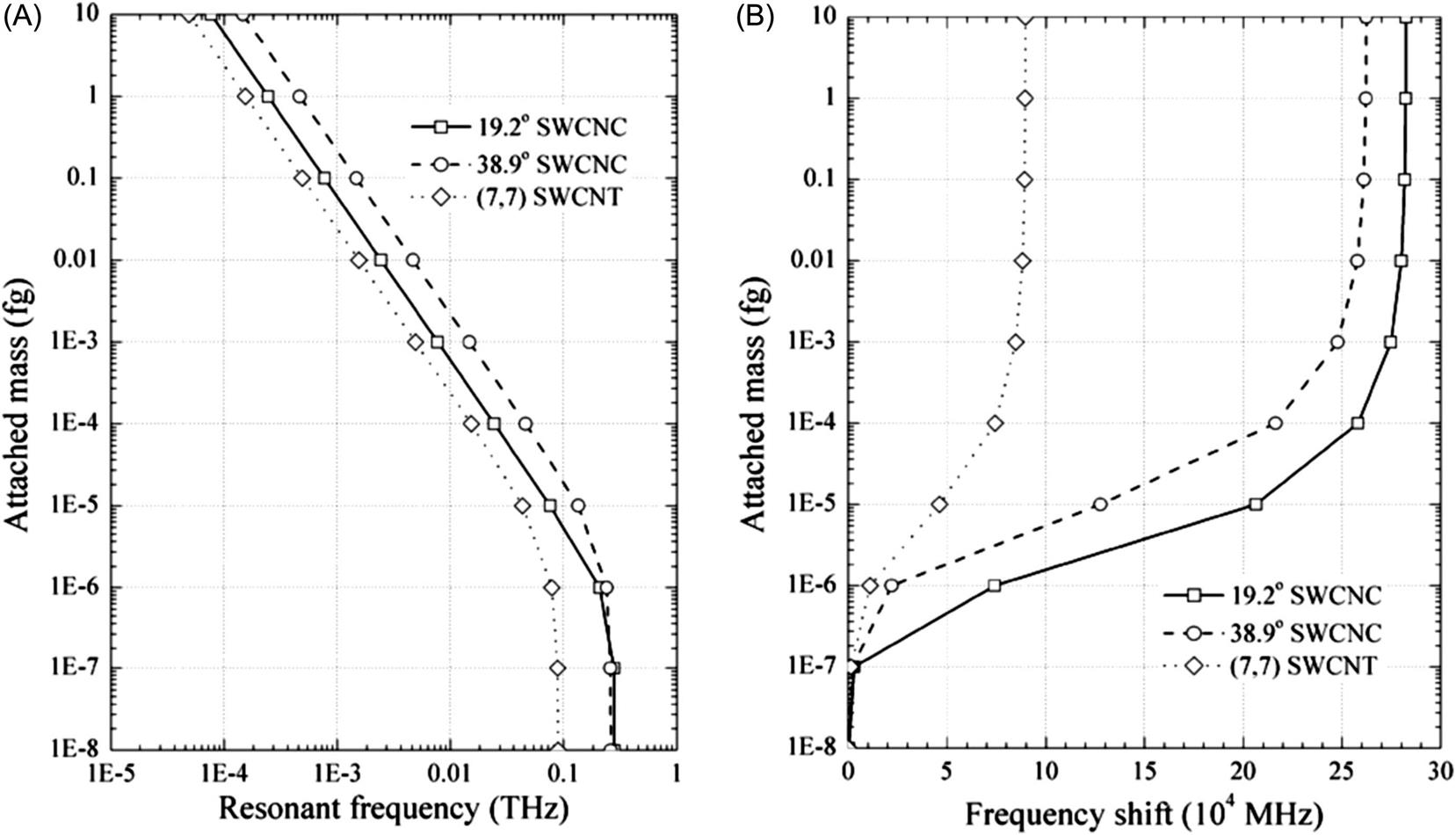
Figs. 8.37–8.40 present the resonant frequency and frequency shift of cantilevered SWCNC-based mass detectors with different apex angles, top radii, and heights obtained using the present method. Fig. 8.37 shows the resonant frequency and frequency shift of the cantilevered 19.2 degrees SWCNC-based mass detector with top radius of 0.48 nm and different height by attached extra mass at the free end. An interesting phenomenon shown in Fig. 8.37A is that the height of SWCNC resonators plays an insignificant role on the resonant frequency when the attached mass is larger than 10−20 g. Correspondingly, Fig. 8.37B shown the three curves are quite parallel to each other when the attached mass is larger than 10−20 g. It reveals that the changes of frequency shift of the three kinds of 19.2 degrees SWCNC-based mass detectors, owing to the variation of attached mass, are the same. This special characteristic offers better practicability in practical application because the fabrication process of a 19.2 degrees SWCNC-based mass detector is not as demanding as a SWCNT-based mass detector. A deviation in the size of SWCNC resonators causes a slight loss of accuracy of precision.
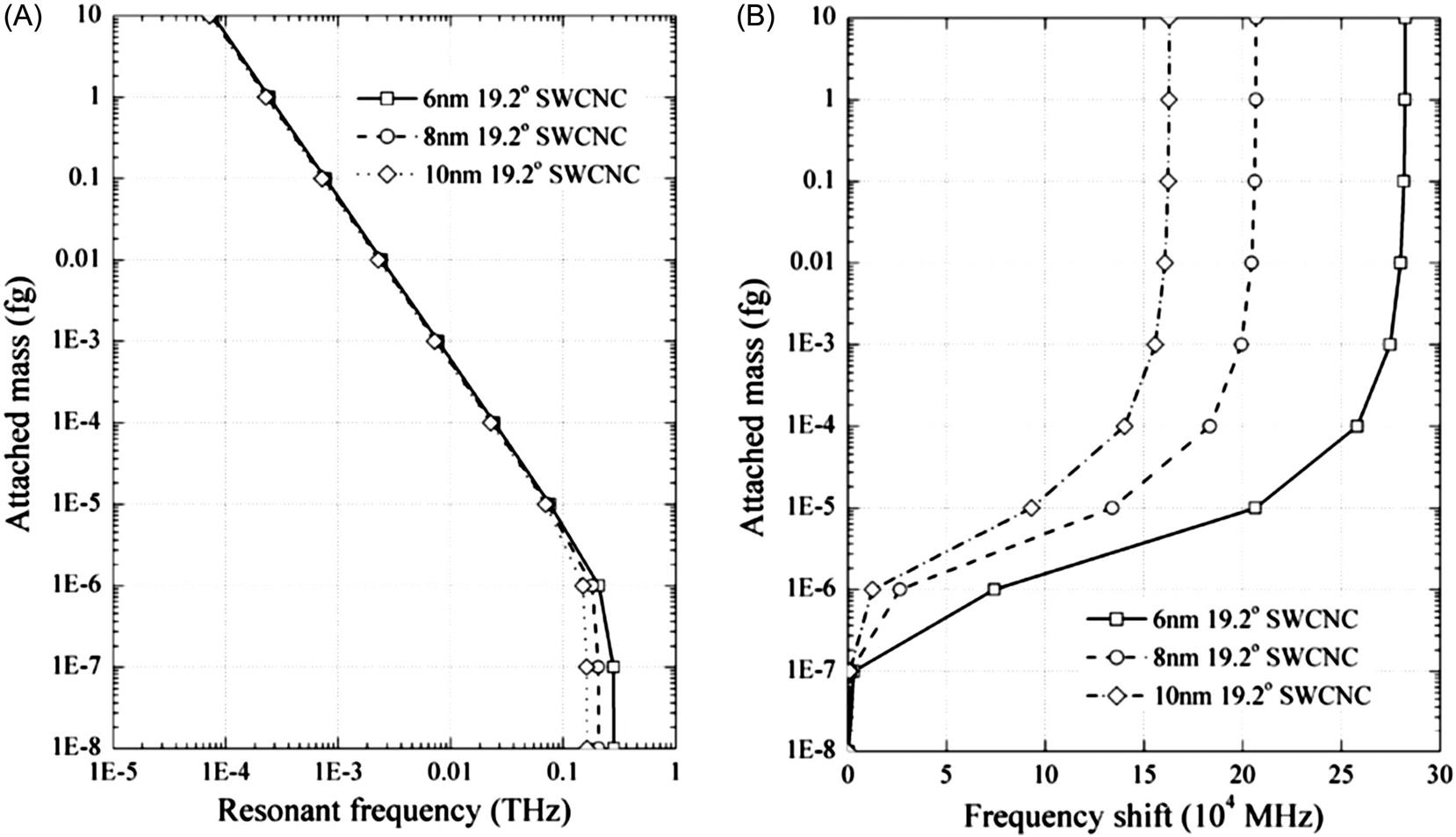

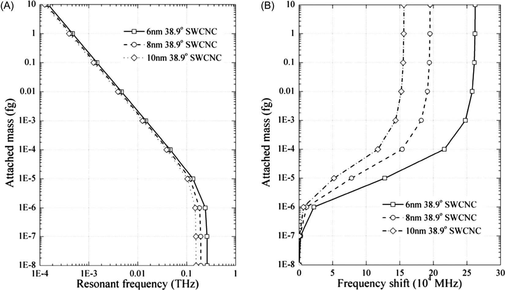

The resonant frequency and frequency shift of cantilevered 19.2 degrees SWCNC-based mass detectors with a top radius of 0.34 nm and different heights shown in Fig. 8.38A demonstrates that as the top radius of SWCNC resonator decreasing, the difference of resonant frequency between SWCNC resonators with different height becomes larger.
Figs. 8.39 and 8.40 indicate that as the apex angle increases, the cantilevered SWCNC-based mass detectors become similar to the equivalent SWCNT-based mass detector. The apex angle has a decreasing effect on the mass sensitivity of a SWCNC-based mass detector.
The effect of top radii of SWCNCs on frequency shifts is also examined. The two kinds of SWCNC resonators with different top radii and apex angles are simulated and computational results are showed in Figs. 8.41 and 8.42. The change of the top radius gives rise to a slight deviation of the frequency shift-attached mass curve and as the apex angle increases, the change becomes even smaller. It indicates that the frequency shift is slightly dependent on the top radius of SWCNC-based mass detectors.


We further investigated the high-performance of SWCNC resonators and SWCNT resonators in mass detection, numerical simulations of extra masses attached at arbitrary places. The axial distance between the attached place and free end is denoted as d. Here we introduce a geometrical parameter ![]() which is defined as
which is defined as ![]() , where L is the total length of mechanical resonators and the lengths of samples are selected as 6 nm. Figs. 8.43 and 8.44 show the variations of resonant frequency shift for cantilevered SWCNTs and SWCNCs with extra masses of 10−22 and 10−21 g versus different attached positions on the surface. Keeping the mass constant, it is observed that the frequency shifts for both SWCNC and SWCNT resonators decrease sharply as
, where L is the total length of mechanical resonators and the lengths of samples are selected as 6 nm. Figs. 8.43 and 8.44 show the variations of resonant frequency shift for cantilevered SWCNTs and SWCNCs with extra masses of 10−22 and 10−21 g versus different attached positions on the surface. Keeping the mass constant, it is observed that the frequency shifts for both SWCNC and SWCNT resonators decrease sharply as ![]() increases. With an extra mass of 10−22 g, the frequency shift for the 19.2 degrees SWCNC resonator decreases more than two times and sixteen times when the extra mass moved from the free end to the positions
increases. With an extra mass of 10−22 g, the frequency shift for the 19.2 degrees SWCNC resonator decreases more than two times and sixteen times when the extra mass moved from the free end to the positions ![]() and
and ![]() . This indicates that the sensitivity is largely dependent on the position of the mass. The free end is the most sensitive position. The 19.2 degrees SWCNC resonator has the highest sensitivity. Keeping the same top radius, when the geometrical parameter
. This indicates that the sensitivity is largely dependent on the position of the mass. The free end is the most sensitive position. The 19.2 degrees SWCNC resonator has the highest sensitivity. Keeping the same top radius, when the geometrical parameter ![]() is larger than 0.6, only a small discrepancy in frequency shift for 38.9 degrees SWCNC and (7, 7) SWCNT is observed.
is larger than 0.6, only a small discrepancy in frequency shift for 38.9 degrees SWCNC and (7, 7) SWCNT is observed.


In a word, the potential of cantilevered SWCNC resonators for use in mass detection was examined using the higher-order gradient theory under a mesh-free computational framework based on MK interpolation. Since resonant frequencies of SWCNC resonators are several times higher than those of equivalent SWCNT resonators, SWCNC resonators are more promising for application in mass detection. The shifts of resonant frequencies of SWCNC-based mass detectors are far larger than those of SWCNT-based mass detectors when the same mass is attached at the free end, implying the former has a sensitivity higher than the latter. Comparison of shifts of frequencies of carbon nanostructure-based mass detectors shows that mass sensitivity of 19.2 degrees SWCNC-based mass detectors can at least reach a level of 10−22 g. The examination of the effect of top radii on frequency shifts demonstrates that mass sensitivity of SWCNC-based mass detectors is slightly dependent on top radii and decreases as the apex angle increases.