
where ![]() is the radius of a basic circular support. The radius
is the radius of a basic circular support. The radius ![]() is determined by searching for sufficient adjacent nodes to satisfy the basis. For example, we can designate the support to cover just the three nearest neighboring nodes.
is determined by searching for sufficient adjacent nodes to satisfy the basis. For example, we can designate the support to cover just the three nearest neighboring nodes.
The size of a rectangular support can be defined by
(4.87)
where ![]() defines a basic support that is determined by searching for sufficient neighboring nodes to satisfy the basis in both directions. For the regular collocation of nodes,
defines a basic support that is determined by searching for sufficient neighboring nodes to satisfy the basis in both directions. For the regular collocation of nodes, ![]() and
and ![]() can be determined by the distance to the nearest neighboring nodes in two directions.
can be determined by the distance to the nearest neighboring nodes in two directions.
The size of the compact support (or DOI) determines the number of nodes N in the construction of matrix ![]() . The number of nodes N should be large enough to ensure that
. The number of nodes N should be large enough to ensure that ![]() is invertible. The size of each node’s DOI can be different, and it depends on the spacing density of the nodes in the local context. Small support sizes may affect the convergence of the mesh-free solutions. Large support sizes ensure convergence, but increase the computational time. Furthermore, if the support of a node extends far outside the boundary of the problem domain, then the computation size of the domain that is decided by all of the supports will be very different from the actual, which will inevitably affect the computational results. Therefore, for a given
is invertible. The size of each node’s DOI can be different, and it depends on the spacing density of the nodes in the local context. Small support sizes may affect the convergence of the mesh-free solutions. Large support sizes ensure convergence, but increase the computational time. Furthermore, if the support of a node extends far outside the boundary of the problem domain, then the computation size of the domain that is decided by all of the supports will be very different from the actual, which will inevitably affect the computational results. Therefore, for a given ![]() , increasing the number of nodes will decrease the support size and make the computational size of the domain coincide with its actual size. According to the literature,
, increasing the number of nodes will decrease the support size and make the computational size of the domain coincide with its actual size. According to the literature, ![]() is typically in the range of 2.0–4.0.
is typically in the range of 2.0–4.0.
In the later numerical simulations, the mesh-free nodes are uniformly collocated along the axial and circumferential directions (see Fig. 4.15). Two simple examples are tested to discuss the choice of the parameter ![]() for the present problems.
for the present problems.
4.5.4 MK Interpolation
Kriging can be traced to the first application in geostatistics [123] for spatial interpolation and was used for construction of the shape function and its derivatives. Similar to the MLS approximation, Kriging interpolation can also be extended to any subdomain ![]() —termed MK interpolation. We consider a distribution function
—termed MK interpolation. We consider a distribution function ![]() in a subdomain
in a subdomain ![]() . The subdomain is represented by a series of dispersive nodes xi (i=1, 2, …, n), where n is the total number of nodes covered in the subdomain. With n given field values u(x1), u(x2), … u(xn), the approximate field function
. The subdomain is represented by a series of dispersive nodes xi (i=1, 2, …, n), where n is the total number of nodes covered in the subdomain. With n given field values u(x1), u(x2), … u(xn), the approximate field function ![]() can be interpolated by a weighted linear combination:
can be interpolated by a weighted linear combination:
(4.88)
where ![]() is the weight function of the ith node. There are two conditions which should be satisfied for the selection of coefficients
is the weight function of the ith node. There are two conditions which should be satisfied for the selection of coefficients ![]() , i.e., unbiasedness and minimum variance.
, i.e., unbiasedness and minimum variance.
The first term is unbiasedness, which implies that the expected value of approximate function ![]() must be in accordance with that of the given nodal values u(x):
must be in accordance with that of the given nodal values u(x):
(4.89)
Substitution of Eq. (4.88) into Eq. (4.89) yields:
(4.90)
A polynomial drift model ![]() is summarized by:
is summarized by:
(4.91)
A commonly used linear basis in one-, two-, and three-dimensional space is given as:
(4.92)
(4.93)
and a quadratic basis is:
(4.94)
(4.95)
Secondly, the condition of minimum variance requires a minimum estimation error in the mean square sense:
(4.96)
Regarding Eq. (4.91) as a constraint by using a Lagrange multiplier ![]() in Eq. (4.11) yields:
in Eq. (4.11) yields:
(4.97)
 (4.97)
By introducing a semivariogram model, covariance E[u(x)u(xi)] can be substituted by semivariogram ![]() , defined as:
, defined as:
(4.98)
Many theoretical models are available for semivariograms. Due to the simplicity and wide application of the Gaussian function, we select this as the correlation function in the present numerical calculation:
(4.99)
where ![]() is the vectorial distance between x and xi; θ is a correlation parameter and
is the vectorial distance between x and xi; θ is a correlation parameter and ![]() is the range of the compact support domain. It can be seen from the foregoing formulations that the selection of parameters for the correlation function plays an important role in the accuracy of MK interpolation and the numerical solution. Since trigonometric functions possess the higher-order continuity, the optimal value for correlation parameter θ is determined by fitting the trigonometric functions as well as their first- and second-order derivatives for both one- and two-dimensional problems. Finally, we concluded that a value of one for the correlation parameter in the numerical calculation would give a good prediction with the analytical solution. We select a circle with radius r=a0, as the compact support domain. In the same way, E[u(x)u(xj)] and E[u(xi)u(xj)] can be replaced by
is the range of the compact support domain. It can be seen from the foregoing formulations that the selection of parameters for the correlation function plays an important role in the accuracy of MK interpolation and the numerical solution. Since trigonometric functions possess the higher-order continuity, the optimal value for correlation parameter θ is determined by fitting the trigonometric functions as well as their first- and second-order derivatives for both one- and two-dimensional problems. Finally, we concluded that a value of one for the correlation parameter in the numerical calculation would give a good prediction with the analytical solution. We select a circle with radius r=a0, as the compact support domain. In the same way, E[u(x)u(xj)] and E[u(xi)u(xj)] can be replaced by ![]() and
and ![]() , respectively. Thus, we obtain:
, respectively. Thus, we obtain:
(4.100)
 (4.100)
Eq. (4.100) can be rewritten as:
(4.101)
Substituting Eq. (4.101) into Eq. (4.97), we obtain the following equation:
(4.102)
 (4.102)
The minimum mean square error is determined by equating all of the first derivatives with respect to ![]() and
and ![]() to zero, which results in the following series of linear algebraic equations:
to zero, which results in the following series of linear algebraic equations:
(4.103)
 (4.103)
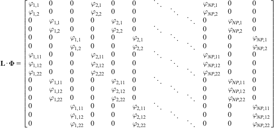
For convenience, Eq. (4.103) is rewritten in matrix form as follows:
(4.104)
where
(4.105)
(4.106)
 (4.106)
(4.107)
 (4.107)
(4.108)
(4.109)
(4.110)
(4.111)
Based on Eqs. (4.88) and (4.104), the estimated value can be calculated numerically as:
(4.112)
where
(4.113)
The approximation function ![]() can be expressed in the form of u(x):
can be expressed in the form of u(x):
(4.114)
 (4.114)
where ![]() is the interpolation function, which can be expressed by:
is the interpolation function, which can be expressed by:
(4.115)
(4.116)
(4.117)
(4.118)
where I is a n×n unit matrix. The first- and second-order derivatives of the shape function can be derived from Eq. (4.115):
(4.119)
(4.120)
where ![]() and
and ![]() denote the first- and second-order spatial derivatives, respectively. Compared with MLS approximation, the shape function
denote the first- and second-order spatial derivatives, respectively. Compared with MLS approximation, the shape function ![]() constructed using the MK interpolation in Eq. (4.115) has a distinct property:
constructed using the MK interpolation in Eq. (4.115) has a distinct property:
(4.121)
Fig. 4.20A illustrates the one-dimensional shape functions which demonstrate that the MK interpolation has the delta function property; first- and second-order derivatives of the shape function are plotted in Fig. 4.20A and C, respectively.


4.5.5 The Mesh-Free Computational Framework
The displacement of a deformed SWCNT is divided into two parts: the displacement of an undeformed SWCNT relative to the reference configuration and the displacement of the deformed SWCNT relative to the undeformed SWCNT. The first part can be exactly calculated (Fig. 4.21). The second part is approximated using the MLS approximation, i.e.,
(4.122)
 (4.122)
where ![]() is the nodal parameter,
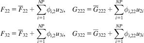
is the nodal parameter, ![]() is the mesh-free shape function, and NP is the number of nodes whose supports cover the evaluating point. It is noted that any node has 3 degrees of freedom, but the interpolation shape function is built on the 2-D domain (Fig. 4.22).
is the mesh-free shape function, and NP is the number of nodes whose supports cover the evaluating point. It is noted that any node has 3 degrees of freedom, but the interpolation shape function is built on the 2-D domain (Fig. 4.22).
The first- and second-order gradients are computed using the following formulas.
(4.123)
where ![]() and
and ![]() are the gradients of the evaluated point when no loading is applied, and can be analytically calculated using the mapping equation (4.56), and
are the gradients of the evaluated point when no loading is applied, and can be analytically calculated using the mapping equation (4.56), and ![]() and
and ![]() are approximated as
are approximated as
(4.124)
 (4.124)
with ![]() and
and ![]() , respectively, being the first- and second-order derivatives of the mesh-free shape function
, respectively, being the first- and second-order derivatives of the mesh-free shape function ![]() .
.
Newton’s method is used to solve the nonlinear governing equations in which the loading is decomposed into a series of time-steps, and at each iterative step the equilibrium state is determined by iteratively solving the incremental equation.
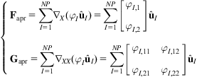
With the definition of the deformation gradient vector grad and the stress vector ![]() , the weak form of the equilibrium equation can be written as
, the weak form of the equilibrium equation can be written as
(4.125)
Newton’s method is adopted to solve the nonlinear governing equations. The stress at the n+1th iterative step can be obtained by:
(4.126)
Thus, Eq. (4.125) can be rewritten as:
(4.127)
At the n+1th iterative step,
(4.128)
(4.129)
Based on Eqs. (4.128) and (4.129), Eq. (4.127) can be rewritten as:
(4.130)
where ![]() and M is a combination of the tangential moduli which can be expressed as:
and M is a combination of the tangential moduli which can be expressed as:
(4.131)
Consequently, Eq. (4.130) can be expressed as:
(4.132)
The displacement increment of the evaluating point can be approximated as
(4.133)
 (4.133)
(4.134)
 (4.134)
(4.135)
 (4.135)
The gradient increment can be calculated as
(4.136)
(4.137)
 (4.137)
(4.138)
 (4.138)
The outward normal gradient is calculated as
(4.139)
Substituting Eqs. (4.133), (4.136), and (4.139) into (4.132), we have
(4.140)
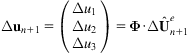
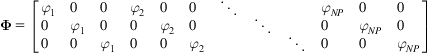
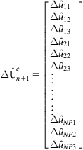
Thus, we can obtain the incremental system equation
(4.141)
where ![]() contains the nodal parameters of all of the mesh-free nodes. The global stiffness matrix is
contains the nodal parameters of all of the mesh-free nodes. The global stiffness matrix is
(4.142)
The nonequilibrium force vector is
(4.143)
(4.144)
(4.145)
Eq. (4.144) expresses the external forces. The stable state is obtained by iteratively solving Eq. (4.141) until f reaches zero.
4.5.6 Integration Scheme for a Discrete Equation
The evaluation of integrals in Eq. (4.142) requires an appropriate integral technique. In mesh-free methods, the evaluation of these integrations is a key point. Several integrations have been proposed in the literature.
One approach is to use the background mesh-free or background cell for quadrature integration, which is used in most mesh-free methods. In this approach, the domain is divided into a series of background cells, and the quadrature rule is used in each. Different from the FEM, the background cells are used only to implement the integration, and they need not be compatible with the mesh-free nodes. However, this approach is not very stable or accurate. The setup of the background cells and the distribution of the quadrature points at the global level do not ensure sufficient quadrature points in the compact support, which is crucial to the accuracy of the integration. It has been found that if quadrature integration is performed using background cells whose corners coincide with the nodes, then significant integration errors may occur in irregular cells. At the same time, if the background cells do not match the compact support of the mesh-free interpolations, then considerable integration errors may also arise. Nevertheless, this method is still widely used due to its simplicity both in theory and implementation. To alleviate integration error, one can use the integration cells that coincide with the nodal arrangements and apply a higher-order Gaussian quadrature, although this may result in significantly increased computational time. For example, 2×2 quadrature points can achieve a high level of accuracy, but the mesh-free method may require 4×4 quadrature points.
To avoid the “ghost” of the background cell, a nodal integration procedure was developed by Beissel and Belytschko [125]. This approach added a stabilization term consisting of the square of the residual of the equilibrium equation in the potential energy functional, and the resulting equations were integrated only at the nodes. However, introducing this additional term in the potential energy sacrifices variational consistency, and hence compromises the accuracy of the formulation.
Another development is the local support integration that was proposed by Li and Liu [126]. Due to the compact support of the mesh-free shape functions, effective integration should be performed for the common parts of the supports for the associated nodes. If each node takes on the same support shape, then we can fix the same quadrature rule for each support and integrate the weak form locally from one compact to another. By carrying out integration on the compact support, we are free from the background cell. One difficulty associated with local support integration is the integration of the compact that is cut by the boundary. A particular technique is needed for integration on these cut compacts because they are not regular. Moreover, in this approach, we still need to set up the quadrature points in the compact support.
To avoid the quadrature points completely, Chen et al. [84] put forward a stabilized conforming nodal integration method for the mesh-free Galerkin method. A smoothing stabilization technique was used to overcome the numerical instabilities occurring in the nodal integration.
From the above review, we can see that there are several integration strategies that can be used in the mesh-free method. However, in the present research, background quadrature meshes are used for integration due to their simplicity and easy implementation. The mesh-free nodes are collocated uniformly along the axial and circumferential directions, and the background cells are chosen to coincide with the nodal arrangements, i.e., each integral cell is a rectangle. The Gaussian quadrature rule is used for each cell. In the practical calculation, the Gaussian points can be globally marked. To avoid repeating the calculation for each Gaussian point, the information that includes the nodes whose supports cover the Gaussian points and the corresponding shape functions and their first- and second-order derivatives is calculated and deposited in advance. Assuming that the total number of Gaussian points for the entire problem domain is NQ, we can evaluate the stiffness matrix in Eq. (4.142) as follows.
(4.146)
where ![]() is the Gaussian weight. For each Gaussian point, we can obtain the substiffness matrix
is the Gaussian weight. For each Gaussian point, we can obtain the substiffness matrix
(4.147)
Global stiffness can be obtained by assembling all of these substiffness matrices.
4.5.7 Enforcement of Essential Boundary Conditions
In comparison with the FEM, the mesh-free method has an obvious difficulty: the imposition of essential boundary conditions. Similar to most of the mesh-free shape functions, the MLS shape functions lack the Kronecker delta property, i.e., ![]() . Thus, the approximation that is generated by the MLS method does not pass through the nodal parameter values:
. Thus, the approximation that is generated by the MLS method does not pass through the nodal parameter values:
(4.148)
where I and J denote the I-th and J-th mesh-free nodes, respectively. Therefore, the essential boundary conditions cannot be treated directly in mesh-free methods as they can in the FEM.
Some techniques have been proposed to impose the essential boundary conditions in mesh-free computations. Belytschko et al. [69] proposed the Lagrange multiplier method, in which not only the discrete field variables, but also the Lagrange multipliers, must be solved. Therefore, a separate set of interpolations for the Lagrange multipliers is required, which results in an increasing problem size. The introduction of the Lagrange multipliers to the method also leads to the singularity of the stiffness matrix, and thus a special solver is needed. Krongauz [127] introduced the EFG method coupled with the FEM method, in which finite elements are placed along the essential boundary so that the combined shape functions exactly satisfy the Kronecker delta property along the boundary. Ren and Liew [128] proposed the nodal interpolation method (NIM) and the direct imposition method (DIM). In the NIM, the polynomial interpolations are constructed near the essential boundary, and the combination of these interpolants with the mesh-free shape function allows the essential boundary conditions to be satisfied along the boundary. In the DIM, after a mathematical treatment is introduced to the resulting system matrix equations, the essential boundary conditions can be imposed directly as in the FEM. Chen et al. [85,91] developed a full transformation method, in which a global transformation matrix is introduced to transform the unknown variable vector and the stiffness matrix into those in the real deformation space. This method can achieve good efficiency and is very suitable to vibration problems. However, it is quite expensive. For nonlinear problems in particular, the repeated operations of the matrix multiplication requires a large amount of computational time. Zhu and Atluri [114] employ the penalty function method to impose the essential boundary conditions. The process in this method is similar to that in the FEM except that the mesh-free approximation at the boundary points is computed in advance. Other treatments of the essential boundary conditions include the Gram-Schmidt orthogonalization method [129], the singular weight function [130], and the development of the modified variational principle [115].
The full transformation method is found to be very accurate to impose the essential boundary conditions. However, the frequent matrix transformation often requires a large amount of computational resources for the present nonlinear problem. Therefore, the penalty function method was mainly used in preparing this thesis.
Assuming that the i-th displacement is prescribed at a boundary node ![]() , this given displacement can be interpolated with the MLS approximation as follows.
, this given displacement can be interpolated with the MLS approximation as follows.
(4.149)
where ![]() denotes a boundary node at which the i-th displacement is given,
denotes a boundary node at which the i-th displacement is given, ![]() is the prescribed displacement increment, and
is the prescribed displacement increment, and ![]() is the nodal parameter.
is the nodal parameter.
Eq. (4.149) is performed at all of the boundary nodes at which the essential boundary conditions are prescribed, and all of these equations can be assembled as
(4.150)
(4.151)
 (4.151)
where ![]() is determined by the index i of the prescribed displacement
is determined by the index i of the prescribed displacement ![]() at the boundary
at the boundary ![]() , and it takes
, and it takes ![]() (for i=1),
(for i=1), ![]() (for i=2) or
(for i=2) or ![]() (for i=3).
(for i=3).
The weak equilibrium equation is
(4.152)
 (4.152)
where α is the penalty number.
Using Eq. (4.150), the discretized equation can be obtained as
(4.153)
The displacement in the first step can be precisely calculated, while that in the second step is accomplished by using the MK interpolation:
(4.154)
where the matrix ![]() and the vectors
and the vectors ![]() and f are of the same form as Eq. (4.141).
and f are of the same form as Eq. (4.141).
4.5.8 Stability of the Algorithm
The stable state of the structures is determined by iteratively solving the incremental equation (4.141) with the nonequilibrium force and the stiffness matrix at each iterative step. The present algorithm is actually a standard Newton–Raphson method [131], which is faster than gradient-based methods, such as the conjugate gradient method [132] in which only the first-order derivative of the potential energy is required. However, the stiffness matrix ![]() may not be positive definite in some cases, such as when buckling and material softening occur; thus, the iterative solution does not converge to the minimum point of the potential energy. A simple way to remedy this problem is to replace
may not be positive definite in some cases, such as when buckling and material softening occur; thus, the iterative solution does not converge to the minimum point of the potential energy. A simple way to remedy this problem is to replace ![]() with
with ![]() , where I is the identity matrix, and
, where I is the identity matrix, and ![]() is a positive number. The repeated replacement can ensure that the solution converges to the real one. The stiffness matrix
is a positive number. The repeated replacement can ensure that the solution converges to the real one. The stiffness matrix ![]() generally becomes positive definite after a few cycles of replacement, and the standard Newton–Raphson method can then be resumed. This modification has been used in the atomic-scale finite element [133,134].
generally becomes positive definite after a few cycles of replacement, and the standard Newton–Raphson method can then be resumed. This modification has been used in the atomic-scale finite element [133,134].
The choice of ![]() should ensure that
should ensure that ![]() is positive definite. The ideal value of
is positive definite. The ideal value of ![]() is a positive number that is slightly larger than the magnitude of the most negative eigenvalue of
is a positive number that is slightly larger than the magnitude of the most negative eigenvalue of ![]() [131] because the larger the value of
[131] because the larger the value of ![]() , the slower the convergence of the solutions. Therefore, to achieve a good convergence rate, we can first calculate the eigenvalue of
, the slower the convergence of the solutions. Therefore, to achieve a good convergence rate, we can first calculate the eigenvalue of ![]() at each iterative step. However, the calculation of this eigenvalue consumes additional computational time. Therefore, for small-sized structures, the value of
at each iterative step. However, the calculation of this eigenvalue consumes additional computational time. Therefore, for small-sized structures, the value of ![]() can be chosen by calculating the eigenvalue of
can be chosen by calculating the eigenvalue of ![]() . For large-scale structures, it can be determined by frequent attempts.
. For large-scale structures, it can be determined by frequent attempts.
4.5.9 Procedures for Equilibrium Solution
Based on the above illustration, the solution procedure for a loading step can be summarized as follows (the MLS shape functions and their first- and second-order derivatives are calculated and deposited for each Gaussian point prior to the first loading step).
1. Compute the external force vector ![]() if the external force is prescribed on the boundary.
if the external force is prescribed on the boundary.
2. Compute the internal force vector ![]() based on the results of the above iteration step.
based on the results of the above iteration step.
3. Compute the nonequilibrium force ![]() .
.
4. Compute the stiffness matrix.
a. Compute ![]() at each Gaussian point.
at each Gaussian point.
i. Calculate F and G using the MLS approximation.
ii. Optimize the energy of the representative cell.
b. Assemble the global stiffness matrix ![]() .
.
5. Enforce the essential boundary conditions.
a. The first iteration step?
If yes, then displacement increment ![]() is applied.
is applied.
If no, then the displacement increment is set as ![]() .
.
6. Solve the equation system ![]() .
.![]() is positive definite?
is positive definite?
b. If no, then modify the stiffness matrix as ![]() .
.
7. Check if the convergence criterion is satisfied.
a. If yes, then go to the next loading step.
4.5.10 Validation Studies
The above computational strategy has been written in a standard code using the Fortran language. In the calculation, we use the internal routine DLSASF of Fortran software Powerstation 4.0 to solve the linear system of equations (i.e., Eqs. 4.141 and 4.153). In this section, two simple examples are provided to illustrate the validity of the developed mesh-free computational scheme. The mesh-free nodes are uniformly collocated along the circumferential and axial directions, and the background integral cells are in accordance with the nodal arrangements. In the future discussion, the nodal collation ![]() means that the n nodes are uniform along the circumferential direction and the m nodes are uniform along the axial direction. Here, we mainly check the convergence of the method and discuss the dependence of the solutions on the DOI (the scaling factor
means that the n nodes are uniform along the circumferential direction and the m nodes are uniform along the axial direction. Here, we mainly check the convergence of the method and discuss the dependence of the solutions on the DOI (the scaling factor ![]() ).
).
4.5.11 Uniform Tension
A tension test is first carried out. An (8, 8) SWCNT is considered, and it has 36 hexagonal cells along the axial direction. The total atom number is 1168, and the original length is 9.04 nm. In the numerical simulation, one end plane is fixed, and the tube is loaded by giving another end plane an axial movement at 0.1 nm per loading step. A total 10 loading times are applied during the test.
Different numbers of nodes and different values of ![]() are used in the tests. First, let us consider the convergence of solutions. The cases of
are used in the tests. First, let us consider the convergence of solutions. The cases of ![]() and
and ![]() are calculated. Shown in Tables 4.4 and 4.5 are the strain energy and axial stress when 10% axial strain is applied. Here, the axial stress is calculated as the sum of the nodal force on the end plane divided by the area of the cross-section that is evaluated as
are calculated. Shown in Tables 4.4 and 4.5 are the strain energy and axial stress when 10% axial strain is applied. Here, the axial stress is calculated as the sum of the nodal force on the end plane divided by the area of the cross-section that is evaluated as ![]() (R is the radius, and t=0.334 nm is the thickness of the tube). With the increasing number of nodes, an obvious convergence can be seen from Tables 4.4 and 4.5. To reveal the variation of the system energy versus the axial strain, the energy–strain curve is first plotted for the case of
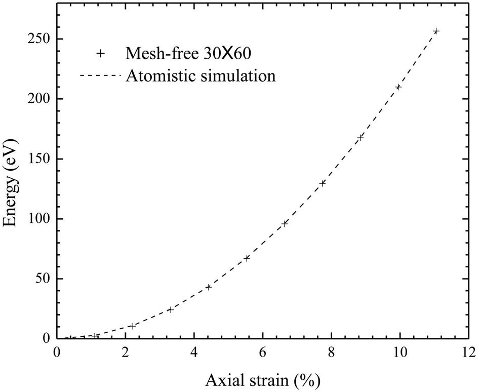
(R is the radius, and t=0.334 nm is the thickness of the tube). With the increasing number of nodes, an obvious convergence can be seen from Tables 4.4 and 4.5. To reveal the variation of the system energy versus the axial strain, the energy–strain curve is first plotted for the case of ![]() nodes with the use of
nodes with the use of ![]() along with the result that is obtained with the atomic simulation (see Fig. 4.23). The curves for the different numbers of nodes are so close that they cannot be clearly displayed in the same figure. A separate figure is provided to show the energy error in comparison with that obtained with the atomic simulation case (see Fig. 4.24). Here, the energy error refers to the calculated energy with the present nodes minus that obtained with the atomic simulation. From Tables 4.4 and 4.5 and Figs. 4.23 and 4.24, it can be seen that the results are very close to those of the atomic simulation even when
along with the result that is obtained with the atomic simulation (see Fig. 4.23). The curves for the different numbers of nodes are so close that they cannot be clearly displayed in the same figure. A separate figure is provided to show the energy error in comparison with that obtained with the atomic simulation case (see Fig. 4.24). Here, the energy error refers to the calculated energy with the present nodes minus that obtained with the atomic simulation. From Tables 4.4 and 4.5 and Figs. 4.23 and 4.24, it can be seen that the results are very close to those of the atomic simulation even when ![]() nodes are used, which indicates that continuum simulation can efficiently reduce the degrees of freedom of the problem. This is an important advantage of the continuum method.
nodes are used, which indicates that continuum simulation can efficiently reduce the degrees of freedom of the problem. This is an important advantage of the continuum method.
Table 4.4
Strain Energy and Axial Stress When 10% Axial Strain Is Applied. ![]() Is Fixed as 2.0
Is Fixed as 2.0
| Node Numbers | Energy (eV) | Stress (GPa) |
| 213.5231 | 67.7021 | |
| 211.7653 | 67.3328 | |
| 210.7685 | 67.1753 | |
| 210.2493 | 67.1385 | |
| 210.4371 | 67.1474 | |
| 210.0487 | 67.1273 |
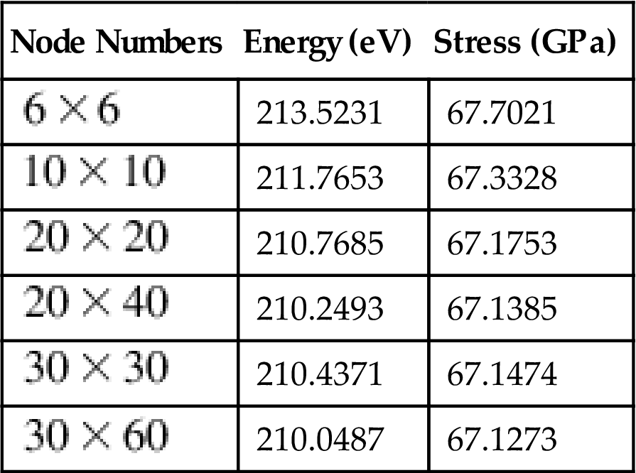
Table 4.5
Strain Energy and Axial Stress When 10% Axial Strain Is Applied
| Node Numbers | Energy (eV) | Stress (GPa) |
| 211.7094 | 67.2891 | |
| 210.9887 | 67.1708 | |
| 210.3914 | 67.1273 | |
| 209.9847 | 67.1149 | |
| 210.1466 | 67.1231 | |
| 209.8760 | 67.1115 |

 nodes.
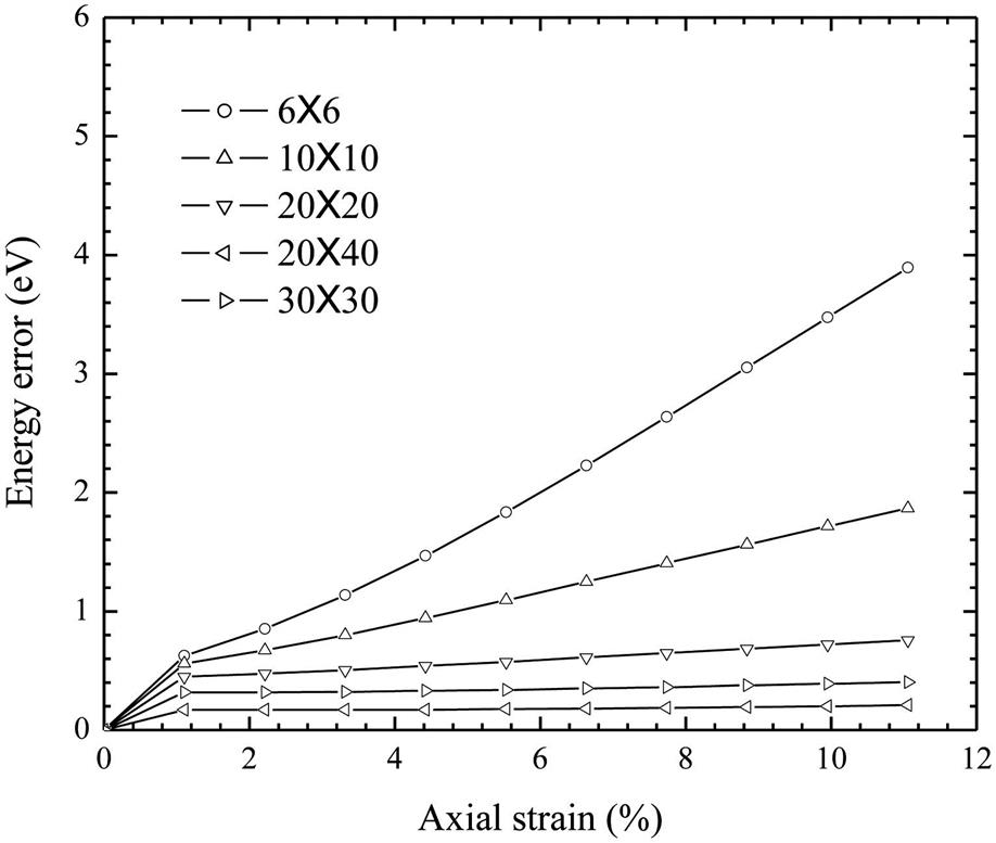
As illustrated before, the size of the compact support (DOI) generally has an effect on the computational results. The choice of the DOI depends on the properties of the practical problems. According to the literature, the efficient range of the scaling factor ![]() is typically 2.0–4.0. A series of computations have been performed to test the effects of
is typically 2.0–4.0. A series of computations have been performed to test the effects of ![]() . The results reveal that the different values of
. The results reveal that the different values of ![]() in the range of 2.0–4.0 do not provide significant differences in the final results for the present tension test. This phenomenon can be seen from Table 4.6, which shows the dependence of the system energy and axial stress on
in the range of 2.0–4.0 do not provide significant differences in the final results for the present tension test. This phenomenon can be seen from Table 4.6, which shows the dependence of the system energy and axial stress on ![]() .
.
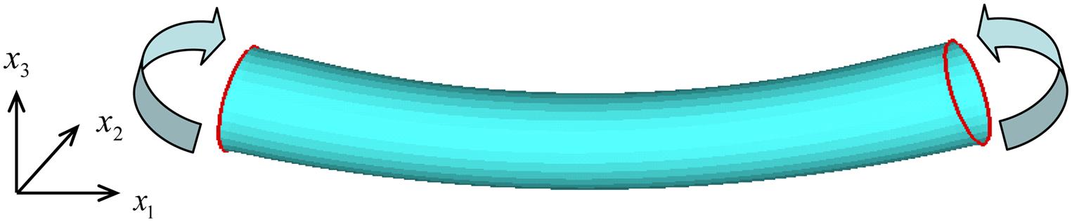
4.5.12 Bending Test
A bending test is carried out by incrementally rotating the two end planes of the SWCNTs in opposite directions (Fig. 4.25). During the rotation of the two end planes, the axial movement of one end is prohibited, but that of the other is unconstrained. A (15, 0) SWCNT is considered. It has 30 hexagonal cells along the axial direction, and the original length is 12.87 nm. The rotation angle is 1 degree per loading step, and a total of 21 steps are applied. The purpose of the present computations is to test the convergence of the solutions and the effect of the scaling factor ![]() .
.
First, ![]() is fixed as 2.0. Fig. 4.26 shows the variation of the system energy versus the bending angle for the cases of
is fixed as 2.0. Fig. 4.26 shows the variation of the system energy versus the bending angle for the cases of ![]() ,
, ![]() ,
, ![]() , and
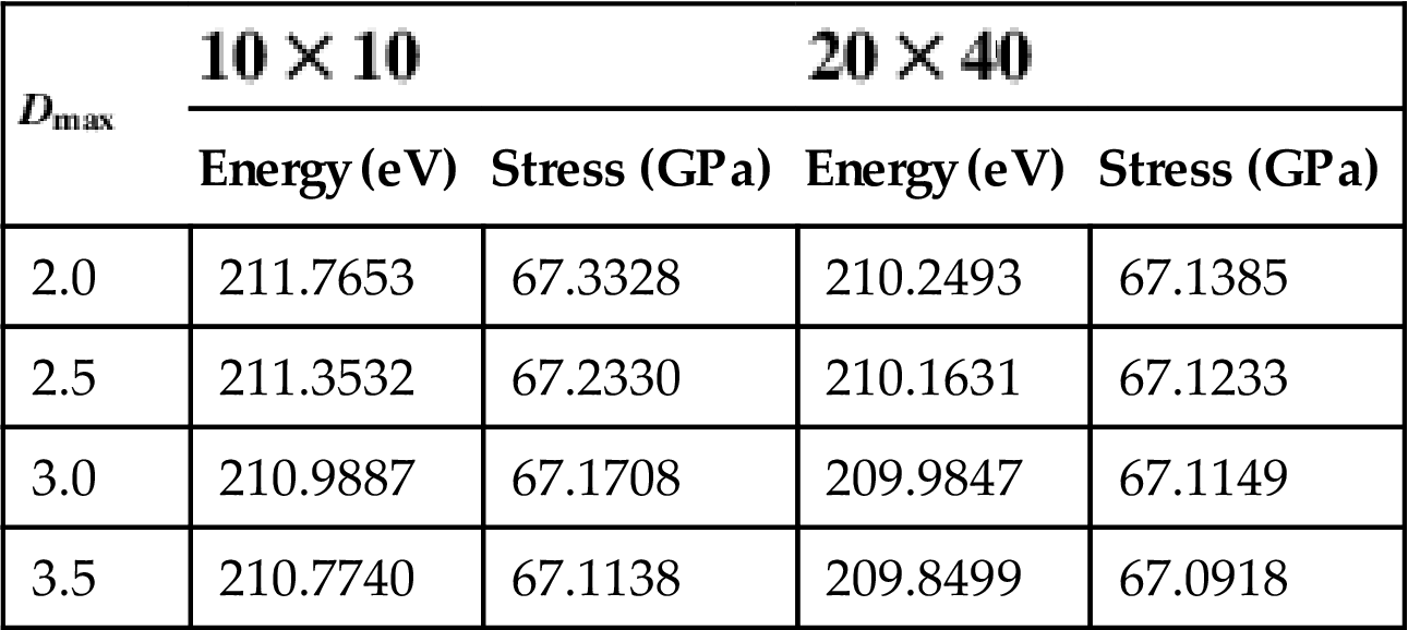
, and ![]() nodes. Good convergence can be seen. To check the effect of the DOI, detailed computations are carried out for Dmax=2.0, 2.5, 3.0, and 3.5. Table 4.7 shows the dependence of the solution on Dmax and the number of nodes. When fewer nodes are used, Dmax=2.0 has a bad result. However, when more nodes are used, Dmax in the range of (2.0, 3.0) does not show very large differences.
nodes. Good convergence can be seen. To check the effect of the DOI, detailed computations are carried out for Dmax=2.0, 2.5, 3.0, and 3.5. Table 4.7 shows the dependence of the solution on Dmax and the number of nodes. When fewer nodes are used, Dmax=2.0 has a bad result. However, when more nodes are used, Dmax in the range of (2.0, 3.0) does not show very large differences.
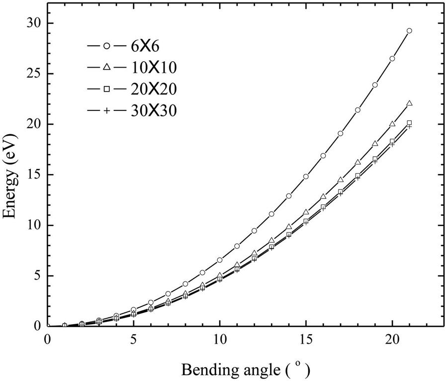
Table 4.7
The Dependence of the Strain Energy on the Scaling Factor and the Number of Nodes
| Node Numbers | Dmax=2.0 (eV) | Dmax=2.5 (eV) | Dmax=3.0 (eV) | Dmax=3.5 (eV) |
| 26.4863 | 19.2940 | 19.1104 | 19.0163 | |
| 19.9848 | 18.1101 | 18.1191 | 17.9542 | |
| 18.3417 | 17.9120 | 17.9631 | 17.8662 | |
| 18.3100 | 17.8917 | 17.9441 | 17.8388 | |
| 18.0450 | 17.8907 | 17.9241 | 17.8660 | |
| 18.0212 | 17.8756 | 17.8947 | 17.8037 |

4.6 Buckling and Postbuckling Behaviors
4.6.1 Hydrostatic Pressure-Induced Structural Transitions of SWCNTs
In the previous study, we obtain a pressure–radial strain curve for SWCNTs through a semianalytical method. In fact, the structural transition appears when the pressure reaches the critical value. A number of high-pressure experiments have been carried out on bundles of SWCNTs [135–137], and they show pressure-induced structural transition in the range of 1–2 GPa. Recent experiments have also shown that pressure may induce transitions in the electrical and magneto-transport properties of SWCNT bundles [138], which correlates closely with pressure-induced structural shape transition. In parallel, extensive theoretical studies, ranging from first-principle calculations [139–141] and molecular dynamic simulation [142,143] to continuum mechanics modeling [144], have been performed by several groups to study the properties of both isolated single SWCNTs and bundles of SWCNTs under hydrostatic pressure. For an isolated single SWCNT, it has been shown that pressure induces a series of shape transitions, transforming its cross-sections from a circle to an elliptical and then a peanut shape [142,144]. In this section, we employ the mesh-free method to study the structural transition of an isolated single SWCNT.
As introduced before, the mesh-free formulation is based on the transformation from a planar sheet (2-D) to a spatial curved surface (3-D). When hydrostatic pressure is applied on an SWCNT, it uniformly deforms along the axial direction, and we need only consider the change of its cross-section. Thus, an SWCNT can be simplified as a circle, and its counterpart in the reference configuration is a straight line segment (see Fig. 4.27). In the simulation, this line segment (Fig. 4.27A) serves as the reference configuration, and the initial undeformed circle (Fig. 4.27B) can be formed by rigidly rolling up the line segment into a circle. The length of the line segment is ![]() , and the cell structure in the reference configuration should be determined with the method described in Section 4.1. The deformation from the reference configuration to the current configuration (Fig. 4.27C) can be divided into two parts: one is from the line segment to the circle, and the other is from the circle to the current configuration. The first part can be calculated exactly. The displacement of the current configuration relative to the initial circle can be completely expressed with
, and the cell structure in the reference configuration should be determined with the method described in Section 4.1. The deformation from the reference configuration to the current configuration (Fig. 4.27C) can be divided into two parts: one is from the line segment to the circle, and the other is from the circle to the current configuration. The first part can be calculated exactly. The displacement of the current configuration relative to the initial circle can be completely expressed with ![]() and
and ![]() , and we only need to consider the gradient components
, and we only need to consider the gradient components ![]() ,
, ![]() ,
, ![]() , and
, and ![]() that can be calculated with
that can be calculated with ![]() and
and ![]() . It should be noted that with the radial deformation of an SWCNT a slight axial strain takes place, and this axial strain can be described with
. It should be noted that with the radial deformation of an SWCNT a slight axial strain takes place, and this axial strain can be described with ![]() . Moreover, a twisting angle may also occur, and this can be described with
. Moreover, a twisting angle may also occur, and this can be described with ![]() . Therefore, the energy of the representative cell is determined by
. Therefore, the energy of the representative cell is determined by ![]() ,
, ![]() ,
, ![]() ,
, ![]() ,
, ![]() , and
, and ![]() , and the strain energy density is a function of
, and the strain energy density is a function of ![]() ,
, ![]() ,
, ![]() ,
, ![]() ,
, ![]() , and
, and ![]() :
:
(4.155)

 . The deformation from the reference to the current configuration is divided into two parts.
The first- and second-order derivatives of ![]() with respect to
with respect to ![]() ,
, ![]() ,
, ![]() ,
, ![]() ,
, ![]() , and
, and ![]() can be calculated as described before.
can be calculated as described before.
The stable configurations of the system are identified with the minimization of the total energy, as follows.
(4.156)
where p is the hydrostatic pressure applied on the outside surface of an SWCNT, and ![]() is the normal displacement
is the normal displacement
(4.157)
where ![]() is the angle between the radius and the axis
is the angle between the radius and the axis ![]() .
.
The integral in Eq. (4.156) is performed along the circle, and E should be understood as the energy per unit length of SWCNTs.
In the mesh-free simulation, a series of nodes is collocated on the line segment (these can also be viewed as being on the undeformed circle). The displacement relative to the undeformed circle is approximated as
(4.158)
where ![]() is the 1-D mesh-free shape function that is defined on the line segment,
is the 1-D mesh-free shape function that is defined on the line segment, ![]() and
and ![]() are the nodal parameters, and NP is the number of nodes whose supporting domain covers the evaluated point. The deformation gradients are approximated as
are the nodal parameters, and NP is the number of nodes whose supporting domain covers the evaluated point. The deformation gradients are approximated as
(4.159)
 (4.159)
where ![]() ,
, ![]() ,
, ![]() , and
, and ![]() are the gradients of the undeformed circle and can be calculated exactly and
are the gradients of the undeformed circle and can be calculated exactly and ![]() and
and ![]() are the first- and second-order derivatives of
are the first- and second-order derivatives of ![]() with respect to
with respect to ![]() .
.
Assuming that the total N nodes are used, the total unknown vector can be written as
(4.160)
The nonequilibrium force and the stiffness matrix can be calculated as
(4.161)
The equilibrium configurations can be obtained by iteratively solving ![]() until f reaches zero. Moreover, around the structural transitions, the stiffness becomes nonpositive definite.
until f reaches zero. Moreover, around the structural transitions, the stiffness becomes nonpositive definite.
The numerical simulations are first carried out for a (10, 10) SWCNT. The computations reveal that the SWCNT displays the first structural transition when the hydrostatic pressure reaches a critical value. At this critical pressure, the cross-section transforms from a circle to an ellipse (see Fig. 4.28). The present computation reveals that 15 nodes can achieve good convergence prior to the structural transition. However, the critical pressure has a larger dependence on the node number. Given in Table 4.8 is the first critical pressure obtained for the different nodes when ![]() is fixed as 3.0. This suggests that more than 50 nodes should be used along the line segment to obtain an ideal critical pressure. Table 4.9 shows the dependence of the critical pressure on the scaling factor
is fixed as 3.0. This suggests that more than 50 nodes should be used along the line segment to obtain an ideal critical pressure. Table 4.9 shows the dependence of the critical pressure on the scaling factor ![]() when 60 nodes are used, which indicates that 2.5, 3.0, and 4.0 result in almost the same critical pressure, which confirms that a fewer number of nodes can achieve a good solution as discussed before.
when 60 nodes are used, which indicates that 2.5, 3.0, and 4.0 result in almost the same critical pressure, which confirms that a fewer number of nodes can achieve a good solution as discussed before.

Table 4.8
The First Critical Pressure Obtained With Different Nodes When ![]() Is Fixed as 3.0
Is Fixed as 3.0
| Number of Nodes | Critical Pressure (GPa) |
| 20 | 1.968 |
| 30 | 1.424 |
| 40 | 1.248 |
| 50 | 1.174 |
| 60 | 1.168 |
Table 4.9
The Dependence of the First Critical Pressure on ![]() When 60 Mesh-Free Nodes Are Used
When 60 Mesh-Free Nodes Are Used
| Critical Pressure (GPa) | |
| 2.0 | 1.216 |
| 2.5 | 1.177 |
| 3.0 | 1.168 |
| 3.5 | 1.170 |

Here, the long and short axes of the ellipse are used to describe the deformation. After the first structural transition, it is found that the length of the long axis increases with the increasing pressure, but the short axis reduces its length (see Figs. 4.28 and 4.29). At a pressure of 1.3 GPa, the second structural transition occurs, and the cross-section of the tube transforms from an elliptical to a peanut shape (see Fig. 4.28). When the pressure further increases, the short axis continues to reduce its length, but the length of the long axis remains almost unchanged. Fig. 4.28 shows the change of the cross-section at several pressure values. Fig. 4.29 shows the variation of the long and short axes with the pressure (prior to the first structural transition, the cross-section is a circle, and the two axes have the same lengths). To reveal the dependence of the critical pressure of the first structural transition on the chirality and radius of the CNTs, computations are carried out for (n, 0), (n, n), and (3n, 2n) SWCNTs with different radii. Fig. 4.30 plots the variation of the first transition pressure versus the tube radius for (n, 0), (n, n), and (3n, 2n) SWCNTs. It is found that the first transition pressure has almost no dependence on the chirality of the CNTs.


4.6.2 Axial Buckling of SWCNTs
This section considers the mechanical response of SWCNTs under axial compression. The axial buckling of CNTs has been studied by many researchers. In continuum-based analysis, the attention is generally focused on a prediction of the critical strain. The present research presents a complete numerical simulation of buckling behavior.
In the compression simulation, one end of the SWCNT is completely fixed, and the in-plane displacement of the other end is prohibited. Axial compressive displacement is applied at the free end, the stable state is solved, and then the further compressive displacement is applied. In the present simulation, the penalty function method [114] is used to enforce the essential boundary condition.
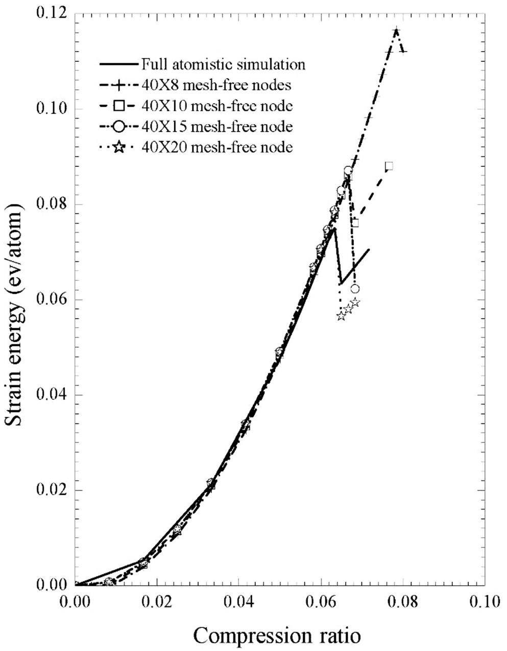
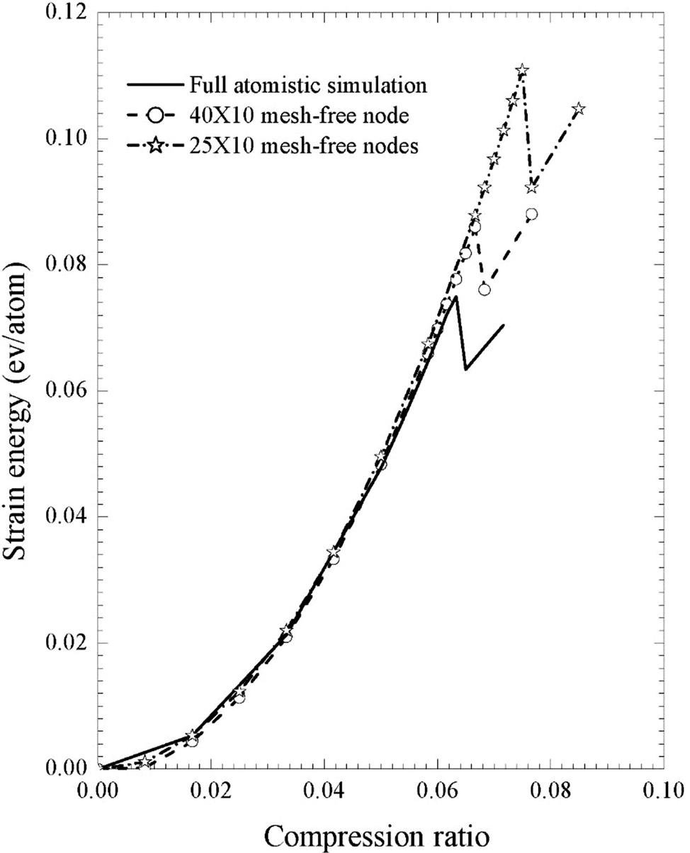
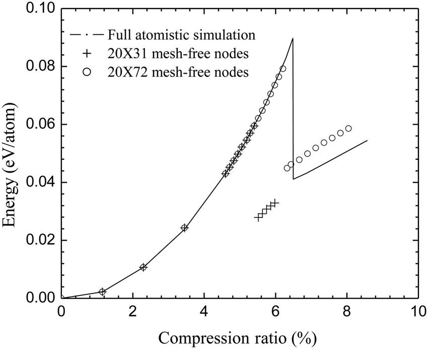
Using the present mesh-free method, we have simulated the compression of an (18, 0) SWCNT. It has 20 hexagonal cells along the axis, and its initial length is 8.71 nm (this value is obtained by initializing the undeformed tube using the atomic simulation). The problem is treated as quasistatic. The length of the tube is reduced by 0.1 nm per loading step at the early stage and 0.01 nm per loading step near to the buckling. To test the effect of the number of mesh-free nodes on the simulation result, different numbers of nodes have been used in the computation. Similar to the numerical tests discussed before, even ![]() nodes present a good simulation prior to buckling. However, the number of nodes has a large effect on the buckling strain. Fig. 4.31 plots the average energy per atom versus the compression ratio for the cases of
nodes present a good simulation prior to buckling. However, the number of nodes has a large effect on the buckling strain. Fig. 4.31 plots the average energy per atom versus the compression ratio for the cases of ![]() and
and ![]() nodes, along with the results of the full atomic simulation. A distinct energy jump appears at all three curves in Fig. 4.31, which corresponds to the buckling of the CNT. Prior to buckling, the compression ratio–energy curve is a quadratic curve, but afterwards, it is almost a straight line. From Fig. 4.31, it can be seen that the calculated energy in the cases of
nodes, along with the results of the full atomic simulation. A distinct energy jump appears at all three curves in Fig. 4.31, which corresponds to the buckling of the CNT. Prior to buckling, the compression ratio–energy curve is a quadratic curve, but afterwards, it is almost a straight line. From Fig. 4.31, it can be seen that the calculated energy in the cases of ![]() and
and ![]() is very precise prior to buckling. However, the number of nodes has a larger effect on the compression ratio of the buckling. Buckling occurs at a smaller compression ratio when a fewer number of nodes are used, and the comparison ratio of buckling tends to that of the full atomic simulation with an increasing number of nodes. Moreover, our computation also reveals that the compression ratio of buckling hardly changes if we fix the number of nodes along the longitudinal direction but increase it along the circumferential direction. This phenomenon can be explained by the fact that the drastic deformation is mainly along the axial direction for the compression test. Fig. 4.31 also shows that, even for the case of
is very precise prior to buckling. However, the number of nodes has a larger effect on the compression ratio of the buckling. Buckling occurs at a smaller compression ratio when a fewer number of nodes are used, and the comparison ratio of buckling tends to that of the full atomic simulation with an increasing number of nodes. Moreover, our computation also reveals that the compression ratio of buckling hardly changes if we fix the number of nodes along the longitudinal direction but increase it along the circumferential direction. This phenomenon can be explained by the fact that the drastic deformation is mainly along the axial direction for the compression test. Fig. 4.31 also shows that, even for the case of ![]() nodes, the energy calculation becomes less accurate after buckling. This is unsurprising because the deformation becomes drastically inhomogeneous, and it is difficult for the continuum method to capture microscale energy changes.
nodes, the energy calculation becomes less accurate after buckling. This is unsurprising because the deformation becomes drastically inhomogeneous, and it is difficult for the continuum method to capture microscale energy changes.
The buckling deformation obtained with ![]() nodes is shown in Fig. 4.32 along with that obtained with the full atomic simulation. The comparison shows that the present model can truly display the buckling pattern. Employing the mesh-free method, we also simulated the compression of the same SWCNT with the constitutive relations based on the standard Cauchy–Born rule, and the buckling deformation obtained is shown in Fig. 4.32C as a series of ridges scattered on the surface of the CNT. Obviously, this is a nonphysical buckling pattern, and it is the response of the structure in the case of no bending stiffness. The comparison shows that the model based on the standard Cauchy–Born rule does not describe the bending effect and thus cannot truly display the buckling behavior of CNTs. The present higher-order gradient theory considers the effect of the second deformation gradient, and thus the established model is more reasonable.
nodes is shown in Fig. 4.32 along with that obtained with the full atomic simulation. The comparison shows that the present model can truly display the buckling pattern. Employing the mesh-free method, we also simulated the compression of the same SWCNT with the constitutive relations based on the standard Cauchy–Born rule, and the buckling deformation obtained is shown in Fig. 4.32C as a series of ridges scattered on the surface of the CNT. Obviously, this is a nonphysical buckling pattern, and it is the response of the structure in the case of no bending stiffness. The comparison shows that the model based on the standard Cauchy–Born rule does not describe the bending effect and thus cannot truly display the buckling behavior of CNTs. The present higher-order gradient theory considers the effect of the second deformation gradient, and thus the established model is more reasonable.

Based on the present atomistic-continuum simulation, the deformation of SWCNTs can be analyzed from the perspective of a continuum. Fig. 4.33 shows the contour plots of the axial and circumferential strains and the strain energy density (the energy per unit area) just after the buckling occurs. The axial and circumferential strains are calculated as
(4.162)
 (4.162)

From Fig. 4.33, it can be seen that the deformation and energy are highly concentrated on the local kinking region. This may explain the phenomenon: the compression ratio–energy curve is straight after buckling, but a quadratic curve prior to buckling. There is maximum axial tensile strain at the convex regions, but the circumferential strain is negative. The distribution of the strain energy is similar to that of the axial strain, i.e., the maximum strain energy density is at the zone in which the axial tensile strain is largest.
4.6.3 Torsional Buckling of SWCNTs
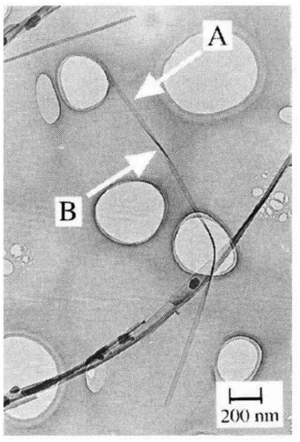
The torsional collapse of CNTs has been found in experimental investigations [145,146] (see Fig. 4.34) and has been modeled by MD [147] and other simulation methods [17]. The cross-section of a CNT remains a circle for the small twisting angle, but collapses when the twisting angle reaches a critical value.
In the modeling of twisting, the cross-sectional circular shape of the two ends of a CNT remains unchanged, and the twisting deformation is imposed by twisting the two ends in opposite directions without the prohibition of axial displacement.
A (10, 10) SWCNT is chosen for the twisting test. It has 47 hexagonal cells along the axis, and its initial length is 11.81 nm. The applied twisting angle is 1 degree per step. Plotted in Fig. 4.35 are the changes of the average energy per atom versus the twisting angle for the cases of ![]() and
and ![]() mesh-free nodes in a comparison with a full atomic simulation. When
mesh-free nodes in a comparison with a full atomic simulation. When ![]() nodes are used, the buckling angle is very close to that obtained by the full atomic simulation, whereas the buckling takes place at a larger twisting angle in the case of
nodes are used, the buckling angle is very close to that obtained by the full atomic simulation, whereas the buckling takes place at a larger twisting angle in the case of ![]() nodes. Similar to the compression test, a fewer number of nodes can provide a good simulation for the homogeneous deformation stage, but more nodes must be used to capture the critical twisting angle accurately. Moreover, the computations reveal that the critical twisting angle hardly changes if we fix the number of nodes along the circumferential direction but increase it along the longitudinal direction. This shows that the number of nodes along the circumferential direction has a large effect on the precision of the twisting simulation.
nodes. Similar to the compression test, a fewer number of nodes can provide a good simulation for the homogeneous deformation stage, but more nodes must be used to capture the critical twisting angle accurately. Moreover, the computations reveal that the critical twisting angle hardly changes if we fix the number of nodes along the circumferential direction but increase it along the longitudinal direction. This shows that the number of nodes along the circumferential direction has a large effect on the precision of the twisting simulation.
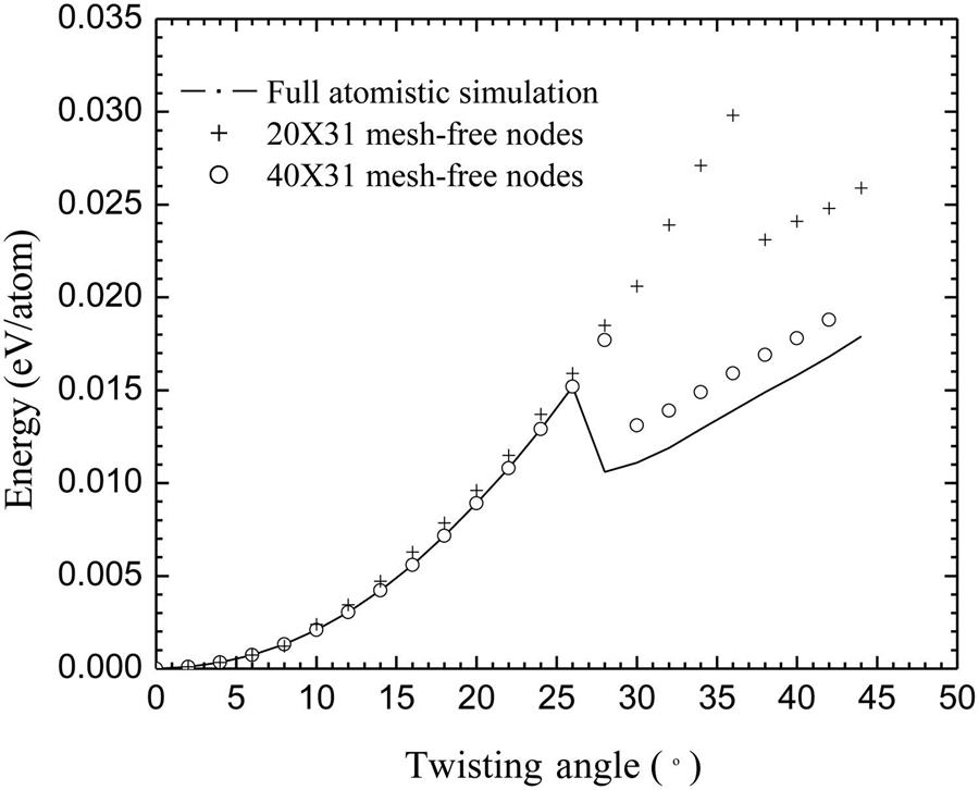
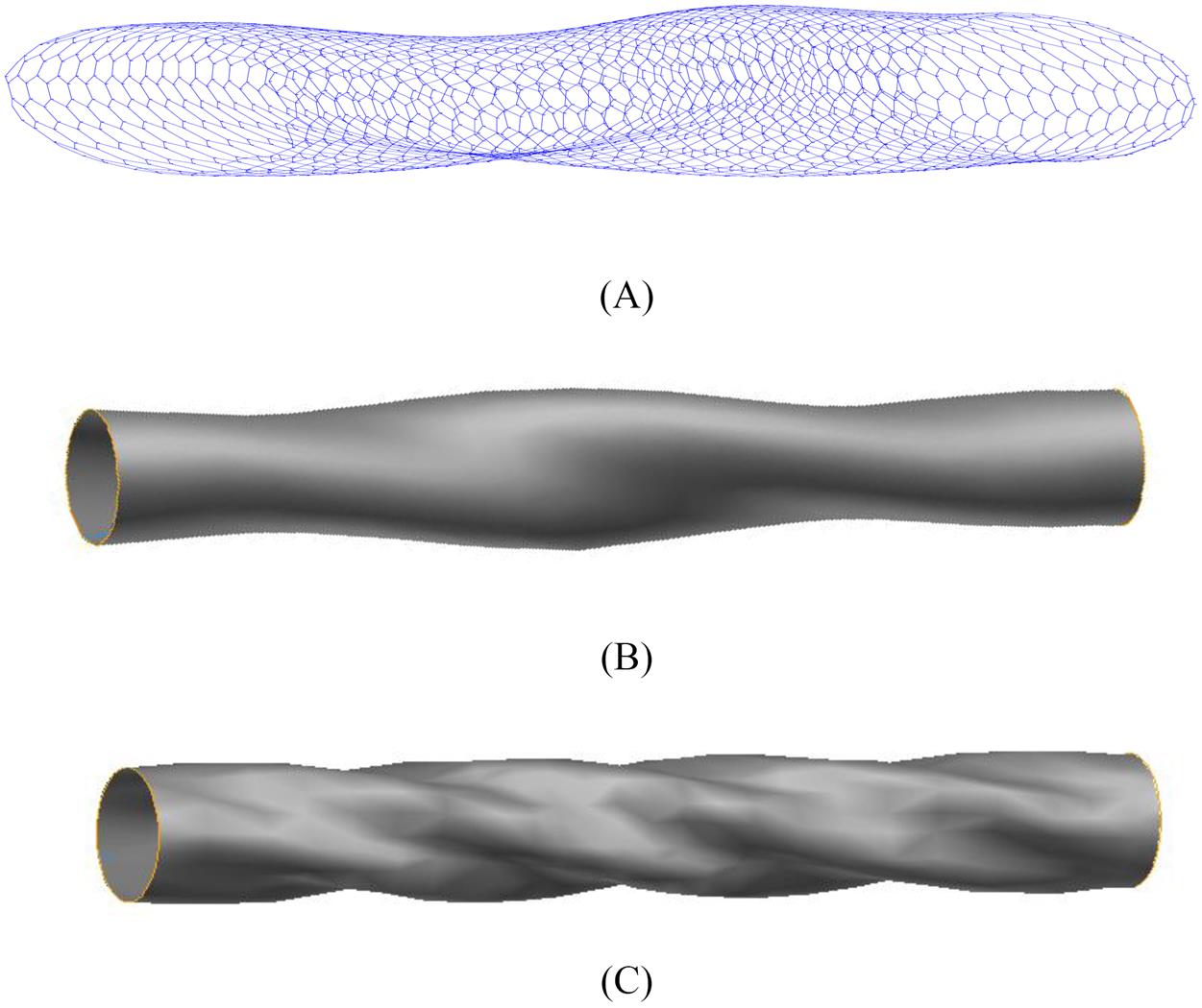
Fig. 4.36 shows a comparison of the twisting buckling patterns obtained with ![]() nodes and the full atomic simulation, which demonstrates that such patterns can be truly displayed with the present model. Moreover, we also perform the torsion test with the constitutive model based on the standard Cauchy–Born rule, and the simulated buckling deformation is shown in Fig. 4.36C. The deformation obtained is a nonphysical buckling pattern. This further demonstrates that the present model can accurately describe the constitutive response of CNTs, whereas the model based on the standard Cauchy–Born cannot.
nodes and the full atomic simulation, which demonstrates that such patterns can be truly displayed with the present model. Moreover, we also perform the torsion test with the constitutive model based on the standard Cauchy–Born rule, and the simulated buckling deformation is shown in Fig. 4.36C. The deformation obtained is a nonphysical buckling pattern. This further demonstrates that the present model can accurately describe the constitutive response of CNTs, whereas the model based on the standard Cauchy–Born cannot.
The deformation of a twisted SWCNT is now analyzed from the perspective of a continuum. Fig. 4.37 shows the contour plots of the shear strain, axial and circumferential strains, and strain energy density at a twisting angle of 22 degrees. The axial and circumferential strains are calculated using Eqs. (4.162), and the shear strain is calculated as
(4.163)
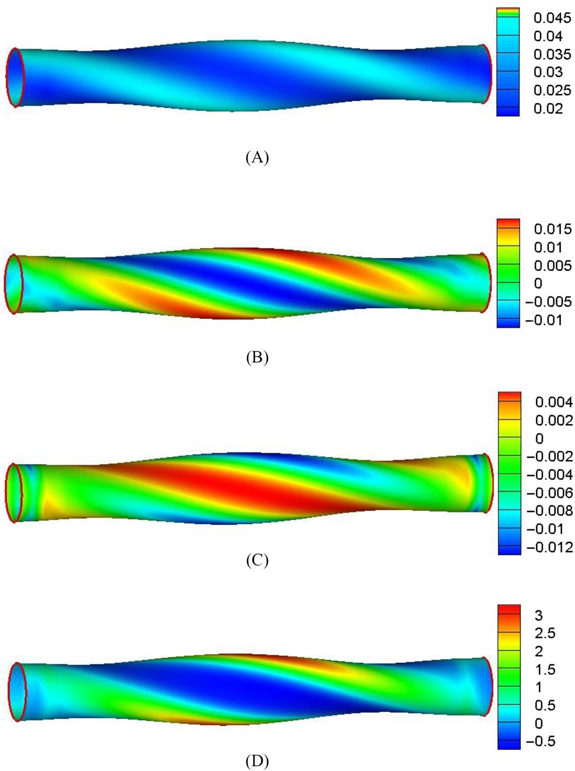
From Fig. 4.37, it can be seen that the distribution of the deformation and energy shows a series of twisted bands on the surface of the SWCNT. The large shear strain and axial tensile strain are distributed at the convex regions, and the large circumferential strain is distributed at the concave region. The distribution of the sreain energy is similar to that of the axial strain, i.e., the maximum strain energy density is at the zone in which the axial tensile strain is largest.
4.6.4 Buckling Behavior of SWCNTs Upon Bending
Due to the special structure of CNTs, bending buckling may be the type of buckling behavior that occurs most easily in CNTs in practice. In this section, the buckling behavior of SWCNTs upon bending is simulated and discussed in detail.
In most bending simulations of CNTs [147–149], the bending angle is imposed by incrementally rotating the two end planes in opposite directions. Both end sections remain circular and perpendicular to the deformed axis at each displacement increment. Because the axis is bent into a curve, the distance between the two end planes decreases with an increase in the rotating angle. The way to control this distance is not clearly specified in most of the literature. In [148], the researchers assume that an SWCNT takes on pure bending deformation, similarly to a beam under such loading conditions, and thus that the axis keeps a circular arc with its length being equal to the original length of the tube. The change in the distance between the two end sections is calculated exactly and imposed as the boundary condition. We can also treat this distance as an unknown and determine it by solving the equilibrium state of the tube. The detailed implementation is described as follows. At each loading step, the tube is bent by rotating the two end planes in opposite directions with respect to an axis that is perpendicular to the tube axis of the undeformed CNT and passing through its center. The rotating axis of one end plane is completely fixed, and the axial movement of the other end plane is not prohibited. Its axial position is treated as an unknown, and is determined with the minimization of the potential energy of the system along with the internal nodal unknowns. The above two methods of imposing bending deformation are respectively marked as the mode I and II loading methods. The latter method is mainly used in the present work, but the results of both methods are compared and discussed.
4.6.4.1 Bending buckling
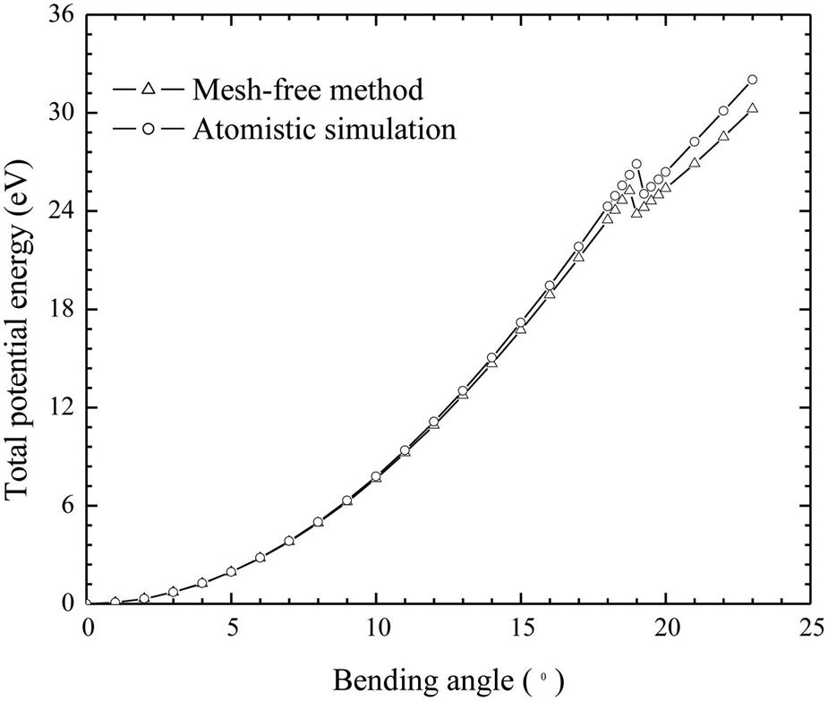
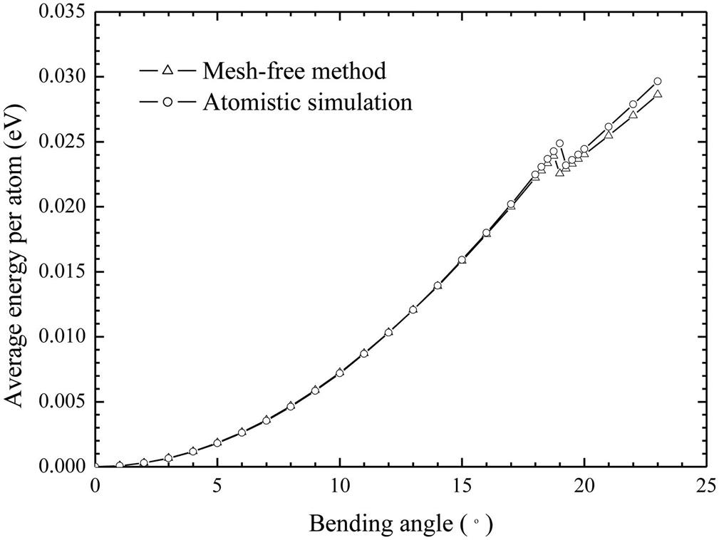
A (15, 0) SWCNT is considered first. It has 18 hexagonal cells along the axis of the tube, and the original equilibrium length is 7.65 nm. The mode II loading method is used, and the two end planes of the tube are reversely rotated 1 degree per loading step at the early stage and 0.25 degree per loading step around the buckling. Fig. 4.38 plots the change in the total energy along with the result that is obtained with the atomic simulation. Fig. 4.38 indicates that the energy difference between the two methods becomes large with an increasing bending angle. Plotted in Fig. 4.39 is the change in the average energy per atom, which is equal to the total energy divided by the atom number. The atom number is 1080 for atomic simulation, whereas, in the mesh-free method, the total number of atoms should be understood from the continuum concept and is taken as ![]() , where S is the surface area of the undeformed CNT, and
, where S is the surface area of the undeformed CNT, and ![]() is the average area per atom (
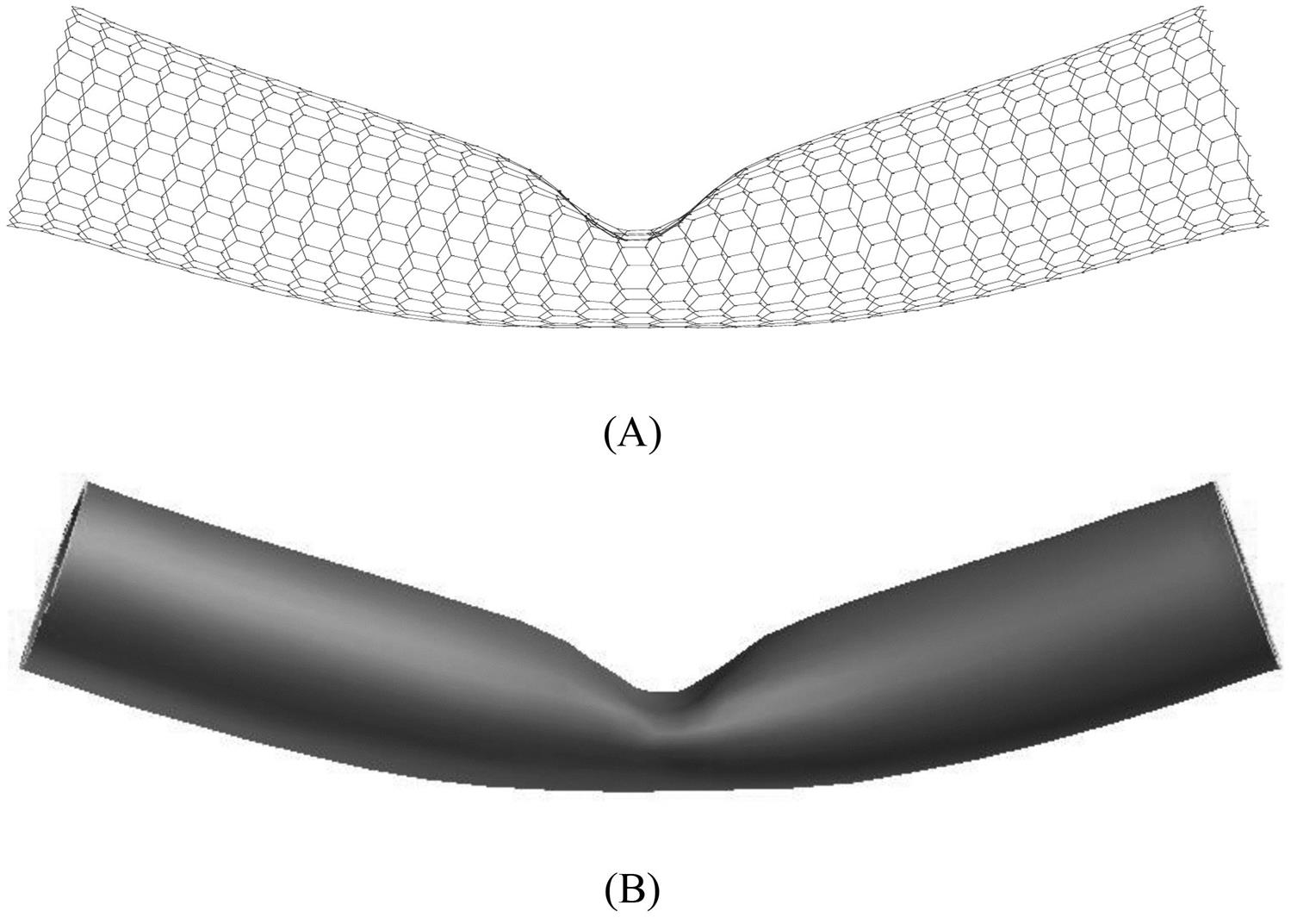
is the average area per atom (![]() denotes the bond length). Fig. 4.39 reveals that the average energy per atom in the two methods agrees well. A distinct energy jump that corresponds to the SWCNT buckling appears at the energy curves of the two methods. The buckling bending angles in the atomic simulation and in the mesh-free method are 19.25 and 19 degrees, respectively, which are very close. Fig. 4.40 shows the buckling deformations for the two methods, and it can be seen that the buckling patterns are very similar.
denotes the bond length). Fig. 4.39 reveals that the average energy per atom in the two methods agrees well. A distinct energy jump that corresponds to the SWCNT buckling appears at the energy curves of the two methods. The buckling bending angles in the atomic simulation and in the mesh-free method are 19.25 and 19 degrees, respectively, which are very close. Fig. 4.40 shows the buckling deformations for the two methods, and it can be seen that the buckling patterns are very similar.
We also perform the bending test on a longer (15, 0) CNT with a length of 30 hexagonal cells (12.87 nm). As plotted in Fig. 4.41, the change in the average bending energy shows good agreement with that in the full atomic simulation. The buckling angles in the atomic simulation and in the mesh-free method are ![]() and
and ![]() degrees, respectively. Fig. 4.42 provides a comparison of the buckling deformations of the two methods. Unlike in the short SWCNT, two symmetrical snap buckles are displayed in the long SWCNT.
degrees, respectively. Fig. 4.42 provides a comparison of the buckling deformations of the two methods. Unlike in the short SWCNT, two symmetrical snap buckles are displayed in the long SWCNT.