Classical Molecular Dynamics Simulations
Abstract
Classical molecular dynamics simulation as one of the typical atomistic simulations is widely and successfully used in the study of mechanical properties of carbon nanotubes (CNTs). The basic concept of this method is to simulate the time evolution of a system. It describes a system’s atomic-scale dynamics, in which atoms and molecules move while interacting with many of the other atoms and molecules in the vicinity. Brenner potential and the second-generation reactive empirical bond order potential are given to reflect carbon atomic interaction. Firstly, Young’s moduli of CNTs with impurities are extracted and reconstructions of tube with vacancy are investigated. Then buckling, fracture behavior, and thermal stability behaviors, under axial compression and tension, torsion, are simulated for perfectly structured CNTs, tube bundles, and coaxial CNTs inside a boron–nitride nanotube.
Keywords
Molecular dynamics; Brenner potential; reactive empirical bond order potential; Young’s moduli; impurities; reconstructions; buckling; fracture; thermal stability
3.1 Introduction
Ever since Iijima discovered carbon nanotubes (CNTs) in 1991 by using high-resolution transmission election microscopy [1] and, in particular, after they were successfully synthesized in 1993 by Bethune et al. [2], and Iijima and Ichihashi [3], CNTs have attracted considerable attention. CNTs are a new type of carbon material with very broad prospects [4–6] because of their unique structure and excellent physical and chemical properties. In particular, their excellent mechanical properties have aroused widespread interest in the scientific community, and progress [7–10] has been made in applying them to toughen materials. As the excellent mechanical properties of CNTs are likely to be related to their structure, much research attention in recent years has been paid to their structural properties and applications [7–17]. Recent studies have indicated that CNTs possess an exceptionally high elastic modulus [12,18] and can sustain large elastic and failure strains [19,20]. CNTs have thus been identified as a promising superfiber for nanotube-composite materials. As the excellent mechanical properties of CNTs are likely to be related to their structure, much research attention in recent years has been paid to their structural properties and applications.
Molecular dynamics (MD) simulation is by far the most popular tool for investigating the mechanical properties of CNTs. For example, Yakobson et al. [11] investigated axially compressed armchair single-walled carbon nanotubes (SWCNTs) using MD simulations and compared the solutions with those obtained from a simple continuum thin shell model. They observed that the continuum shell models can predict the buckling properties of SWCNTs satisfactorily provided that the mechanical parameters, such as the Young’s modulus and effective wall thickness, are judiciously adopted. Wang et al. [12] used MD simulation to study the elastic response and buckling modes of SWCNTs under axial compression. Cornwell and Wille [21] used MD simulation to study the response of a set of armchair SWCNTs and calculated the Young’s modulus of the tubes. Srivastava et al. [22] performed a MD simulation to examine the nanoplasticity of zigzag CNTs under compression. Recently, Liew et al. [13–17] studied the mechanical properties of armchair and zigzag SWCNTs and multiwalled carbon nanotubes (MWCNTs) composed of multiple armchair SWCNTs with different diameters. Wang et al. [12] applied MD simulation to study the elastic response and buckling modes of SWCNTs under axial compression.
3.2 Computational Model
Compared to the first-principle quantum mechanics, classical MD simulation is an empirical method which is easy to implement in large systems (millions to billions of atoms). The classical MD method was first proposed by Alder and Wainwright [23]. Up to now, MD simulation is the most popular tool for investigating the mechanical properties and structural deformation of CNTs. The basic concept of the method is to simulate the time evolution of a system. It describes a system’s atomic-scale dynamics, in which atoms and molecules move while interacting with many of the other atoms and molecules in the vicinity. The method relies on a mathematical description of total energy of the system as a function of all of atomic coordinates. Atoms in the system are treated as point-like masses that interact with each other according to a given potential energy E(r1, r2,…,rN), where rj is the vector position of the jth atom. The evolution is computed at every time-step, and the instantaneous location and velocity of each atom are then determined by solving Hamilton’s classical equation of motion from Newton’s second law.
(3.1)
where ![]() and
and ![]() are the mass and spatial coordinates of the ith atom, respectively, E is the empirical potential for the system, and ∇ denotes the spatial gradient. Due to the small scale involved, explicit integration algorithms, such as the Verlet method [24] and other high-order methods, are commonly used to ensure a high order of accuracy.
are the mass and spatial coordinates of the ith atom, respectively, E is the empirical potential for the system, and ∇ denotes the spatial gradient. Due to the small scale involved, explicit integration algorithms, such as the Verlet method [24] and other high-order methods, are commonly used to ensure a high order of accuracy.
The reliability of MD simulation depends on the use of an appropriate potential. Allinger and his colleagues [25–28] developed a molecular mechanics MM2 force field and an improved version known as the MM3 force field. These methods are designed for a broad class of problems in organic and inorganic systems. Abell [29] proposed the quantum-mechanical concept of bond order formalism for CNT characteristics. Using Morse-type potential, Abell showed that the degree of bonding universality could be well maintained in molecular modeling for similar elements. Tersoff [30,31] introduced this concept for the modeling of group four elements such as carbon, silicon, and germanium, and reasonably accurate results were reported. Nordlund et al. [32] modified the Tersoff potential such that the interlayer interaction is also considered. Brenner [33] made further improvements to the Tersoff potential by introducing additional terms into the bond order function. Compared with the Tersoff potential, Brenner potential shows robustness in the treatment of conjugacy, and it allows for the forming and breaking of the bond with the correct representation of the bond order. Brenner’s potential has enjoyed success in the analysis of the formulation of fullerenes and their properties [34,35], surface patterning [35], indentation and friction at the nanoscale [36], and the energetics of nanotubes [35].
In the short-range Brenner potential, the system energy means the sum of the energy of each bond, and the energy of each bond is composed of a repulsive and attractive pair. Following Tersoff [30] and Brenner [33], the expression for the bonding energy between atoms i and j is
(3.2)
where rij is the distance between the pairs of nearest neighboring atoms i and j, and the function VR(rij) represents the interatomic repulsion, such as the core–core interactions, the function VA(rij) represents the attraction that results from the valence electrons, which are given by
(3.3)
(3.4)
![]() is a smooth cutoff function that limits the range of the potential, and is given by
is a smooth cutoff function that limits the range of the potential, and is given by
(3.5)
 (3.5)
(3.5)
where ![]() and
and ![]() are the effective ranges of the cutoff function.
are the effective ranges of the cutoff function.
The parameter ![]() in Eq. (3.2) represents multibody coupling between the bond
in Eq. (3.2) represents multibody coupling between the bond ![]() and the local environment of atom i, and is given by
and the local environment of atom i, and is given by
(3.6)
where ![]() is the angle between the bonds
is the angle between the bonds ![]() and
and ![]() , and the angle function
, and the angle function ![]() is given by
is given by
(3.7)
For atoms ![]() and
and ![]() with different local environments, Brenner [33] suggested replacing
with different local environments, Brenner [33] suggested replacing ![]() in (Eq. 3.6) with
in (Eq. 3.6) with
(3.8)
These parameters ![]()
![]()
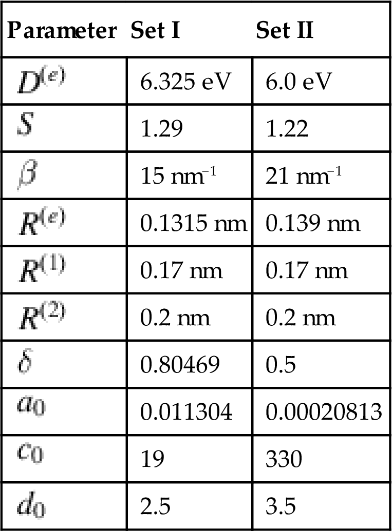
![]() in the aforementioned equations can be determined by fitting with the known physical properties of carbon. Brenner gave two sets of parameters, which are listed in Table 3.1 [33].
in the aforementioned equations can be determined by fitting with the known physical properties of carbon. Brenner gave two sets of parameters, which are listed in Table 3.1 [33].
Table 3.1
Brenner Potential Parameters of Sets I and II [33]
| Parameter | Set I | Set II |
| 6.325 eV | 6.0 eV | |
| 1.29 | 1.22 | |
| 15 nm−1 | 21 nm−1 | |
| 0.1315 nm | 0.139 nm | |
| 0.17 nm | 0.17 nm | |
| 0.2 nm | 0.2 nm | |
| 0.80469 | 0.5 | |
| 0.011304 | 0.00020813 | |
| 19 | 330 | |
| 2.5 | 3.5 |
Recently, a further revision of Brenner potential [37] called the second-generation reactive empirical bond order (REBO) potential, which is able to describe exactly the bonding structure and properties of graphite, diamond, and hydrocarbon molecules, is provided. In comparison with the Brenner potential, the second-generation potential includes both improved analytic functions for the interatomic interactions and an extended fitting database, which results in a significantly better description of the bond length, energies, and force constants for hydrocarbon molecules and elastic properties, interstitial defect energies, and surface energy for diamonds.
The REBO potential is also expressed as Eq. (3.2). To tell the second-generation potential from Brenner potential, superscript symbols are used, such as ![]() and
and ![]() are expressed as the pair term of repulsive and attractive potential
are expressed as the pair term of repulsive and attractive potential
(3.9)
(3.10)
where ![]() is the effective charge in the screened coulomb potential, and
is the effective charge in the screened coulomb potential, and ![]() limits the range of the covalent interactions and is given by
limits the range of the covalent interactions and is given by
(3.11)
 (3.11)
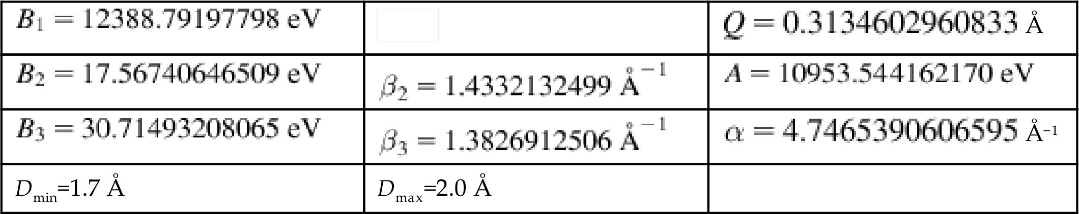
where ![]() is the distance over which the function goes from one to zero. The parameters obtained through data-fitting [37] are listed in Table 3.2.
is the distance over which the function goes from one to zero. The parameters obtained through data-fitting [37] are listed in Table 3.2.
The bond-order function between atoms i and j is given by
(3.12)
where the functions ![]() and
and ![]() depend on the local coordination and bond angles for atoms i and j, respectively. The function
depend on the local coordination and bond angles for atoms i and j, respectively. The function ![]() can be written as
can be written as
(3.13)
The first term ![]() in Eq. (3.13) depends on whether the bond has a radical character and is part of the conjugated system. The second term
in Eq. (3.13) depends on whether the bond has a radical character and is part of the conjugated system. The second term ![]() depends on the torsion angle for the C–C bonds. For bonds that are not part of the conjugated system, and for planar double bonds, both terms are equal to zero. The term
depends on the torsion angle for the C–C bonds. For bonds that are not part of the conjugated system, and for planar double bonds, both terms are equal to zero. The term ![]() in Eq. (3.12) is given as
in Eq. (3.12) is given as
(3.14)
An identical expression is given for ![]() by wrapping the i and j indices. The angle function
by wrapping the i and j indices. The angle function ![]() modulates the contribution that each nearest neighbor makes to the empirical bond-order according to the cosine of the angle of the bonds between atoms i and k, and i and j. To allow for both overcoordinated and undercoordinated atoms, a second spline function
modulates the contribution that each nearest neighbor makes to the empirical bond-order according to the cosine of the angle of the bonds between atoms i and k, and i and j. To allow for both overcoordinated and undercoordinated atoms, a second spline function ![]() was determined for angles less than
was determined for angles less than ![]() degrees that was coupled to the original angular function
degrees that was coupled to the original angular function ![]() . The term
. The term ![]() in Eq. (3.13) represents the influence of radical energies and the
in Eq. (3.13) represents the influence of radical energies and the ![]() bond conjugation on the bond energies. It accurately describes radical structures and accounts for nonlocal conjugation effects such as those governing the different properties of the C–C bonds in graphite. It is taken as a tricubic spline. The detail on the term
bond conjugation on the bond energies. It accurately describes radical structures and accounts for nonlocal conjugation effects such as those governing the different properties of the C–C bonds in graphite. It is taken as a tricubic spline. The detail on the term ![]() that describes the torsion angle for the C–C bonds can be found in [37].
that describes the torsion angle for the C–C bonds can be found in [37].
As mentioned above, the modified second-generation Brenner potential allows for covalent bond breaking and forming. Zhang et al. [38] adopted the modified second-generation Brenner potential to study the fracture of defected CNTs by atomistic and multiscale simulations. However, their numerical results revealed that the fracture stresses predicted by the second-generation Brenner potential is several times larger than those of quantum mechanics. This is due to the functional form of the cutoff function in the potential, which artificially magnifies the bond force for the distances between 1.7 and 2.0 Å and thus leads to a nonphysical failure mechanism. To overcome this problem, it is suggested [38,39] that this cutoff function be removed in the fracture analysis, but included in the C–C interactions only for those atom pairs that are less than 2.0 Å apart in the initial and undeformed configurations. Such an improvement makes the potential no longer able to handle bond formation, but it can provide accurate results for the fracture.
The short-range Brenner and REBO potentials do not model the nonbonding interactions between atoms. Hence, we computed the interspacing interaction between the SWCNTs in the bundles or multiwalled CNTs by using the long-range van der Waals potential which is described as
(3.15)
 (3.15)
where cn,k are cubic spline coefficients and ![]() =0.2 nm,
=0.2 nm, ![]() =0.32 nm, and
=0.32 nm, and ![]() =1.0 nm. EIJ is defined as the Lennard–Jones potential, which is computed as [40]
=1.0 nm. EIJ is defined as the Lennard–Jones potential, which is computed as [40]
(3.16)
where rij is the distance between atoms i and j, ![]() and
and ![]() . Eq. (3.16) reveals that the attenuation of the vdW interaction is quite rapid as the distance increases. It should be noted that our computational model will incorporate the van der Waals potential only if the covalent potential is zero, such that there is no artificial reaction barrier formed by the steep repulsive wall of the Lennard–Jones potential to prevent the nonbonded atoms from chemical reaction.
. Eq. (3.16) reveals that the attenuation of the vdW interaction is quite rapid as the distance increases. It should be noted that our computational model will incorporate the van der Waals potential only if the covalent potential is zero, such that there is no artificial reaction barrier formed by the steep repulsive wall of the Lennard–Jones potential to prevent the nonbonded atoms from chemical reaction.
Therefore, the total potential stored in the whole system is a sum of the short-range covalent and long-range noncovalent interactions
(3.17)
3.3 Elastic Properties of CNTs
3.3.1 Young’s Modulus of Single-Walled CNTs With Impurities
The system strain energy here is calculated using the REBO potential, and the Young’s modulus is obtained by applying the classical elasticity theory from
(3.18)
where the function E is the total strain energy of the system, ε is the strain, and V0 is the equilibrium volume.
3.3.1.1 Model of SWCNTs with impurities
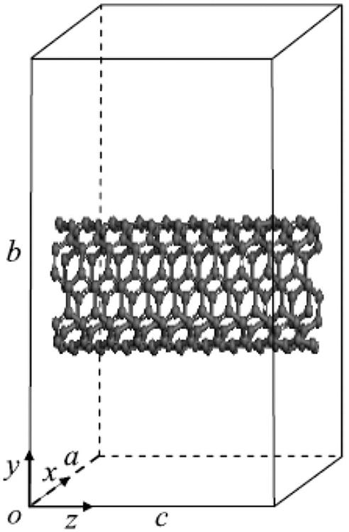
To construct armchair (5, 5) (10, 10) and zigzag (9, 0) (18, 0) SWCNTs, the atomic space coordinates in the basic unit are first determined. The structure of the SWCNTs can then be achieved by selecting carbon as the atom and coupling the bond properly. Similarly, the structure of BN-doped SWCNTs can be achieved by substituting a boron atom and a nitrogen atom for two adjacent carbon atoms. There is a deviation in the bond length due to the curvature effect of the tube wall. In general, it is found that the smaller the tube diameter, the greater the impact on the bond length. The initial bond lengths of the C–C, C–N, and C–B tubes are set to 1.42 Å, and the bond lengths of the B–N tubes are set to 1.45 Å. The calculated models are shown in Fig. 3.1, where Fig. 3.1C denotes a pure single-walled BNNT and Fig. 3.1D a pure SWCNT. The periodic structural units are then built by setting the basic unit of the SWCNTs in a cuboid crystal lattice; one end of the nanotubes is located at plane xy, and the other end is located on the opposite side plane, the axes of which are parallel to the crystal lattice axis z and pass the two centers of the planes that are face to face. To minimize the impact between CNTs, the lattice parameters, which are much larger than the diameter of the nanotubes, are set to a=b=100×10−10 m, as shown in Fig. 3.2. Finally, the structure is optimized, the electron density distribution is determined by using density functional theory (DFT), and the elastic parameters are computed using the MD method.

3.3.1.2 Effect of impurities on single-walled CNTs
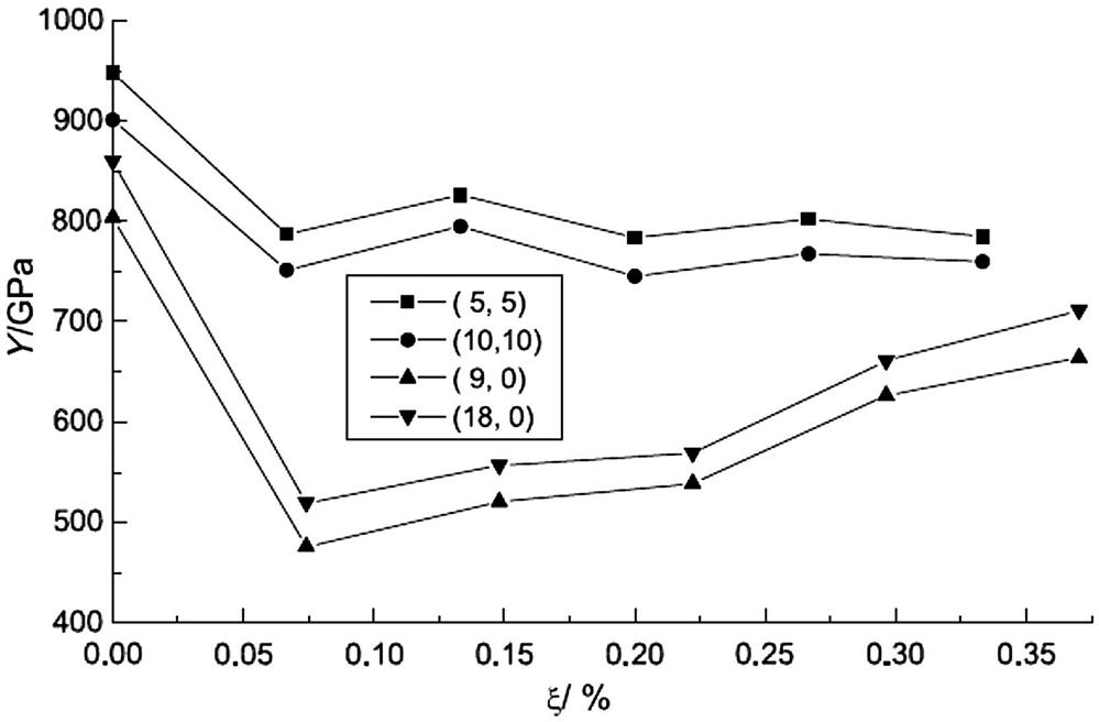
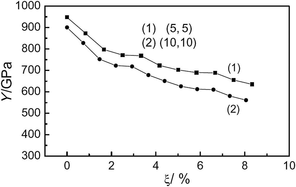
Fig. 3.3 shows the effect of various percentages of BN impurity (ξ) on the Young’s modulus (Y) of armchair (5, 5) (10, 10) and zigzag (9, 0) (18, 0) SWCNTs. The results indicate that the Young’s modulus of SWCNTs is generally very large, with the values for the armchair (5, 5) (10, 10) and zigzag (9, 0) (18, 0) SWCNTs without impurities being 948, 901 and 804, 860 GPa, respectively [41]. The Young’s modulus of the (5, 5) SWCNTs is very close to the value of 0.971 TPa reported in [42]. When the ratio of BN impurity in the armchair (5, 5) (10, 10) SWCNTs is about 6.7%, the Young’s modulus decreases by about 17%. However, further increases in the doping ratio do not cause the modulus to reduce further: it remains at about 800 and 760 GPa, respectively. The behavior of the zigzag SWCNTs is different. When the impurity ratio is about 7.5%, the Young’s modulus decreases by about 40%, but rises with further increases in the doping ratio. When the impurity ratio is 37%, the Young’s modulus decreases by only 17%. When the impurity ratio reaches 100% (i.e., boron–nitride nanotubes are formed), the Young’s modulus is 780 and 835 GPa, which is 97% of that of the corresponding pure SWCNTs (these values are not shown in Fig. 3.3).
3.3.1.3 Analysis of the results
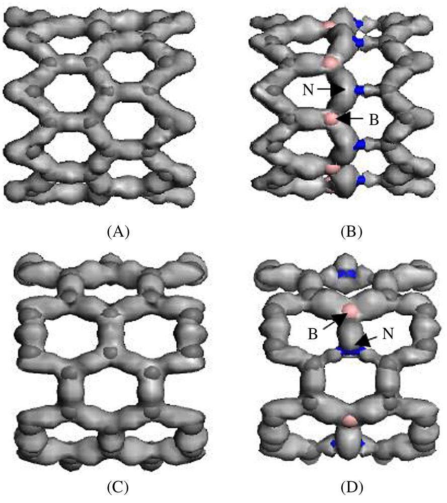
Because the effects of the different BN impurity ratios on the Young’s modulus of the same types of SWCNTs are similar, only (5, 5) was chosen from among the armchair SWCNTs and (9, 0) from among the zigzag SWCNTs to analyze the effects of BN doping on the electron density of SWCNTs. The comparison of the deformation electron density of SWCNTs with BN impurity and no impurity, which was derived using the local density approximation, is shown in Fig. 3.4.
Molecular orbitals are formed by an atomic orbital wave function through linear combination. Several atomic orbitals can be combined into several molecular orbitals. Half of the molecular orbitals are formed by two atomic orbitals with the same positive and negative symbols. The electronic probability density between the two nuclei increases, and the atomic energy becomes lower than the original atomic orbital energy. This is conducive to bonding and results in bonding molecular orbitals, such as the σ or π orbits. The other half of the molecular orbitals is formed by two atomic orbitals with different positive and negative symbols. The electronic probability density between the two nuclei decreases, and the atomic energy becomes higher than the original atomic orbital energy. This is not conducive to bonding, and thus these orbitals are known as antibonding molecular orbitals, such as the σ* or π* orbits. The π or π* bonds in CNTs are considered to be a hybridization of π or π* orbit bonding, which occurs in nanotubes when the π bond on the graphite layer degenerates into a large π bond on the carbon ring. Through the interaction and overlapping of adjacent large π bonds, a hybridization of the π bond and π* bond is formed.
As shown in Fig. 3.4, it is clear that atom B reveals more, atom C is less exposed, and atom N has been inundated in an electronic cloud. Therefore, compared with atom C, atom N can obtain electrons from atom B more easily. It can also be seen that when BN impurity is distributed around the circumference of the nanotubes, the existence of each N or B atom mostly affects the one bond in the axial direction in the zigzag SWCNTs, but also, to a lesser extent, affects the two bonds in the nonaxial direction in the armchair SWCNTs. This indicates that in the presence of BN doping, the Young’s modulus of zigzag SWCNTs decreases more than that of armchair SWCNTs. This phenomenon can be attributed to the change in the π orbital electron cloud that occurs when the π orbits bonded in the axial direction turn into antibonding π* orbits, which decreases the electron transfer in the circumferential direction. When the ratio of BN impurity in the SWCNTs increases, the increasing number of electrons in the circumferential direction improves the connectivity of zigzag SWCNTs, and strengthens the circumference direction σ bond. However, because the circumferential electron cloud of armchair SWCNTs is not connective, the increasing electron cloud in the circumferential direction does not strengthen the circumferential σ bond. Generally speaking, the σ bond and π bond in CNTs are related to their mechanical and electric properties, respectively. Therefore, the Young’s modulus of zigzag SWCNTs obviously increases with the percentage of BN impurity, whereas that of armchair SWCNTs tends to remains unchanged. These results concur with those shown in Fig. 3.3.
In performing data analysis on the Mulliken charges of SWCNTs doped with BN, it is find that the charge transfers only a little between B and C, but relatively more between B–N and N–C. For instance, in SWCNTs doped with 37% of BN, a 0.07e charge is transferred from B to C between B and C, a 0.17N charge is transferred from C to N between N and C, and a 0.55e charge is transferred from B to N between B and N. This means that each N obtains 0.72e and each B loses 0.62e. There are also small charge transfers among other atoms. This is caused by electronegativity: N>C>B, but the electronegativity within atom C is the same.
In BN-doped SWCNTs, polarity covalent bonds are formed in C–N and C–B, an electrovalent bond is formed in B–N, and a covalent bond is formed in C–C. Generally speaking, a mixed sp2 and sp3 covalent bond is formed in C–C close to N or B, and the other bonds are sp2 covalent bonds. The electron state distribution in BN-doped SWCNTs is thus relatively intricate. The cross-sections (A, B) and axial sections (C, D) of the electron density distribution of (5, 5), (9, 0) SWCNTs and the corresponding BN-doped SWCNTs are shown in Figs. 3.5 and 3.6, respectively. In these figures, (A), (C) show the electron distributing isosurface shape, and (B), (D) show the section isoline structure. The left, middle, and right figures show the situation for no, partial, and full impurity at the circumference, respectively. The figures show that there are some differences in the atomic bonding properties of the different constructions. The electron density distribution changes greatly for the N atom in the B–N bond (Fig. 3.5B3), which means that approximate electrovalent bonds are formed. In the N–C bond, the electron density distribution migrates slightly to N (Fig. 3.5B2), which means that a polarity covalent bond with a higher binding energy is formed. The electron migration in the CB bond can be attributed to the antibonding π* orbits (see Fig. 3.5B2).
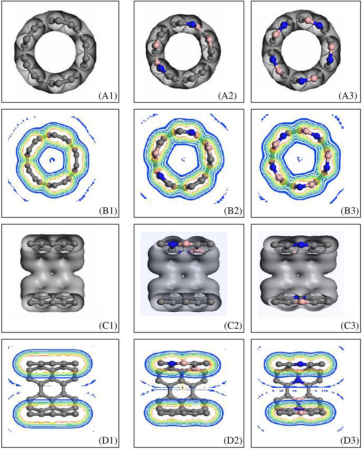
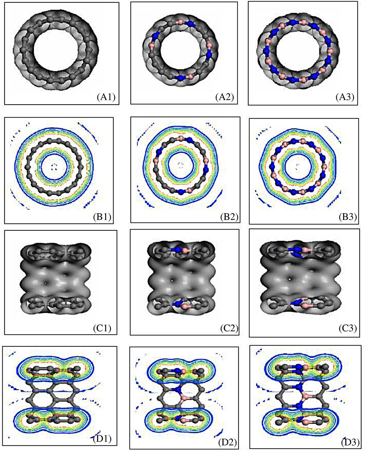
It is clearly shown in (B1) of Figs. 3.5 and 3.6 that because the electron density distribution among the C atoms overlaps, the symmetrical large ring orbits appear both inside and outside of the carbon ring. Parts (B2) and (B3) of the figures show that the electronic localization difference between B and N causes the distortion of the large ring orbits, especially for the lining orbits. Comparing Fig. 3.5D1 and Fig. 3.6D2, it can be observed that in the axial direction, the electric electron density distribution that results from the presence of large π bonds on the carbon ring in (5, 5) is clearly superior to that in (9, 0). Therefore, the electrical conductivity of the armchair nanotubes is better than that of the zigzag nanotubes in this direction. Figs. 3.5D2 and 3.6D2 show that the effects of BN impurity on the two types of nanotube are also different. The effects of BN on the inner and outer large ring orbits of (5, 5) are greater than the effects of the orbits in (9, 0) in these figures, whereas in Figs. 3.5B and 3.6B the effects of BN on (9, 0) are greater than those on (5, 5). These results indicate that the primary effect of BN impurity in armchair nanotubes occurs in the electron density distribution in the direction of the tube-axis, whereas in zigzag nanotubes it takes place in the circumferential direction. The results also indicate that the changes in the large π bond, which correlates with the electrical properties of nanotubes, also have an effect on their mechanical properties.
In CNTs, both the σ bond and the π bond can affect the Young’s modulus, but the contribution to the modulus originates mainly from the σ bond. Because the electron cloud of the σ bond overlaps more than that of the π bond, the local level of the σ bond is higher than that of the π bond. The electron density distribution on the outer orbit is relatively close to a line. Because of the structural characteristics of the armchair SWCNTs, the connectivity of the circumferential electron density distribution is relatively poor, and thus the mechanical properties mainly depend on the electron density distribution in the axial direction. As shown in Fig. 3.5D1–D3, the electron density distribution in SWCNTs undergoes an obvious change when the SWCNTs are doped with BN, but this change does not increase with increases in the impurity ratio. Fig. 3.6D1–D3 show that the electron density distribution in the direction of the tube-axis does not change greatly when the tube is doped with BN, but the electron density distribution in the circumferential direction does change in the presence of impurity, eventually reverting to the state without impurity. Therefore, when the impurity ratio is relatively low, the structural stability falls because of the difference in electronic localization between atoms B, N, and C. As the impurity ratio increases, the whole electron density distribution becomes more uniform and symmetrical, which compensates for the difference in electronic localization. It is known from previous analyses that the compensatory effect of zigzag SWCNTs is superior to that of armchair SWCNTs. In conclusion, when the ratio of BN impurity in armchair and zigzag SWCNTs is low, their Young’s modulus decreases. However, further increases in impurity do not give rise to a further decrease in the Young’s modulus. The modulus of the armchair SWCNTs remains at a certain value and fluctuates around it, whereas that of the zigzag SWCNTs increases with further increases in the impurity ratio. At the point at which pure boron–nitride nanotubes are formed, the Young’s modulus approaches that for pure SWCNTs.
3.3.2 Effects of Vacancy Defect Reconstruction on the Elastic Properties of CNTs
It is nearly impossible to obtain perfect CNT samples. In the process of the growth of CNTs, a variety of structural defects inevitably occur, which can have a big impact on the mechanical properties of the CNTs. In some cases, even a small number of defects can fundamentally change the mechanical performance. So, it is of great practical significance to conduct systematic research into CNT defects. In recent years, there have been many reports of 5–77–5 and vacancy defects and other types of structural CNT defects [43–51]. However, most of the studies have concentrated on the impact of defects on the electrical properties of CNTs. How do structural defects affect their mechanical properties? At present, there are still few reports. Therefore, it is necessary to study the impact of defects on the mechanical properties of CNTs. A research has been conducted to help us to gain a more comprehensive understanding of the structure of good CNTs [52].
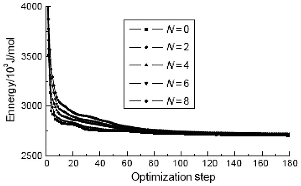
Vacancies are the most common defects in CNTs, and have drawn much research attention in recent years. Ajayan et al. [53] studied (10, 10) SWCNTs and confirmed that an ideal single vacancy containing three hanging bonds is unstable. He stated that two of the three dangling bonds tend to form a new C–C bond, and that the structure becomes a pentagonal ring coupled with one dangling bond, which forms a so-called 5–1DB defect. Lu and Pan [44] carried out a systematic calculation of single vacancies in SWCNTs and obtained the relationship between the vacancy formation energies and radii of different chiral SWCNTs. Krasheninnikov et al. [45] confirmed that vacancy defects are probable when using the Ar-ion process for low irradiation on (10, 10) SWCNTs, and stated that the process will be an instrument to control the structural defects of CNTs. In the early study of graphite structure, people found that there are usually two types of vacancies in graphite: single vacancy and di-vacancy [54]. As CNTs can be understood as curled graphite substrates, MD method is used to optimize these two kinds of initial structure defects at different temperatures and study the effect of different defect ratios on the Young’s moduli of SWCNTs. First, the reconstruction of single and di-vacancy structures in SWCNTs is optimized at different temperatures. Then, the Young’s moduli of SWCNTs with different single vacancy defect ratios are calculated. Finally, the results are analyzed according to the law of electron cloud coupling between the hanging bonds in the vacancies and the reconstruction features of the vacancy defects. Based on the analysis, the following conclusions can be derived. The reconstruction of vacancy defects can be carried out by way of not only temperature but also the defect ratios in SWCNTs because of the activity of dangling bonds and their space. Vacancy defects will bring about a decrease in the Young’s modulus, but their reconstruction will be an important factor in stabilizing the modulus. SWCNTs with vacancy defects can be energy suppliers by controlling vacancy reconstruction, which provides opportunities for designing new nanoelectromechanical system devices [55,56].
3.3.2.1 Model and methods
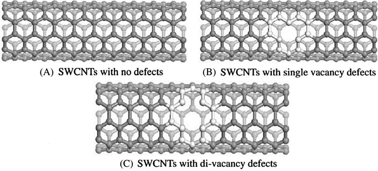
The atomic space coordinates are first calculated according to the construction of armchair (5, 5) and (10, 10) SWCNTs. The structure of the SWCNTs can then be achieved by selecting carbon as the atom and coupling the bond properly (as shown in Fig. 3.7A). The structure of single and di-vacancy defects can be achieved by removing one carbon atom and two adjacent carbon atoms, respectively, from the perfect SWCNTs (as shown in Fig. 3.7B and C). Periodic structural units are then built by setting the obtained SWCNTs in a cuboid crystal lattice. One end of the nanotube is located on plane xy and the other end is located on the opposite plane, the axes of which are parallel to the crystal lattice axis z and pass the two centers of the planes that are face to face. To minimize the impact between CNTs, the lattice parameters, which are much larger than the diameter of the nanotubes, are set to a=b=100×10−10 m. Finally, the structures are optimized at different temperatures, their electron density distribution is calculated using DFT, and the elastic parameters of SWCNTs with different single vacancy defect ratios are calculated using the MD method [52].
DFT is a quantum mechanical theory used in physics and chemistry to investigate the electronic structure of many-body systems, in particular atoms, molecules, and the condensed phases. DFT has been very popular for calculations in solid-state physics since the 1970s. In many cases, the results of DFT calculations for solid-state systems agreed quite satisfactorily with experimental data [57–59].
3.3.2.2 Vacancy defect reconstructions in single-walled CNTs
Fig. 3.8A and B are the optimized structures of (5, 5) single-walled CNTs with single and di-vacancy defects at different temperatures. The results indicate that when the temperature is below 2400K, the optimized single vacancy shows few changes, and there is no reconstruction. However, when the temperature is equal to or higher than 2400K, the optimized single vacancy shows obvious reconstruction. The structure becomes a pentagonal ring coupled with one dangling bond, which forms a so-called 5–1DB defect (Fig. 3.8A—2400K). The reconstruction of a di-vacancy is similar to that of a single vacancy. However, the di-vacancy has a higher reconstruction temperature and becomes an octagonal ring pinched into two pentagonal rings when the temperature is about or higher than 2600K. We call this structure a 5–8–5 defect (Fig. 3.8B—2600K). In Fig. 3.8, it is evident that the reconstruction configurations for single vacancy and di-vacancy remain unchanged when the temperature for (1) single vacancy is beyond 2500K and (2) di-vacancy is beyond 2700K. Therefore, the reconstruction configurations for them beyond these temperatures will not be presented.

In CNTs, the reconstruction of different types of vacancy defects takes place at different temperatures. The main reason is that when the vacancy defect is formed, it leads to a hanging bond around the vacancy (see the atoms with hanging bonds pointed by arrow in Fig. 3.8). If these dangling bonds need to be reformed into a new C–C bond, their activity must be enhanced to a certain extent. Temperature is a physical parameter that reflects the average kinetic energy of the microparticles: the higher is the temperature, the quicker are the microparticles and the greater is their average kinetic energy. Therefore, by increasing the temperature of the system, the electrons constituting a hanging bond can get more energy and the activity of the hanging bond will be enhanced. When the temperature is below a certain point, the activity of the hanging bond is below rebonding activity, so the transformation by optimizing the structure is very small, and no reconstruction happens. How single vacancies and di-vacancies are reconstructed and the temperatures required for the reconstruction primarily depend on the distance between the hanging bonds and surrounding environment. In general, the smaller the distance between the hanging bonds and the freer the electrons composing the hanging bonds, the lower the temperature necessary for reconstruction is. Thus, it can be seen from Fig. 3.8 that the single vacancy is easily reconstituted into a 5–1DB defect and the di-vacancy into a 5–8–5 defect. The reconstitution temperature of the di-vacancy is higher than that of the single vacancy, as the new 5–8–5 structure does not have a hanging bond; its acquired energy is required for four hanging bonds, close to two 5–1DB defects. Of course, the reconstitution temperature of di-vacancy defects also depends on the diameters of tube and orientation of the defects. It can be forecasted that because of the curvature of the tube wall, either different diameters or a different orientation will lead to small changes in the distance between the hanging bonds and greater changes in the reconstitution temperature. In addition, the reconstruction of the defects can further release the potential energy of the system to make the structure more compact, which helps to improve the stability of the structure. Fig. 3.9 presents the optimization energy curves of the aforementioned structures. When the temperature is less than that required for reconstruction, it can be seen from the figure that the optimized single and di-vacancy structures have different stable potential energies, and that despite the temperature increase, the potential energies remain unchanged. These are −1319.6 and −1309.9 eV, respectively. The potential energy of the di-vacancy is higher than that of the single vacancy when the number of hanging bonds in the di-vacancy is greater. When the temperature reaches the degree necessary for reconstruction, the potential energies at stability for the single and di-vacancy structures fall suddenly to −1321.2 and −1313.5 eV, respectively, which indicates that reconstruction happens, energy is released, and the structure becomes more stable. From the point of view of quantum mechanics, there is a barrier between the vacancy states before and after reconstruction. Only when the hanging bonds get sufficient energy can they overcome the barrier and bond to form a more stable structure. The higher reconstitution temperature for the di-vacancy compared to that for the single vacancy indicates that its barrier is higher. Using the reconstitution temperature (T) and the potential energy before and after reconstruction (Ep1, Ep2), the following results can be calculated: vacancy barrier ![]() (where the Boltzmann constant
(where the Boltzmann constant ![]() =1.38×10⁻²³ J/K), the potential energy difference between the pre- and postreconstruction stages
=1.38×10⁻²³ J/K), the potential energy difference between the pre- and postreconstruction stages ![]() , and the releasable energy in the process of the reconstruction
, and the releasable energy in the process of the reconstruction ![]() . The results are shown in Table 3.3. The greater decline in potential energy indicates that di-vacancy reconstruction greatly contributes to improving the stability of the structure.
. The results are shown in Table 3.3. The greater decline in potential energy indicates that di-vacancy reconstruction greatly contributes to improving the stability of the structure.
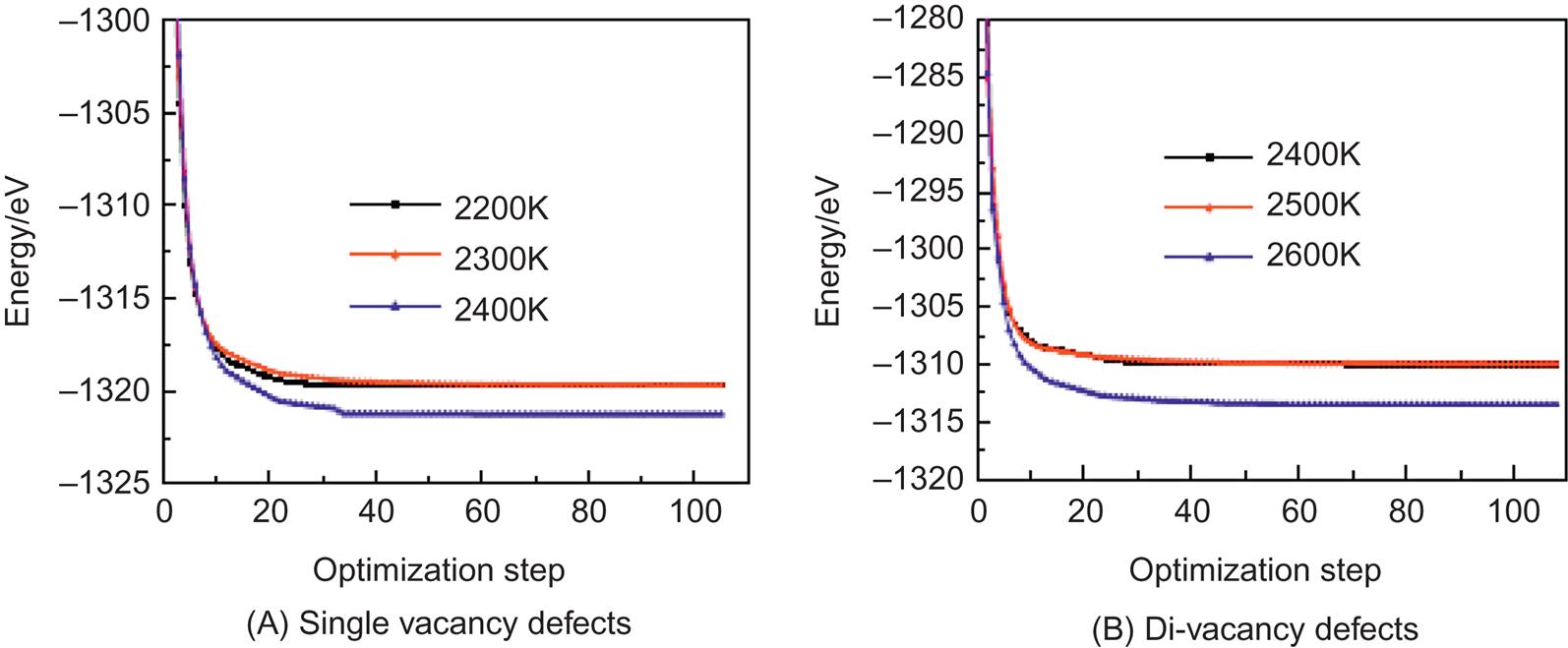
Table 3.3
Energy (eV) of (5, 5) SWCNTs With Vacancy Defects [52]
| Type of Vacancy | T (K) | |||||
| Single vacancy | 2400 | −1319.6 | −1309.9 | 0.207 | 1.6 | 1.807 |
| Di-vacancy | 2600 | −1321.2 | −1313.5 | 0.224 | 3.6 | 3.824 |
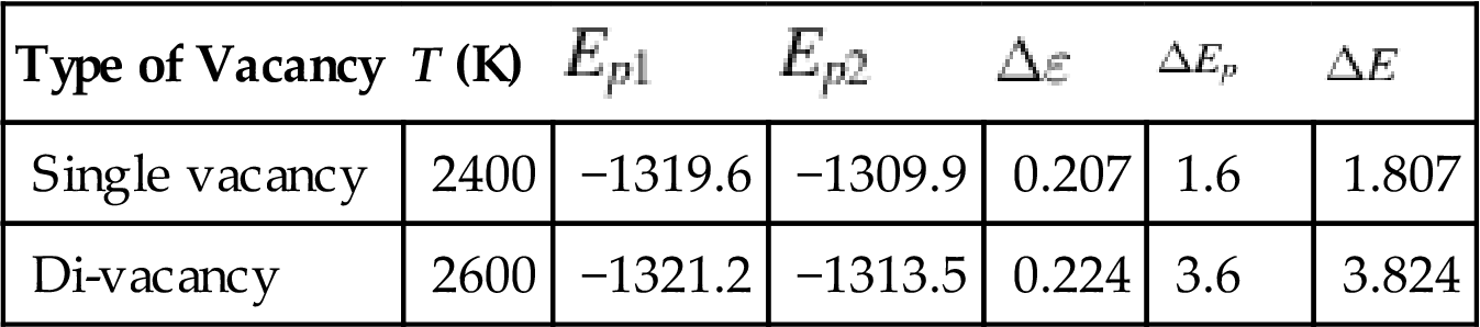
Fig. 3.10 shows the deformation electron densities and their isolines on sections of CNTs with single and di-vacancy defects before and after reconstruction. Therein, the left figures (Fig. 3.10a(A) and b(B)) represent the distribution of deformation electron densities, and the middle and right figures represent the distribution of their cross-section and axial section isolines, respectively. The electron density is the same as the online equivalent, and the deformation electron density gradually becomes smaller on the vertical isolines from the inside outward. The isoline intervals reflect the local electronic conditions, in that the greater is the interval, the weaker is the localization and the freer the electrons, and vice versa. By comparing Fig. 3.10a1 and b1, it is clear that a new bond has formed between two dangling bonds in the nonaxial direction, and that the electron density distribution composing the bond is close to that of other C–C bonds of nondefective CNTs. This indicates the formation of a new C–C bond. However, the situation for Fig. 3.10A1 and A2 is somewhat different, as the formation of new C–C bonds takes place between two pairs of axial dangling bonds. Comparing Fig. 3.10a2(A2) and b2(B2), the electrons of the atomic outer layers around the defects on the cross-section transfer to the defects after the reconstruction, and the distribution of the electron density takes on a connecting trend. From Fig. 3.10a3(A3) and b3(B3), we can also see that the axial section resembles the transition circumstances of the cross-section, with narrowing of the electron density center making the spatial distribution region uniform and improving the stability of the structure. In particular, the di-vacancy makes a relatively great contribution in the axial direction.
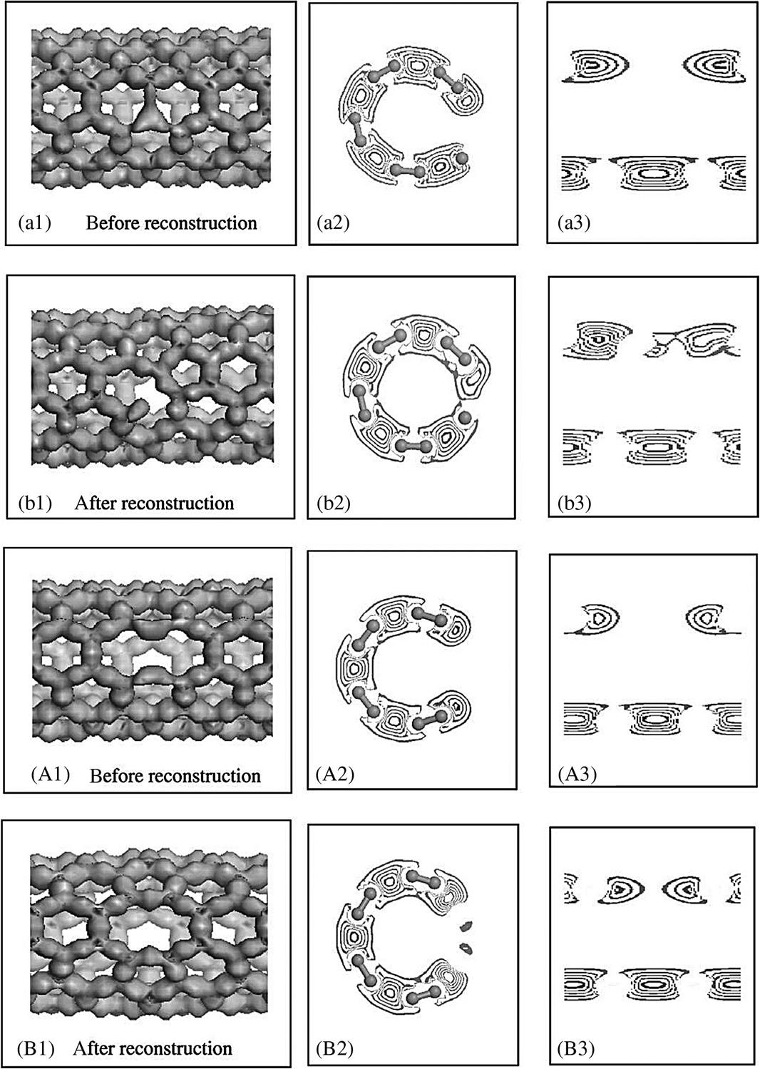
Molecular orbitals are formed by an atomic orbital wave function through a linear combination. Several atomic orbitals can be combined into several molecular orbitals. Half of a molecular orbital is formed by two atomic orbitals with the same positive and negative symbols. The electronic probability density between the two nuclei increases, and the atomic energy becomes lower than the original atomic orbital energy. This is conducive to bonding and results in bonding molecular orbitals, such as the σ or π orbits. The other half of a molecular orbital is formed by two atomic orbitals with different positive and negative symbols. The electronic probability density between the two nuclei decreases, and the atomic energy becomes higher than the original atomic orbital energy. This is not conducive to bonding, and thus these kinds of orbitals are known as antibonding molecular orbitals such as the σ* or π* orbits. The CNTs under study are composed of a number of carbon hexagonal rings, and their structure can thus be considered to be a rolled-up graphene sheet in which the localized strong σ bond and delocalized π bond are formed by combining each carbon atom with the three adjacent carbon atoms through sp2 hybrid orbital bonding. The σ and π bonds are located, respectively on and perpendicular to the tube wall. The transformation of vacancy defects in CNTs can be understood as follows. Because of the vacancy, class π bonds near the defects on the tube wall are destroyed, creating much local stress at the defects. The formation of new C–C bonds can effectively eliminate part of the stress, resulting in the spontaneous transformation of the vacancy into a 5–1DB or 5–8–5 defect.
From Fig. 3.10a1, we can see the electronic distribution that appears among the three hanging bonds; however, the electrons are little bound by their C atomic kernel, their energy is great, the mid-density between the two nuclei is small, and the bonds are weak. This indicates that σ* or π* bonds that are related to conductivity are mainly taken on. Comparing Fig. 3.10a3 and b3, we can see that the isoline interval around the defects becomes denser after reconstruction. Therefore, after reconstruction, the partial σ* or π* bonds have primarily been transformed into σ or π bonds, which make a larger contribution to the elasticity. From Fig. 3.10B1 (compared with Fig. 3.10A1), we find that some axial C atoms near the defect are more revealed, and that other C atoms are less exposed or are inundated in an electronic cloud. This is because partial electrons recombined to form new C–C bonds come from the transfer of axial p electrons that form π bonds. There are two recombined bonds in a 5–8–5 defect and only one in a 5–1DB defect, and thus more electrons are required in the 5–8–5 defect.
3.3.2.3 Effect of single vacancy defect ratio on Young’s modulus of single-walled CNTs
Fig. 3.11 shows the effect of various percentages of vacancy defects (ξ) on the Young’s modulus (Y) of armchair (5, 5) and (10, 10) SWCNTs at 298 K. The results indicate that the Young’s modulus of SWCNTs is generally very large, with the values for the armchair (5, 5) and (10, 10) SWCNTs with no defects being 948 and 901 GPa, respectively, at room temperature. The Young’s modulus of the (5, 5) SWCNTs is very close to the value of 0.971 TPa reported in [42]. With an increase in the single vacancy defect ratio in SWCNTs, the Young’s moduli will decrease. However, when the vacancy defect achieves a certain ratio, such as ξ=2.5% and ξ=5.83% for (5, 5) and ξ=2.2% and ξ=5.86% for (10, 10) SWCNTs, there is a sudden slowdown in the curves of the Young’s moduli versus the vacancy defect radio and the platform phenomenon emerges.
A vacancy will result in hanging bonds near the carbon atoms and a relaxed structure, leading ultimately to a decrease in the elastic moduli. The platform phenomenon in this decrease means that the influence of the defects on the system structure will be reduced, and the elasticity of the system will become stable for the following two reasons. First, normally, when the vacancy rate is smaller, mainly single vacancies are present in the system, and di-vacancies seldom appear. In contrast, when the rate becomes larger, the space between two adjacent single vacancy defects will become smaller. When the space is reduced to zero (namely, a di-vacancy), the boundaries of the defects will be partly superimposed, which leads to a great reduction in the number of hanging bonds. From the structural characteristics of the defects, we know that two single vacancies produce six hanging bonds, whereas one di-vacancy produces only four hanging bonds. Therefore, when the defect rate is small, compared with the influence of the two separate single vacancies, that of the di-vacancy on the CNT is smaller. However, the main reason that the system elasticity tends to become stable should be that reconstruction has taken place in some of the vacancies. In the abovementioned investigation, we consider only the impact of temperature on the reconstruction of one defect in a CNT. However, for CNTs that have a higher vacancy rate, the reconstruction of defects still occurs. When the vacancy rate increases gradually, the distance between the defects decreases naturally, and most of the hanging bonds are created. When the distance is narrowed to a certain pitch, the bonds can easily interact with each other. The activity of the large number of hanging bonds should follow a distribution similar to Maxwell speed distribution in thermodynamics. As a result, even at a temperature lower than the reconstruction temperature required for single vacancy defects, when the defects reach a certain percentage, there are always some highly active hanging bonds, and some of them are neighbors, so then the bonds will combine with each other to form 5–1DB or 5–8–5 defects. Then, the energy of the system will begin to be released, and the released energy can also activate more hanging bonds with lower activity to allow reconstruction to take place continuously within a certain range. In this way, the structure will be stable for the time being, which results in a sudden delay in the decline of the Young’s moduli, and subsequently, the plateau effect. In addition, the energy brought by the reconstruction is enough to activate the hanging bond with lower activity to bond (see Table 3.3, ![]() ), and a source releasing energy can be generated by controlling the temperature at a location. The activation effect spreads further, from the near to the distant vacancy, creating a new reconstruction and releasing energy continuously. As a result, the magnitude and continuous time releasing energy can be adjusted by the defect rate, and the defect rate can be controlled by using the Ar-ion process for low irradiation on SWCNTs [60]. Therefore, an SWCNT with vacancy defects is expected to be an energy supplier by controlling vacancy reconstruction.
), and a source releasing energy can be generated by controlling the temperature at a location. The activation effect spreads further, from the near to the distant vacancy, creating a new reconstruction and releasing energy continuously. As a result, the magnitude and continuous time releasing energy can be adjusted by the defect rate, and the defect rate can be controlled by using the Ar-ion process for low irradiation on SWCNTs [60]. Therefore, an SWCNT with vacancy defects is expected to be an energy supplier by controlling vacancy reconstruction.
3.3.3 Young’s Moduli of Single-Walled CNTs With Grafts
3.3.3.1 Model of SWCNTs with grafts
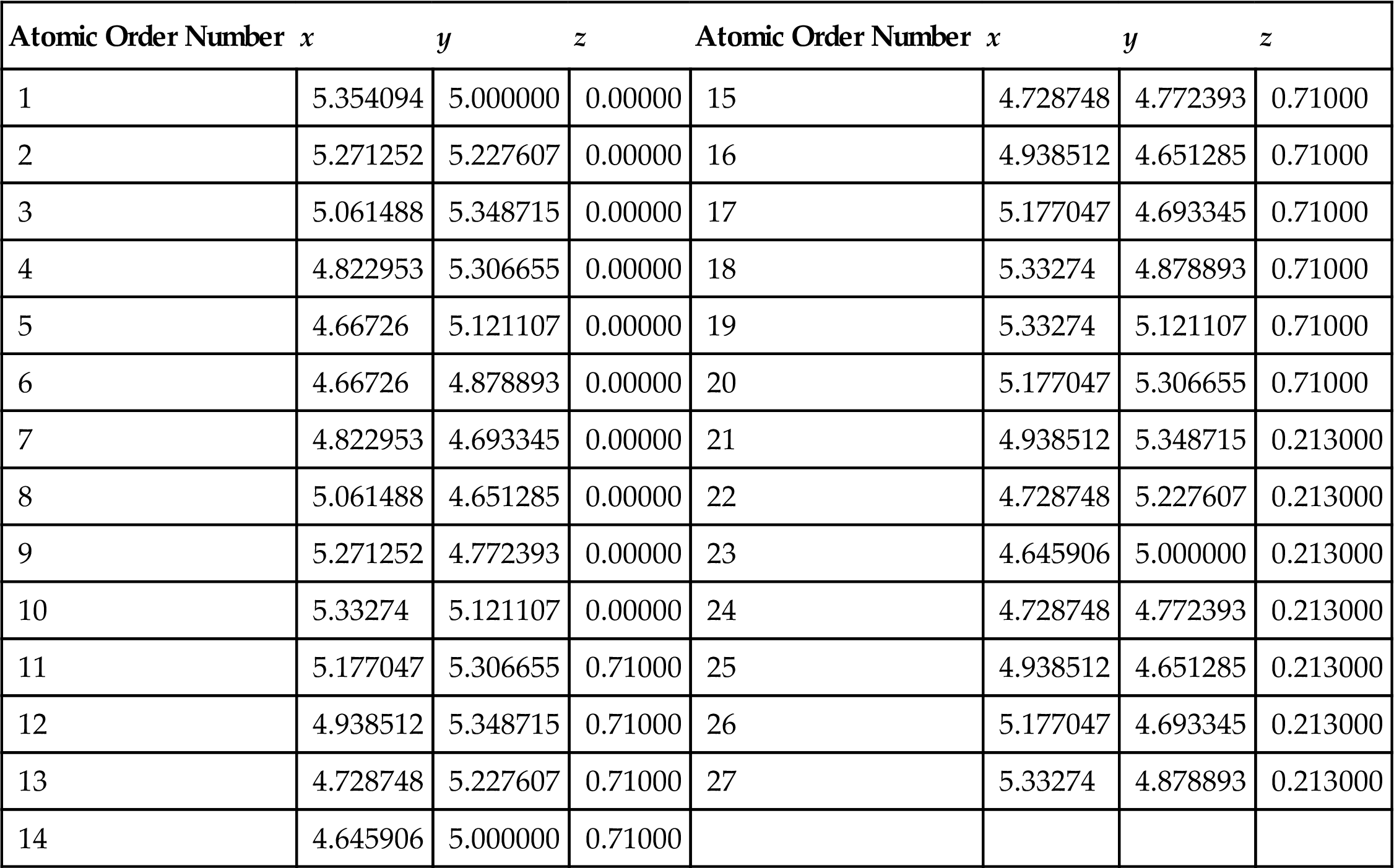
As shown in Fig. 3.2, the atomic space coordinates in the basic unit are first calculated according to the construction of the armchair (5, 5) (10, 10) and zigzag (9, 0) (18, 0) SWCNTs (see Tables 3.4 and 3.5). The structure of the SWCNTs can then be achieved by selecting carbon as the atom and coupling the bond properly. Usually, there are two basic types of CNT ends: open and closed. Open-ended CNTs are considered to be more active, and are often selected to practically enhance composite materials. Therefore, open-ended CNTs are considered here, and 2–8 amine functional groups are linked symmetrically at both ends of the CNTs. In Fig. 3.12, the functional group atom marked with an arrow is grafted to a carbon atom at one end such that the C–C bonds at the grafts are parallel to the tube axes of the CNTs. The calculated model is shown in Fig. 3.12. The DMol3 software is used to optimize the structure and calculate the related electric properties. The periodic structural units are then built by setting the basic unit of the SWCNTs in a cuboid crystal lattice. One end of the nanotubes is located on plane xy and the other end is located on the opposite plane, the axes of which are parallel to the crystal lattice axis z and pass the two centers of the planes, which are face to face. To minimize the impact between the CNTs, the lattice parameters, which are much larger than the diameter of the nanotubes, are set to a=b=100×10−10 m, as shown in Fig. 3.2. Once the structure is optimized, the electron density distribution is calculated by using the DFT. Then, the amine functional groups are cut off from the optimized structures. Finally, the elastic parameters are calculated by using the MD method.
Table 3.4
Atom Coordinates (nm) in the Basic Cell of (5, 5) SWCNTs [66]
| Atomic Order Number | x | y | z | Atomic Order Number | x | y | z |
| 1 | 5.311295 | 5.138886 | 0.00000 | 11 | 5.170208 | 5.295335 | 0.122976 |
| 2 | 4.964107 | 5.338977 | 0.00000 | 12 | 4.771717 | 5.253141 | 0.122976 |
| 3 | 4.666522 | 5.070614 | 0.00000 | 13 | 4.688705 | 4.861114 | 0.122976 |
| 4 | 4.829792 | 4.704665 | 0.00000 | 14 | 5.035893 | 4.661023 | 0.122976 |
| 5 | 5.228283 | 4.746859 | 0.00000 | 15 | 5.333478 | 4.929386 | 0.122976 |
| 6 | 5.340872 | 5.000000 | 0.00000 | 16 | 5.275771 | 5.20036 | 0.122976 |
| 7 | 5.105335 | 5.324189 | 0.00000 | 17 | 4.894665 | 5.324189 | 0.122976 |
| 8 | 4.724229 | 5.200360 | 0.00000 | 18 | 4.659128 | 5.000000 | 0.122976 |
| 9 | 4.724229 | 4.799640 | 0.00000 | 19 | 4.894665 | 4.675811 | 0.122976 |
| 10 | 5.105335 | 4.675811 | 0.00000 | 20 | 5.275771 | 4.79964 | 0.122976 |
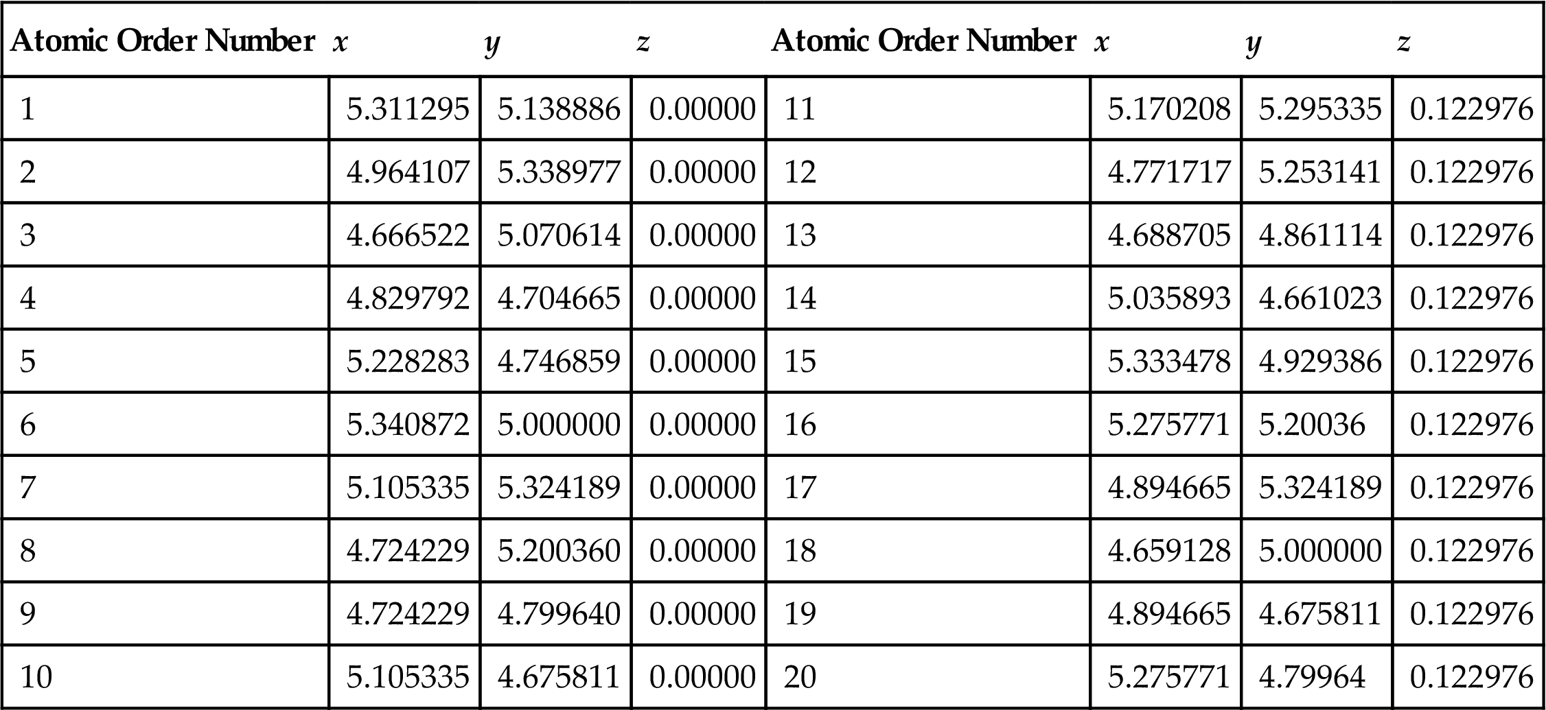
Table 3.5
Atom Coordinates (nm) in the Basic Cell of (9, 0) SWCNTs [66]
| Atomic Order Number | x | y | z | Atomic Order Number | x | y | z |
| 1 | 5.354094 | 5.000000 | 0.00000 | 15 | 4.728748 | 4.772393 | 0.71000 |
| 2 | 5.271252 | 5.227607 | 0.00000 | 16 | 4.938512 | 4.651285 | 0.71000 |
| 3 | 5.061488 | 5.348715 | 0.00000 | 17 | 5.177047 | 4.693345 | 0.71000 |
| 4 | 4.822953 | 5.306655 | 0.00000 | 18 | 5.33274 | 4.878893 | 0.71000 |
| 5 | 4.66726 | 5.121107 | 0.00000 | 19 | 5.33274 | 5.121107 | 0.71000 |
| 6 | 4.66726 | 4.878893 | 0.00000 | 20 | 5.177047 | 5.306655 | 0.71000 |
| 7 | 4.822953 | 4.693345 | 0.00000 | 21 | 4.938512 | 5.348715 | 0.213000 |
| 8 | 5.061488 | 4.651285 | 0.00000 | 22 | 4.728748 | 5.227607 | 0.213000 |
| 9 | 5.271252 | 4.772393 | 0.00000 | 23 | 4.645906 | 5.000000 | 0.213000 |
| 10 | 5.33274 | 5.121107 | 0.00000 | 24 | 4.728748 | 4.772393 | 0.213000 |
| 11 | 5.177047 | 5.306655 | 0.71000 | 25 | 4.938512 | 4.651285 | 0.213000 |
| 12 | 4.938512 | 5.348715 | 0.71000 | 26 | 5.177047 | 4.693345 | 0.213000 |
| 13 | 4.728748 | 5.227607 | 0.71000 | 27 | 5.33274 | 4.878893 | 0.213000 |
| 14 | 4.645906 | 5.000000 | 0.71000 |

To accurately determine the Young’s modulus of CNT, its wall thickness of different diameters should take on different values, however, it was reported that the differences are generally very small [61–65]. In this study, the effects of grafted amines on the CNT are studied where the CNT wall thickness of 0.34 nm is used in the simulation.
3.3.3.2 Effect of amine grafts on SWCNTs
Fig. 3.13 shows the effect of different numbers of grafted amines on the Young’s moduli of two hexagonal units of tube-length armchair (5, 5) (10, 10) and zigzag (9, 0) (18, 0) SWCNTs. The results indicate that the Young’s moduli of the SWCNTs are generally very large, with the values for the armchair (5, 5) (10, 10) and zigzag (9, 0) (18, 0) SWCNTs without grafts being 948, 901 and 804, 860 GPa, respectively [66]. The Young’s moduli of the (5, 5) SWCNTs are very close to the value of 0.94 TPa reported in [64]. In general, the effect of tube length on the Young’s modulus of CNT is small. For the comparison purposes, the CNTs in this study are all set in the same cuboids crystal lattice (see Fig. 3.2), i.e., the CNTs are of infinite lengths. It was found that the effect of tube diameter on the elastic properties of CNT are size-dependent [65,67], but the Young’s modulus of CNT is not a monotone continuous variation with the tube diameter [68]. It is known that the armchair CNT and zigzag CNT are different in their structure. Their basic hexagon units are perpendicular to each other; therefore, the size-dependent Young’s modulus should be different. It was reported that the Young’s modulus increases with the decrease of the tube radius [69,70]; but opposite trends were also reported [65]. It indicates that a further investigation of the Young’s modulus is worth carrying out.

When the zigzag SWCNTs are grafted with amine, their Young’s moduli decrease slightly, but an increase in the graft number does not cause any further reductions in the moduli, which basically remain at about 95% of those of the zigzag SWCNTs without grafts. The armchair SWCNTs behave somewhat differently when grafted with amine, with a marked drop in the Young’s moduli. When the graft number is 2 or 4, the Young’s moduli drop by 17% and 26%, respectively, but the decrease then slows until the moduli remain at a certain value with further increases in the graft number. When the graft number reaches 6 or 8, the Young’s moduli are about 72% of those of the armchair SWCNTs without grafts.
SWCNTs can be classified as zigzag, armchair, or chiral types according to their chiral angle. The chiral angle of zigzag nanotubes is 0 degree, whereas that of armchair nanotubes is 30 degrees. The chiral angle of chiral SWCNTs is greater than 0 degree and less than 30 degrees. Therefore, the foregoing results indicate that the effects of amine grafts on the elastic properties of SWCNTs are related to their chiral angle.
3.3.3.3 Analysis of the results
As the effects of amine grafting on the elastic modulus follow a similar law for the same types of CNTs, only (5, 5) and (9, 0) CNTs are selected for analysis. Figs. 3.14 and 3.15 show the deformation of the electronic distribution and density sections of the isolines as calculated by DFT theory by simulating (5, 5) and (9, 0) SWCNTs in a 0 to 8–graft model. The electron density is same as the online equivalent, and the deformation of the electron density gradually becomes smaller on the vertical isolines from the inside outward. The isoline intervals reflect the local electronic conditions, in that the greater the interval, the weaker the localization and the freer the electrons, and vice versa.
As shown in Fig. 3.14, when the armchair SWCNTs are grafted, the outer electron density of the CNTs decreases and their inner isoline interval become obviously denser as the number of grafts increases, which indicates an increase in the localization of the s electron. The inner s electronic isoline interval tends to remain stable, which shows that the electronic shackles from the atomic nucleus become stabilized to some extent when enhanced. The outer-layer electrons are the main cause of the covalent bond. The stronger the shackles of the nucleus on the s electron, the less likely the possibility of electronic stimulation from 2s to 2p. Consequently, the sp hybrid probability declines and the outer-layer electrons and number of bonds decrease, which results in structural stability and a decline in the elastic modulus. At the same time, it is observed for 1–4 amines that the nonlocalized outer large π bond electrons gradually flow to the grafting area at the ends of the nanotubes. This indicates that both the conductivity and the bonding electrons, which maintain the stability of the structure, have decreased. The resulting elastic moduli reflect a decline in structural stability. As the number of grafts increases further, the electron density tends toward a stable state and the elastic moduli remain the same. However, the situation for the zigzag SWCNTs is different. It can be seen from Fig. 3.15, which describes the zigzag SWCNTs, that both the electron density of the nonlocalized outer layer of the large π bond, which is related to the conductivity, and the electron density of the r bond within the domain change little as the quantity of grafts changes. The isoline intervals also show no obvious change when the graft quantity changes. Fig. 3.14 and 3.15 show that the deformation electron density follows a similar change law to the elastic modulus (Fig. 3.13).
As shown in Tables 3.6 and 3.7, the C–C bond length of the SWCNTs changes as a result of grafting. The C–C covalent bond length is closely related to s and p components in the hybrid orbital. The reduction of the p component and the increase of the s component result in a shortening of the bond length. This is because the space configuration of the s orbital determines that its electronic cloud is close to the atomic nucleus and its orbital radius is smaller, and the space configuration of the p orbital determines that its electronic cloud is further away from the atomic nucleus and its orbital radius is larger. There are usually three hybrid forms of carbon atoms, namely, sp3, sp2, and sp. In a hybrid orbital, if the s component increases, then the orbital energy will be reduced and the effective radius decreased, and the covalent bond length will be shortened accordingly. The CNTs under study are composed of a number of carbon hexagon rings, and their structure can thus be considered as a rolled-up graphene sheet where the localized strong σ bond and delocalized π bond are formed by combining each carbon atom with the three adjacent carbon atoms through sp2 hybrid orbital bonding.
Table 3.6
The C–C Bond-Length (nm) of the Optimized (5, 5) Nanotubes With Grafts [66]
| Graft Number | Center | Port Circumferential Direction | ||
| Circumferential Direction | Axial Direction | Further from Graft | Nearer to Graft | |
| 0 | 0.1469 | 0.1468 | 0.1448 | 0.1448 |
| 2 | 0.1467 | 0.1482 | 0.1446 | 0.1567 |
| 4 | 0.1465 | 0.1493 | 0.1447 | 0.1570 |
| 6 | 0.1466 | 0.1497 | 0.1447 | 0.1572 |
| 8 | 0.1465 | 0.1497 | 0.1448 | 0.1573 |

Table 3.7
The C–C Bond-Length (nm) of the Optimized (9, 0) Nanotubes With Grafts [66]
| Graft Number | Center | Port Circumferential Direction | ||
| Circumferential Direction | Axial Direction | Further from Graft | Nearer to Graft | |
| 0 | 0.1443 | 0.1504 | 0.1405 | 0.1405 |
| 2 | 0.1442 | 0.1502 | 0.1406 | 0.1418 |
| 4 | 0.1442 | 0.1505 | 0.1407 | 0.1426 |
| 6 | 0.1444 | 0.1501 | 0.1408 | 0.1424 |
| 8 | 0.1443 | 0.1506 | 0.1411 | 0.1427 |
Tables 3.6 and 3.7 show that the C–C bond length in the center of the optimized zigzag (9, 0) SWCNTs changes little in the circumferential and axial directions when the graft number increases. This indicates that the stability of the structure does not change, and thus that the Young’s moduli undergo almost no change as the graft number increases. The armchair (5, 5) SWCNTs, in contrast, behave totally differently. When their ends are grafted with amines, the C–C bond-length in the center is shortened slightly in the circumferential direction, and the impact of the graft number on the bond length is small. In contrast, the C–C bond length in the axial direction is significantly elongated, and the impact of the graft number on the bond length is large. When the nanotubes are grafted with 0–4 amines, the bond length is elongated, but when the graft number reaches 6, the bond length basically remains unchanged. In general, the greater the bond-length difference in the circumferential and axial directions, the greater the decline in structural stability and the smaller the elastic modulus. This may be the main reason for the difference in the elastic moduli of the armchair and zigzag SWCNTs of the same tube diameter without grafts. It is clear from Tables 3.6 and 3.7 that the C–C bond-length changes in the grafted armchair SWCNTs are almost the same as the elastic modulus changes. The bond-length changes can be attributed to a certain number of p electron-bonding transfers. The p electrons in the center of the grafted armchair SWCNTs transfer from the circumferential direction to the axial direction and the grafted ends. This results in a reduction in the p component and an increase in the s component in the circumferential direction, and an increase in the p component and reduction in the s component in the axial direction in the bonding capacity of the hybrid orbital. In CNTs, the σ bond and π bond can be built by electron coupling in the outer layer of carbon atoms. Both the σ bond and the π bond can affect the Young’s modulus, but the main contribution comes from the σ bond. Because the stability of the σ bond is greater, it is impossible for its electron-bonding to undergo an obvious shift. The mobility of the π electron bond is greater, which is directly related to the conductivity. Consequently, electron transfers in the circumferential direction can be divided into two types. In the first type, p electrons form a σ bond that transfers in the axial direction to the nearest neighbor, but the transfer number has a saturation property. This means that when the number of grafts reaches 6, the number of p electrons in the axial direction no longer increases. In the second type, more p electrons form and the bond is transferred to the distant ports where the grafts are. In this case, the bond-length changes are not very large, and the shorter the bond length, the smaller the distance between the atoms and the greater the energy absorbed from the splitting of the covalent bond. Consequently, if the bond energy is high, then the bond is strongly stable and the elastic modulus is large. The elastic moduli of amine-grafted armchair SWCNTs thus depend primarily on the axial bond length in the center. The axial bond-length changes in the center of armchair SWCNTs with different numbers of amine grafts have a strong relation with the corresponding changes in the Young’s modulus.
To further analyze the impact of grafts on the Young’s moduli of SWCNTs, the total deformation potential energy of the optimized structure of SWCNTs with different numbers of grafts is calculated. The calculated results for (5, 5) and (9, 0) SWCNTs with 0–8 grafts at their ports are shown in Figs. 3.16 and 3.17. It can be seen that the potential energy is about 2710 kJ/mol after the structure of the (9, 0) SWCNTs has been optimized to a stable state, and that the value does not show any clear correlation with the graft number. The behavior of (5, 5) SWCNTs is rather different, with a stability potential energy value when no grafts are present of 2650 kJ/mol. This value rises to 2715 kJ/mol with a 2–amine graft and 2748 kJ/mol with a 4–amine graft, and then remains at about 2750 kJ/mol for any further increases in graft number. These changes basically concur with those shown in Fig. 3.13.
The total deformation potential energy of a molecular structure is calculated using an analytical function that is a sum of a number of individual energy terms. At its simplest level, this function includes bond stretching, valence angle bending, torsion, and nonbonded interaction terms, all of which determine the energetic penalty of the structure based upon deviations from idealized equilibrium geometry. For instance, the bond term is a summation of all of the bonds in the structure, in which the energy of each bond is evaluated based on how far it is deformed from its equilibrium value. The total deformation potential energy being different from the aforementioned optimized structures indicates that the deviations from the idealized equilibrium geometry are different. The deformation of a structure creates equilibrium space variety among its atoms. When the distance between a pair of atoms is greater, an attraction will appear between them. When the distance is small, the electronic cloud repulsion between the atoms will work quickly in accordance with Pauli’s exclusion principle. The equilibrium spacing between atoms near the origin equilibrium position is fixed by two opposite effects. According to linear elastic theory, the net force between the atoms is proportional to the deviations between the actual and idealized equilibrium spacing, and its potential role is proportional to the square of the deviations; the greater the structural deviations, the higher the potential energy. This suggests that the looser its intermolecular combining, the more easily the structure will be deformed and the smaller its Young’s modulus will be. The total deformation potential energy variabilities of the optimized armchair (5, 5) and zigzag (9, 0) SWCNTs with different graft numbers have a good relation with their corresponding Young’s modulus variations.
3.4 Structural Stability and Buckling of CNTs
3.4.1 Buckling of SWCNTs and MWCNTs
This study is to provide a comprehensive study on the buckling behavior of perfectly structured single-walled and multiwalled CNTs under compressive deformation. In this study, the optimum diameter of an SWCNT was computed at its maximum buckling load, and the effect of the number of layers in an MWCNT on its properties during buckling was investigated [16]. The spontaneous plastic collapse of the nanotubes from the simulation is in qualitative agreement with the experimental observations of Lourie et al. [71] and the simulated observations of Srivastava et al. [22] using the quantum generalized tight binding method.
In this study, the buckling behavior of single-walled and multiwalled CNTs were simulated by solving the equations of motions using the Gear’s predictor-corrector algorithm [72]. The axial compression of perfectly structured single-walled and multiwalled CNTs is achieved by applying a rate of 20 and 10 m/s, respectively, at both ends. At the same time, the atoms at both ends of the nanotube are kept transparent to the interatomic forces. The end atoms are then moved inwardly along the axis by small steps, followed by a conjugate gradient minimization method whilst keeping the end atoms fixed.
3.4.1.1 Single-walled carbon nanotubes
To characterize the buckling behavior of SWCNTs, a (8, 0) SWCNT is used in the simulation. The nanotube has a length l=43 Å and diameter d=6.3 Å. Each time-step used in this simulation is equivalent to 1 fs and the simulations are allowed to run for 20,000 time-steps.
Fig. 3.18 shows the plot of strain energy per atom, which is determined as the difference in total energy per atom of the strained and unstrained CNT, against strain, which is defined as the ratio of elongation/original length for the (8, 0) CNTs after it is compressed axially using the Brenner’s second-generation empirical potential function [37]. In addition, for comparison, the similar strain energy calculated for (8, 0) CNT using quantum generalized tight-binding MD (GTBMD) [22] is also shown. At the elastic regime, both Brenner’s second-generation empirical analytical potential function and the GTBMD simulation agree well (only with a slight difference). Furthermore, Brenner’s second-generation empirical analytical potential function shows that the (8, 0) CNT can be compressed up to a strain ![]() before buckling; while the GTBMD simulation for the same nanotube shows that buckling starts at strain
before buckling; while the GTBMD simulation for the same nanotube shows that buckling starts at strain ![]() . Hence, generally both the GTBMD and Brenner’s second-generation empirical analytical potential agree well with each other, validating the accuracy of the latter.
. Hence, generally both the GTBMD and Brenner’s second-generation empirical analytical potential agree well with each other, validating the accuracy of the latter.

Fig. 3.18 depicts that the (8, 0) SWCNT undergoes elastic deformation before collapsing catastrophically at a certain critical strain of ![]() , resulting in a 30% spontaneous drop of strain energy per atom to 0.4 eV/atom. The nature of the spontaneous plastic collapse of single-walled nanotubes reported in this paper is in qualitative agreement with the experimental observation of Lourie et al. [71] and the simulated observation of Srivastava et al. [22] using the GTBMD scheme. The calculated critical stress
, resulting in a 30% spontaneous drop of strain energy per atom to 0.4 eV/atom. The nature of the spontaneous plastic collapse of single-walled nanotubes reported in this paper is in qualitative agreement with the experimental observation of Lourie et al. [71] and the simulated observation of Srivastava et al. [22] using the GTBMD scheme. The calculated critical stress ![]() GPa for the (8, 0) SWCNT in this work is also close to the simulation work of Srivastava et al. [22] who obtained
GPa for the (8, 0) SWCNT in this work is also close to the simulation work of Srivastava et al. [22] who obtained ![]() GPa. The (8, 0) CNT is subjected to acute morphological changes, hence, higher strains are found in the (8, 0) CNT, particularly around the kinks.
GPa. The (8, 0) CNT is subjected to acute morphological changes, hence, higher strains are found in the (8, 0) CNT, particularly around the kinks.
In Fig. 3.19, the shading indicates the strain energy per atom, equally spaced from below 0.25 eV (lightest) to above 1.25 eV (darkest). According to Fig. 3.19A, at ![]() the compressed (8, 0) CNT maintains its cylindrical shape before spontaneously deforming into a symmetric three-fin pattern as shown in Fig. 3.19B leading to a plastic collapse and a net release of energy. This phenomenon has also been discussed by Srivastava et al. [22] The highly symmetric morphological shape is intrinsic to the mechanics of a perfect, undisturbed CNT as reported [11,22]. Furthermore, higher strain energy per atom is found along the edges of the fin. At
the compressed (8, 0) CNT maintains its cylindrical shape before spontaneously deforming into a symmetric three-fin pattern as shown in Fig. 3.19B leading to a plastic collapse and a net release of energy. This phenomenon has also been discussed by Srivastava et al. [22] The highly symmetric morphological shape is intrinsic to the mechanics of a perfect, undisturbed CNT as reported [11,22]. Furthermore, higher strain energy per atom is found along the edges of the fin. At ![]() , the nanotube continues to deform with the pinches thinning while buckling sideways, as shown in Fig. 3.19C. It is observed that high strain energy per atom is located across the pinch as the nanotube is being compressed. Further increase in strain beyond
, the nanotube continues to deform with the pinches thinning while buckling sideways, as shown in Fig. 3.19C. It is observed that high strain energy per atom is located across the pinch as the nanotube is being compressed. Further increase in strain beyond ![]() causes the nanotube to continue to buckle sideways with further reduction in length l, as shown in Fig. 3.19D, where high strain energy per atom is concentrated at the kinks.
causes the nanotube to continue to buckle sideways with further reduction in length l, as shown in Fig. 3.19D, where high strain energy per atom is concentrated at the kinks.

 (A) spontaneously collapse into a three-fin pattern while maintaining its straight axis (B). At
  , the nanotube buckles sideways (C) before further reduction in length at
  (D) [16].
A length/diameter (l/d) ratio of 7.7:1 is used to illustrate its relationship with the buckling loads Pcr of selected zigzag and armchair SWCNTs listed in Table 3.8. From the table, it is observed that as the diameters d increase, the buckling loads Pcr also increase steadily until the optimum diameters of d=11.76 Å and d=20.36 Å for the zigzag and armchair nanotubes, respectively, were attained. Beyond these optimum diameters d, the buckling loads Pcr start to decrease instead. It is, however, important to note that for any l/d ratio, there is an optimum diameter.
Table 3.8
Buckling Loads for Selected Zigzag and Armchair Single-Walled Carbon Nanotubes [16]
| Zigzag | Armchair | ||||||||||
| (n, m) | Diameter d (Å) | Pcr (×10−7 N) | (n, m) | Diameter d (Å) | Pcr (×10−7 N) | (n, m) | Diameter d (Å) | Pcr (×10−7 N) | (n, m) | Diameter d (Å) | Pcr (×10−7 N) |
| (4, 0) | 3.13 | 0.72 | (20, 0) | 15.67 | 1.25 | (4, 4) | 5.43 | 0.87 | (20, 20) | 27.15 | 1.19 |
| (5, 0) | 3.92 | 0.94 | (21, 0) | 16.46 | 1.24 | (5, 5) | 6.79 | 0.88 | (21, 21) | 28.50 | 1.17 |
| (6, 0) | 4.70 | 1.01 | (22, 0) | 17.24 | 1.23 | (6, 6) | 8.14 | 0.90 | (22, 22) | 29.86 | 1.16 |
| (7, 0) | 5.49 | 1.09 | (23, 0) | 18.02 | 1.21 | (7, 7) | 9.50 | 0.90 | (23, 23) | 31.22 | 1.16 |
| (8, 0) | 6.27 | 1.10 | (24, 0) | 18.81 | 1.18 | (8, 8) | 10.86 | 0.91 | (24, 24) | 32.58 | 1.15 |
| (9, 0) | 7.05 | 1.14 | (25, 0) | 19.59 | 1.16 | (9, 9) | 12.22 | 1.03 | (25, 25) | 33.93 | 1.14 |
| (10, 0) | 7.84 | 1.19 | (26, 0) | 20.38 | 1.15 | (10, 10) | 13.57 | 1.04 | (26, 26) | 35.29 | 1.12 |
| (11, 0) | 8.62 | 1.20 | (27, 0) | 21.16 | 1.14 | (11, 11) | 14.93 | 1.12 | (27, 27) | 36.65 | 1.11 |
| (12, 0) | 9.40 | 1.22 | (28, 0) | 21.94 | 1.14 | (12, 12) | 16.29 | 1.13 | (28, 28) | 38.01 | 1.11 |
| (13, 0) | 10.19 | 1.25 | (29, 0) | 22.73 | 1.13 | (13, 13) | 17.65 | 1.15 | (29, 29) | 39.36 | 1.10 |
| (14, 0) | 10.97 | 1.27 | (30, 0) | 23.51 | 1.12 | (14, 14) | 19.00 | 1.16 | (30, 30) | 40.72 | 1.09 |
| (15, 0) | 11.76 | 1.30 | (35, 0) | 27.43 | 1.11 | (15, 15) | 20.36 | 1.16 | (32, 32) | 43.44 | 1.09 |
| (16, 0) | 12.54 | 1.29 | (40, 0) | 31.35 | 1.10 | (16, 16) | 21.72 | 1.18 | (34, 34) | 46.15 | 1.09 |
| (17, 0) | 13.32 | 1.27 | (45, 0) | 35.27 | 1.10 | (17, 17) | 23.08 | 1.19 | (35, 35) | 47.51 | 1.09 |
| (18, 0) | 14.11 | 1.26 | (50, 0) | 39.18 | 1.09 | (18, 18) | 24.43 | 1.19 | (37, 37) | 50.22 | 1.09 |
| (19, 0) | 14.89 | 1.25 | (55, 0) | 43.10 | 1.09 | (19, 19) | 25.79 | 1.20 | (40, 40) | 54.29 | 1.09 |
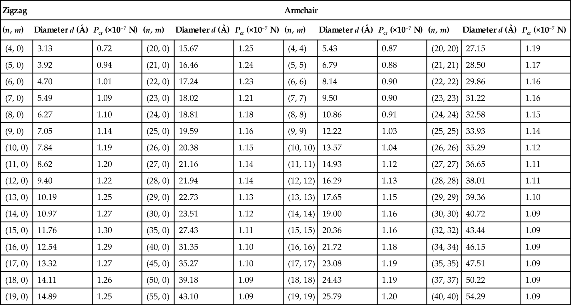
For clarity, Fig. 3.20 shows the plot of buckling load Pcr against diameter d for zigzag SWCNTs. As the diameter d of the zigzag nanotube increases, there is a rapid increase in its buckling load Pcr. However, as the diameter d reaches an optimum value d=11.76 Å, any further increment beyond that will cause the buckling load Pcr to decrease slowly to a steady value of about 1.10×10⁻⁷ N. It is evident that the length l of the CNTs will affect the critical strain ![]() .
.
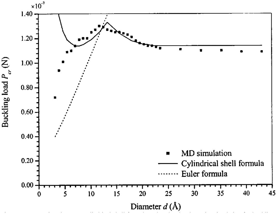
It is worthy of note that the classical shell theory can be used for the local buckling analysis of nanotubes. For a layer of cylindrical shell with length l, radius r, thickness t, Young’s modulus E, Poisson’s ratio ![]() , and m and 2n longitudinal and circumferential wave numbers, the critical stress for the buckling of the cylindrical shell is obtained as [73]
, and m and 2n longitudinal and circumferential wave numbers, the critical stress for the buckling of the cylindrical shell is obtained as [73]
(3.19)
In predicting the buckling load of nanotubes by using the cylindrical shell model, almost all previous literatures adopted the interlayer separation of graphite, i.e., t=3.4 Å as the representative thickness of single-walled nanotubes. However, the buckling loads obtained from Eq. (3.19) are much larger than our MD simulated results if t=3.4 Å is used. Here, we took the diameter of carbon atom (1.54 Å) as the thickness of the nanotube, as shown in Fig. 3.19A. The Young modulus E=1.28 TPa is directly extracted from the experimental results of Wong et al. [74] for the calculation of buckling loads using Eq. (3.19). The buckling load is not sensitive to the value of Poisson’s ratio, thus in this study, it is taken as ![]() =0.25. Using the cylindrical shell formula in Eq. (3.19) and MD, buckling loads are computed for various zigzig single-walled nanotubes, as shown in Fig. 3.20. It is observed from Fig. 3.20 that the two sets of results are in good agreement with diameter d ranging from 5.49 to 43.1 Å or larger. In spite of this, the results obtained from the cylindrical shell formula (Eq. 3.19) for diameters d smaller than 4.7 Å do not agree well with that of the MD simulation. This is because the nanotube behaves more similarly to a rod than a cylindrical shell with thickness/radius (t/r) ratio larger than 0.66. In view of this, the buckling loads of zigzag nanotubes with fixed ends are also calculated using Euler’s formula [75] and are presented in Fig. 3.20,
=0.25. Using the cylindrical shell formula in Eq. (3.19) and MD, buckling loads are computed for various zigzig single-walled nanotubes, as shown in Fig. 3.20. It is observed from Fig. 3.20 that the two sets of results are in good agreement with diameter d ranging from 5.49 to 43.1 Å or larger. In spite of this, the results obtained from the cylindrical shell formula (Eq. 3.19) for diameters d smaller than 4.7 Å do not agree well with that of the MD simulation. This is because the nanotube behaves more similarly to a rod than a cylindrical shell with thickness/radius (t/r) ratio larger than 0.66. In view of this, the buckling loads of zigzag nanotubes with fixed ends are also calculated using Euler’s formula [75] and are presented in Fig. 3.20,
(3.20)
where I is the moment of inertia. For the fixed length/diameter (l/d) ratio, the buckling loads obtained from Euler’s formula for nanotubes with fixed ends are proportional to the diameter d of nanotubes, as shown in Fig. 3.20. It is obvious from the trend that the Euler formula is more reasonable than the cylindrical shell model in the estimation of the buckling loads of nanotubes with (t/r) ratio larger than 0.66.
Fig. 3.21 plots the various critical strains ![]() of a (10, 10) SWCNT at different lengths l from 24.6 to 140.0 Å. This plot shows that as the length l increases, the critical strain
of a (10, 10) SWCNT at different lengths l from 24.6 to 140.0 Å. This plot shows that as the length l increases, the critical strain ![]() decreases. This indicates that a larger l/d ratio results in a lower critical strain
decreases. This indicates that a larger l/d ratio results in a lower critical strain ![]() .
.

 for (10, 10) single-walled carbon nanotubes with diameter of 13.57 Å at different lengths l [16].
3.4.1.2 Multiwalled carbon nanotubes
Comparisons are also made between MWCNTs to determine the effect of the number of layers on the properties of the multiwalled nanotubes. Three configurations of multiwalled nanotubes are considered in the simulation: the first is a two-walled (5, 5) and (10, 10) nanotube; the second is a three-walled (5, 5), (10, 10), and (15, 15) nanotube; and the last is a four-walled (5, 5), (10, 10), (15, 15), and (20, 20) nanotube. The lengths of all three multiwalled nanotubes are l=60 Å. And their diameters d are 13.52, 20.36, and 27.15 Å for the two-, three-, and four-walled nanotubes, respectively.
It is worth noting that the van der Waals potential is nonzero only if the covalent potential is zero, such that there is no artificial reaction barrier formed by the steep repulsive wall of the Lennard–Jones 12–6 potential to prevent nonbonded atoms from chemical reactions. The three multiwalled nanotubes are compressed axially using the same method as the single-walled nanotubes. Each time-step is equivalent to 1 fs and there are a total of 20,000 time-steps, which corresponds approximately to ![]() =0.066. The resulting plots are shown in Fig. 3.22. For multiwalled nanotubes with m layers, the total strain energy is
=0.066. The resulting plots are shown in Fig. 3.22. For multiwalled nanotubes with m layers, the total strain energy is
(3.21)
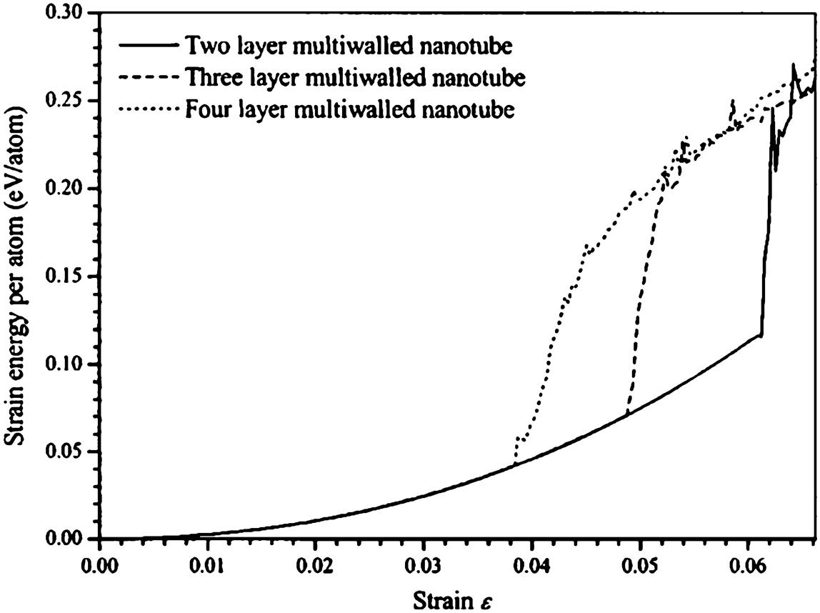
Fig. 3.22 depicts that the two-walled CNT manages to keep its elasticity for the longest with the largest critical strain at ![]() =0.06, whilst the four-walled CNT has the lowest critical strain at
=0.06, whilst the four-walled CNT has the lowest critical strain at ![]() =0.038. Instead of a spontaneous decrease of strain energy upon buckling as evidenced in the SWCNTs, the strain energy per atom increases until all the layers in the MWCNTs are fully buckled.
=0.038. Instead of a spontaneous decrease of strain energy upon buckling as evidenced in the SWCNTs, the strain energy per atom increases until all the layers in the MWCNTs are fully buckled.
The sudden increase in strain energy per atom for each layer is due to the spontaneous increase in potential energy of each atom for each layer as depicted in Fig. 3.23. From the plot, it is observed that the middle layer has the largest increment of potential energy of each atom for each layer followed by the inner layer and then the outer layer. Being sandwiched between the outer and inner layer, when the three-walled CNT starts to buckle, the atoms at the middle layer will have more nearest neighbors than those of the outer and inner layer. This causes the formation of more chemical bonds to form, from sp2 to sp3 configurations. Thus, it leads to a larger increase in the empirical bond order function and consequently the potential energy. Hence the middle layer has the highest strain energy per atom for each layer after buckling, as seen in Fig. 3.24.
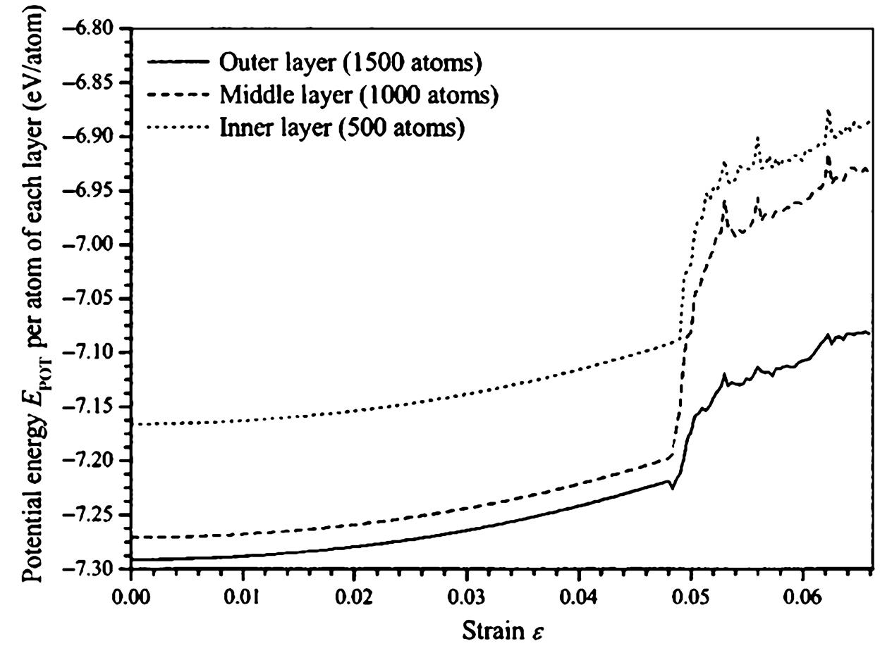
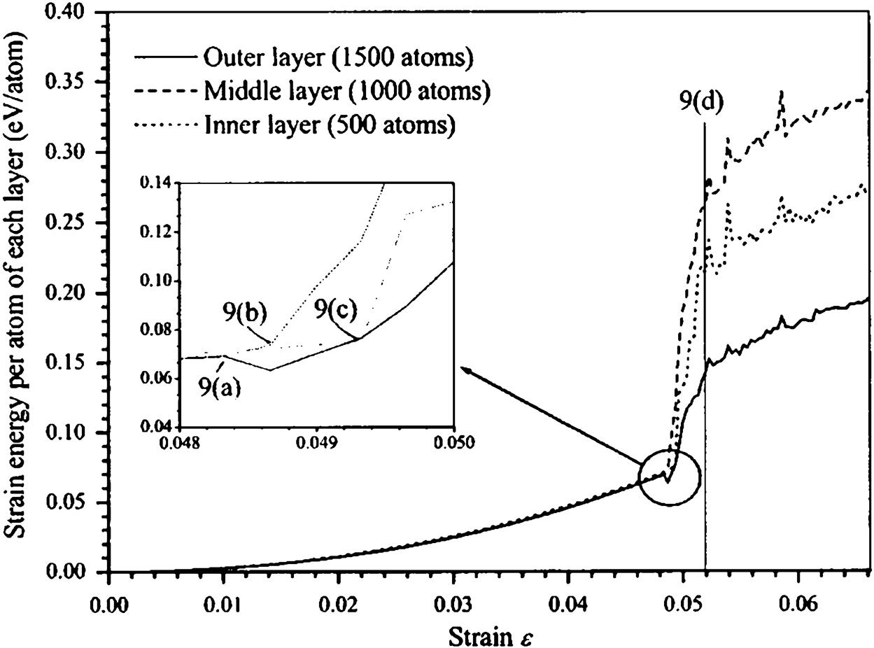
Fig. 3.25 depicts the distances of a selective pair of atoms from different layers at ![]() =0.047 (before buckling) and
=0.047 (before buckling) and ![]() =0.055 (after buckling) of the three-walled CNT. It is observed that at
=0.055 (after buckling) of the three-walled CNT. It is observed that at ![]() =0.047, the distances between the atoms from different layers are approximately 3.4 Å apart. However, at
=0.047, the distances between the atoms from different layers are approximately 3.4 Å apart. However, at ![]() =0.055, the distances between these atoms are reduced to values less than 1.6 Å. The decrease in distance allows the formation of sp3 bonds that result in a rise in the potential energy.
=0.055, the distances between these atoms are reduced to values less than 1.6 Å. The decrease in distance allows the formation of sp3 bonds that result in a rise in the potential energy.

 =0.047 and after buckling at =0.055 for the three-walled carbon nanotube [16].
To further explain the phenomenon of the increase in strain energy per atom upon buckling as observed in Fig. 3.22, the plot of the strain energy per atom for each layer of the three-walled nanotube against the strain ![]() is presented in Fig. 3.24. Before buckling, the three layers have the same strain energy per atom for each layer. However, at
is presented in Fig. 3.24. Before buckling, the three layers have the same strain energy per atom for each layer. However, at ![]() =0.0484 the outer layer starts to buckle first, followed by the middle layer at
=0.0484 the outer layer starts to buckle first, followed by the middle layer at ![]() =0.0486, and then inner layer at
=0.0486, and then inner layer at ![]() =0.0493 (see the inset of Fig. 3.24 for amplification).
=0.0493 (see the inset of Fig. 3.24 for amplification).
Fig. 3.26 shows the three-dimensional and cross-sectional three-walled nanotube at different strains. It is evident from Fig. 3.26A that the outer layer starts to deform first into a ring pattern at ![]() =0.0484, while the middle and inner layers are undeformed and their strain energies remain low. However, further compression at
=0.0484, while the middle and inner layers are undeformed and their strain energies remain low. However, further compression at ![]() =0.0486 causes the middle layer to deform too, resulting in a sudden increase in the strain energy per atom because of the increase in potential energy due to the atoms in the middle layer. Similarly at this time, the inner layer maintains the elasticity of the nanotube temporarily, as shortly after at
=0.0486 causes the middle layer to deform too, resulting in a sudden increase in the strain energy per atom because of the increase in potential energy due to the atoms in the middle layer. Similarly at this time, the inner layer maintains the elasticity of the nanotube temporarily, as shortly after at ![]() =0.0493 the inner layer also starts to buckle, therefore increasing the overall potential energy and hence further increasing the strain energy per atom further. After
=0.0493 the inner layer also starts to buckle, therefore increasing the overall potential energy and hence further increasing the strain energy per atom further. After ![]() =0.052, all the layers are deformed, hence there is no further abrupt increase in potential energy due to any sudden addition of nearest neighbors.
=0.052, all the layers are deformed, hence there is no further abrupt increase in potential energy due to any sudden addition of nearest neighbors.
 =0.0484 the outer layer deforms into a ‘‘ring’’ pattern (A). Further compression at =0.0486 causes the middle later to deform too (B). At =0.0493, the inner layer also buckles (C) and at =0.052, all the three layers are deformed (D) [16].
The force–deformation plot in Fig. 3.27 shows the buckling load Pcr that each layer is able to withstand. Being a layer with a wider diameter d, the outer layer of the three-walled CNT has the highest bucking load Pcr at about 1.18×10⁻⁷ N. However, it also tends to buckle fractionally earlier than the other two layers after deforming ![]() =2.9 Å. The buckling loads Pcr for the middle and inner layers are lower at 0.88×10⁻⁷ N and 0.42×10⁻⁷ N, respectively.
=2.9 Å. The buckling loads Pcr for the middle and inner layers are lower at 0.88×10⁻⁷ N and 0.42×10⁻⁷ N, respectively.

According to Fig. 3.28, the buckling load Pcr increases as the number of layers in a multiwalled nanotube increases. The four-walled nanotube buckles first at ![]() =2.3 Å even though it has the highest buckling load Pcr at 3.2×10⁻⁷ N; while the three-walled nanotube buckles at
=2.3 Å even though it has the highest buckling load Pcr at 3.2×10⁻⁷ N; while the three-walled nanotube buckles at ![]() =2.9 Å with Pcr=2.5×10⁻⁷ N. And finally, the two-walled nanotube buckles last at
=2.9 Å with Pcr=2.5×10⁻⁷ N. And finally, the two-walled nanotube buckles last at ![]() =3.7 Å but with the lowest buckling load Pcr=1.7×10⁻⁷ N. Hence the more layers a multiwalled nanotube has, the higher the buckling load Pcr is required.
=3.7 Å but with the lowest buckling load Pcr=1.7×10⁻⁷ N. Hence the more layers a multiwalled nanotube has, the higher the buckling load Pcr is required.
The buckling loads Pcr for two and three-walled CNTs are tabulated in Table 3.9. It is observed from the table that generally MWCNTs have larger buckling loads Pcr. For instance, the (10, 10), (15, 15) two-walled CNT has a higher buckling load Pcr=2.02×10⁻⁷ N compared to the (5, 5), (10, 10) two-walled CNT that has a buckling load Pcr=1.72×10⁻⁷ N (see Table 3.9). Moreover, Table 3.9 also verifies that as the number of layers in a CNT increases, its buckling load Pcr increases too. According to Table 3.8, the buckling load Pcr for a (5, 5) SWCNT is 0.88×10⁻⁷ N. However, if an extra outer layer is added to form a (5, 5), (10, 10) two-walled CNT, its buckling load Pcr increases to 1.72×10⁻⁷ N as seen in Table 3.9. If another layer is added to form a (5, 5), (10, 10), and (15, 15) three-walled CNT, the buckling load Pcr increases to 2.46×10⁻⁷ N.
Table 3.9
Buckling Loads for Selected Two and Three-Walled Carbon Nanotubes [16]
| Two-walled | Three-walled | ||
| (n1, m1) (n2, m2) | Pcr (×10−7N) | (n1, m1) (n2, m2) (n3, m3) | Pcr (×10−7 N) |
| (5, 5) (10, 10) | 1.72 | (5, 5) (10, 10) (15, 15) | 2.46 |
| (10, 10) (15, 15) | 2.02 | (10, 10) (15, 15) (20, 20) | 2.73 |
| (15, 15) (20, 20) | 2.09 | (15, 15) (20, 20) (25, 25) | 2.81 |
| (20, 20) (25, 25) | 2.10 | (20, 20) (25, 25) (30, 30) | 3.05 |

3.4.2 Structural Stability of a Coaxial CNTs Inside a Boron–Nitride Nanotube
Coaxial C@BNNT nanocables consisting of armchair and zigzag CNT cores and BNNT sheaths are optimized by the DFT method [76]. The structural stability is investigated by analyzing the parametric variation in the tube radius, energy, and deformation electron density. The interwall distance in the most favorable nanocables is about 0.35 nm for armchair C@BNNTs and from 0.33 to 0.36 nm for zigzag C@BNNTs. The best armchair and zigzag C@BNNTs are C(5, 5)@BN(10, 10) and C(9, 0)@BN(m, 0) (m=17, 18), respectively. The interwall interaction between CNTs and BNNTs is a typical van der Waals interaction.
3.4.2.1 Modeling method
Using C(5, 5) or C(9, 0) as the inner tube and BN(n, n) or BN(m, 0) as the outer tube, coaxial armchair C(5, 5)@BN(n, n) and zigzag C(9, 0)@BN(m, 0) nanotubes are constructed. The inner tube and outer tube are of the same tube type and possess the same repeat units. The armchair and zigzag C@BNNTs comprise eight and four basic repeat units, respectively, and the corresponding tube lengths are 1.968 and 1.704 nm. To achieve electron saturation, hydrogen atoms are used to link the two ends of the inner and outer nanotubes. Corresponding to the different diameters of the tubes, the values n=7–15 for the BN (n, n) nanotubes and m=14–22 for the BN (m, 0) nanotubes are selected.
First, the structure of the C@BNNT, its inner tube, and its outer tube are optimized. The energy and electron density are then calculated. Several representative structures of optimized C(5, 5)@BN(n, n) and C(9, 0)@BN(m, 0) structures are shown in Fig. 3.29. Energy calculation is used to quantitatively analyze the internal interaction of the structures, determine the rules governing their interaction, and elucidate the interaction mechanism. By calculating the deformation electron density, the bonding state can be intuitively understood, the bonding characterization can be analyzed, and the interaction mechanism between CNTs and BNNTs is revealed from another angle.
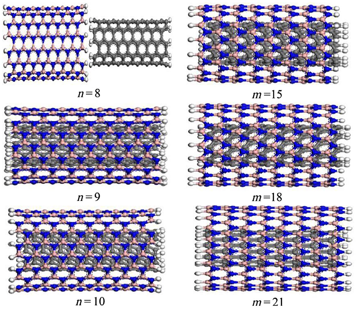
The DMol3 software is used to optimize the structure and calculate the related electrical properties [77,78]. The function PW91 [79] belonging to the generalized gradient approximation is used to process the exchange correlation potential energy, the effective core potential approach is used to process the core electron, and the orbit population parameter smearing is set at 0.0005 a.u. By using the universal force field (UFF) [80,81], several kinds of energy of the optimized structures can also be calculated. The potential energy of the UFF is expressed as the sum of bonded and nonbonded interactions.
(3.22)
The bonded interactions include the bond stretching ![]() , the angle bending
, the angle bending ![]() , the dihedral angle torsion
, the dihedral angle torsion ![]() , and the inversion terms
, and the inversion terms ![]() , respectively. The nonbonded interactions include the van der Waals interaction
, respectively. The nonbonded interactions include the van der Waals interaction ![]() and the electrostatic interaction
and the electrostatic interaction ![]() . The UFF and the parameters for C, B, and N are described in detail elsewhere in the literature [80–82].
. The UFF and the parameters for C, B, and N are described in detail elsewhere in the literature [80–82].
3.4.2.2 Structural parameters
The radii of the inner and outer nanotubes for the optimized C(5, 5)@BN(n, n) (n=9–15) are shown in Fig. 3.30 and those for C(9, 0)@BN(m, 0) (m=15–21) are shown in Fig. 3.31. Rr is the radius of the C(5, 5) or BN(n, n) in the C(5, 5)@BN(n, n) structure, and Rf is the radius of the free C(5, 5) or BN(n, n). The radial increment ![]() and the space between the inner and outer nanotubes (
and the space between the inner and outer nanotubes (![]() =Rr(BNNT)–Rr(CNT)) is the difference between the radii of the inner and outer nanotubes. The full computational details for radius of the coaxial nanotubes are given in Table 3.10.
=Rr(BNNT)–Rr(CNT)) is the difference between the radii of the inner and outer nanotubes. The full computational details for radius of the coaxial nanotubes are given in Table 3.10.