

Table 3.10
Radii (nm) of the Inner and Outer Nanotubes for the Optimized C(5, 5)@BN(n, n) and C(9, 0)@BN(m, 0) [76]
| n | BN(n, n) | C(5, 5) | |||||
| Rf | Rr | δR | Rf | Rr | δR | ||
| 9 | 0.62142 | 0.63600 | 0.01458 | 0.34094 | 0.33368 | −0.00726 | 0.30233 |
| 10 | 0.69003 | 0.68967 | −0.00036 | 0.34094 | 0.34075 | −0.00019 | 0.34892 |
| 11 | 0.75863 | 0.75624 | −0.00239 | 0.34094 | 0.34175 | 0.00081 | 0.41449 |
| 12 | 0.82712 | 0.82543 | −0.00169 | 0.34094 | 0.34143 | 0.00048 | 0.48400 |
| 13 | 0.89578 | 0.89484 | −0.00094 | 0.34094 | 0.34121 | 0.00027 | 0.55362 |
| 14 | 0.96428 | 0.96382 | −0.00047 | 0.34094 | 0.34107 | 0.00012 | 0.62275 |
| m | BN(m, 0) | C(9, 5) | |||||
| Rf | Rr | δR | Rf | Rr | δR | ||
| 15 | 0.59842 | 0.62725 | 0.02883 | 0.35409 | 0.33806 | −0.01603 | 0.28919 |
| 16 | 0.63808 | 0.6513 | 0.01322 | 0.35409 | 0.34614 | −0.00795 | 0.30515 |
| 17 | 0.67781 | 0.68094 | 0.00312 | 0.35409 | 0.35206 | −0.00203 | 0.32888 |
| 18 | 0.71744 | 0.71566 | −0.00179 | 0.35409 | 0.35451 | 0.00042 | 0.36115 |
| 19 | 0.75344 | 0.75066 | −0.00278 | 0.35409 | 0.35567 | 0.00158 | 0.39499 |
| 20 | 0.79265 | 0.79034 | −0.00231 | 0.35409 | 0.35496 | 0.00087 | 0.43537 |
| 21 | 0.83636 | 0.83453 | −0.00184 | 0.35409 | 0.3547 | 0.00060 | 0.47983 |
| 22 | 0.87612 | 0.87475 | −0.00136 | 0.35409 | 0.35452 | 0.00043 | 0.52023 |

When n=9, the radii of the outer BN(9, 9) for C(5, 5)@BN(9, 9) and of the free BN(9, 9) are 0.63600 and 0.62142 nm, respectively, the former being larger than the latter by 0.01458 nm. The radii of the inner C(5, 5) for C(5, 5)@BN(9, 9) and the free C(5, 5) are 0.33368 and 0.34094 nm, the former being less than the latter by 0.00726 nm. The space between the inner and outer nanotubes is 0.34892 nm. It is obvious that the radius of C(5, 5) decreases and that of BN(9, 9) increases when they are combined into C(5, 5)@BN(9, 9). This indicates the occurrence of greater repulsive interactions between the inner CNT and the outer BNNT. When n=10, the radii of the outer BN(10, 10) for C(5, 5)@BN(10, 10) and of the free BN(10, 10) are 0.68967 and 0.69003 nm, the former being only slightly smaller than the latter by 0.00036 nm. The radius of the inner C(5, 5) for C(5, 5)@BN(10, 10) is 0.34075 nm, which is also slightly less than that of the free C(5, 5) by 0.000194 nm. The space between the inner and outer nanotubes is 0.34892 nm. It is obvious that the radii of the inner and outer nanotubes are very close to those of the free structures. This indicates that the interaction between the inner CNT and the outer BNNT approaches zero. When n=11, the radii of the outer BN(11, 11) for C(5, 5)@BN(11, 11) and the free BN(11, 11) are 0.75624 and 0.75863 nm, the former being smaller than the latter by 0.00239 nm. The radius of the inner C(5, 5) for C(5, 5)@BN(10, 10) is 0.34175 nm, which is larger than that of the free C(5, 5) by 0.000805 nm. The space between the inner and outer nanotubes (![]() ) is 0.41449 nm. It is obvious that the radius of C(5, 5) increases and that of BN(11, 11) decreases when they are combined into C(5, 5)@BN(11, 11). This again indicates greater attraction interactions between the inner CNT and the outer BNNT. As the parameter n increases, this attraction interaction decreases gradually and tends to zero. Consequently, C(5, 5)@BN(10, 10) is a relatively stable armchair structure.
) is 0.41449 nm. It is obvious that the radius of C(5, 5) increases and that of BN(11, 11) decreases when they are combined into C(5, 5)@BN(11, 11). This again indicates greater attraction interactions between the inner CNT and the outer BNNT. As the parameter n increases, this attraction interaction decreases gradually and tends to zero. Consequently, C(5, 5)@BN(10, 10) is a relatively stable armchair structure.
The situation for the zigzag C(9, 0)@BN(m, 0) (m=15–21) nanotubes (see Fig. 3.31) is similar to that for the armchair C(5, 5)@BN(n, n) already described. As parameter m increases, the interactions between the inner CNT and the outer BNNT switch from repulsion to attraction, although the transition is smoother. The corresponding transition chiral parameter m is about 17–18 and the space between the inner and outer nanotubes (![]() ) is 0.33–0.36 nm. Thus, the most stable zigzag structures are C(9, 0)@BN(17, 0) and C(9, 0)@BN(18, 0). Nanotubes are classified as zigzag, armchair, or chiral types according to their chiral angle. The chiral angle of zigzag nanotubes is 0 degree, whereas that of armchair nanotubes is 30 degrees. The chiral angle of chiral nanotubes is within 0 and 30 degrees. Comparing the foregoing armchair C(5, 5)@BN(n, n) with zigzag C(9, 0)@BN(m, 0) (see Figs. 3.30 and 3.31), it is found that the interaction between the inner and outer tube for armchair C(5, 5)@BN(10, 10) is much closer to zero than that for zigzag C(9, 0)@BN(17, 0) or C(9, 0)@ BN(18, 0). Therefore, the optimal interwall distances in C@BNNTs are related to their chiralities. The greater the chiral angle is, the smaller the interwall interaction of combination structure is. It is obvious that the armchair C@BNNTs achieve a more stable combination structure than the zigzag case.
) is 0.33–0.36 nm. Thus, the most stable zigzag structures are C(9, 0)@BN(17, 0) and C(9, 0)@BN(18, 0). Nanotubes are classified as zigzag, armchair, or chiral types according to their chiral angle. The chiral angle of zigzag nanotubes is 0 degree, whereas that of armchair nanotubes is 30 degrees. The chiral angle of chiral nanotubes is within 0 and 30 degrees. Comparing the foregoing armchair C(5, 5)@BN(n, n) with zigzag C(9, 0)@BN(m, 0) (see Figs. 3.30 and 3.31), it is found that the interaction between the inner and outer tube for armchair C(5, 5)@BN(10, 10) is much closer to zero than that for zigzag C(9, 0)@BN(17, 0) or C(9, 0)@ BN(18, 0). Therefore, the optimal interwall distances in C@BNNTs are related to their chiralities. The greater the chiral angle is, the smaller the interwall interaction of combination structure is. It is obvious that the armchair C@BNNTs achieve a more stable combination structure than the zigzag case.
In addition, the radii of the outer BN(10, 10) in optimal C(5, 5)@BN(10, 10) and the free BN(10, 10) are 0.68967 and 0.69003 nm; the former being slightly smaller than the latter by 0.00036 nm. Thus it is concluded that the BNNT in optimal C@BNNT is hardly influenced by the combination structure. Similar to the radii of BNNT, the structural parameter of CNTs in optimal C@BN is barely affected by the coating BNNTs. They display the same fundamental characteristics as CNTs in the free space. The BNNT around the CNTs effectively helps to protect them and makes them more stable, such as oxidation degradation of CNTs is reduced by coating with BNNTs, and the thermal stability of C@BNNTs is far superior to CNTs [83–86].
To explain the interactions between the inner CNT and the outer BNNT thoroughly, the radial distribution function (RDF) of the C(5, 5) and BN(n, n) nanotubes in the C(5, 5)@BN(n, n) (n=9, 10, and 11) structure are selected for analysis (see Fig. 3.32 and Table 3.11) [22]. In the RDF of nanotubes, the peak locations (abscissa values) correspond to the first neighbor, second neighbor, and other neighbor distances between the atoms of the hexagonal atomic ring on the tube wall. Fig. 3.32 (Table 3.12) shows first and second neighbor distances for the C(5, 5) in C(5, 5)@BN(10, 10) to be 0.141 and 0.243 nm and those for the BN(10, 10) in C(5, 5)@BN(10, 10) to be 0.145 and 0.249 nm, respectively. Compared with these data in C(5, 5)@BN(10, 10), Fig. 3.32A shows that first and second neighbor distances for the C(5, 5) in C(5, 5)@BN(9, 9) are reduced to 0.139 and 0.239 nm, and the other neighbor distances also decrease. However, Fig. 3.32B shows the opposite effect for the BN(9, 9). Its first and second neighbor distances increase to 0.147 and 0.253 nm, respectively. It is clear in this case that larger mutual interactions occur between the C(5, 5) and the BN(9, 9). Fig. 3.32A and B also reveal that the first neighbor distances of the C(5, 5) increase to 0.143 nm and that of BN(11, 11) are reduced to 0.143 nm in the optimized C(5, 5)@BN(11, 11), but the second and other neighbor distances only change slightly. This indicates a weak attractive interaction between the C(5, 5) and BN(11, 11). These results concur with those shown in Fig. 3.30.
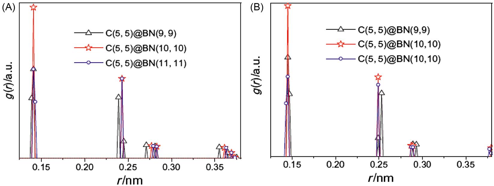
Table 3.11
Peak Locations (nm) of RDF of the C(5, 5) and BN(n, n) in C(5, 5)@BN(n, n) [76]
| Nanotubes | n | Highest Peak | Subpeak |
| C(5, 5) | 9 | 0.139 | 0.239 |
| 10 | 0.141 | 0.243 | |
| 11 | 0.143 | 0.243 | |
| BN(n, n) | 9 | 0.147 | 0.253 |
| 10 | 0.145 | 0.249 | |
| 11 | 0.143 | 0.249 |
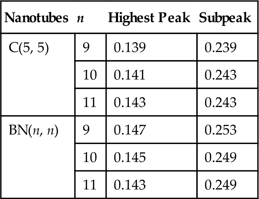
Table 3.12
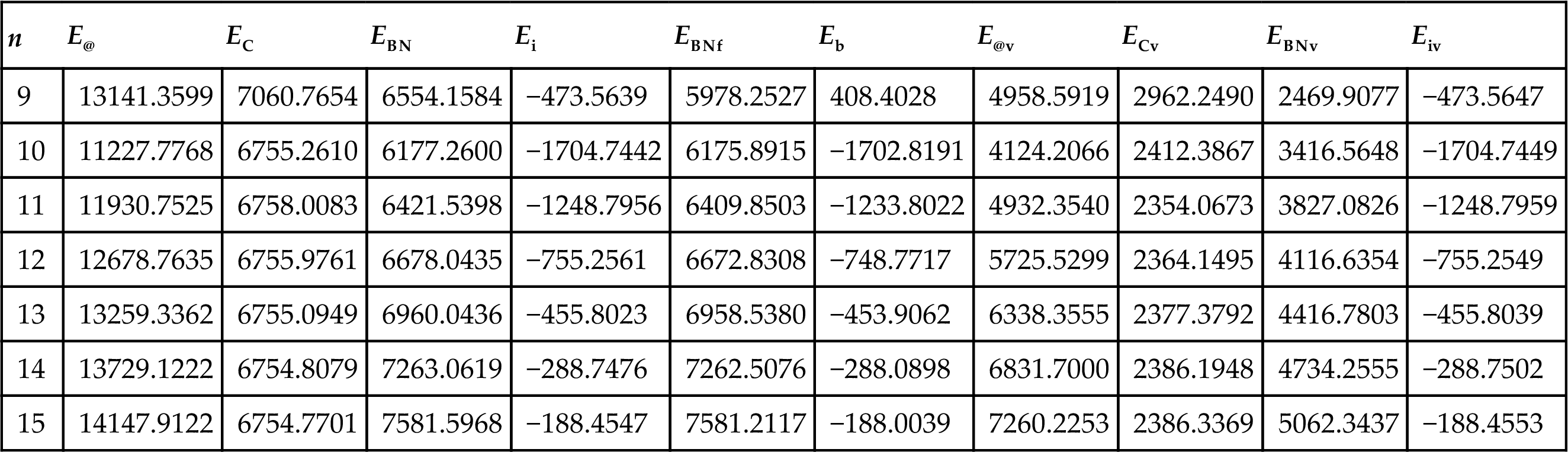
Energy of C(5, 5)@BN(n, n) and Its Inner C(5, 5) and Outer BN(n, n) (KJ/mol) [76]
| n | E@ | EC | EBN | Ei | EBNf | Eb | E@v | ECv | EBNv | Eiv |
| 9 | 13141.3599 | 7060.7654 | 6554.1584 | −473.5639 | 5978.2527 | 408.4028 | 4958.5919 | 2962.2490 | 2469.9077 | −473.5647 |
| 10 | 11227.7768 | 6755.2610 | 6177.2600 | −1704.7442 | 6175.8915 | −1702.8191 | 4124.2066 | 2412.3867 | 3416.5648 | −1704.7449 |
| 11 | 11930.7525 | 6758.0083 | 6421.5398 | −1248.7956 | 6409.8503 | −1233.8022 | 4932.3540 | 2354.0673 | 3827.0826 | −1248.7959 |
| 12 | 12678.7635 | 6755.9761 | 6678.0435 | −755.2561 | 6672.8308 | −748.7717 | 5725.5299 | 2364.1495 | 4116.6354 | −755.2549 |
| 13 | 13259.3362 | 6755.0949 | 6960.0436 | −455.8023 | 6958.5380 | −453.9062 | 6338.3555 | 2377.3792 | 4416.7803 | −455.8039 |
| 14 | 13729.1222 | 6754.8079 | 7263.0619 | −288.7476 | 7262.5076 | −288.0898 | 6831.7000 | 2386.1948 | 4734.2555 | −288.7502 |
| 15 | 14147.9122 | 6754.7701 | 7581.5968 | −188.4547 | 7581.2117 | −188.0039 | 7260.2253 | 2386.3369 | 5062.3437 | −188.4553 |
3.4.2.3 Binding energy
The stability of C@BNNT is determined by the interaction force between the inner and outer nanotubes and the deformation caused by the force. The interaction energy Ei and its van der Waals energy Eiv between the inner and outer nanotubes and the binding energy Eb of each C@BNNT are calculated, as shown in Fig. 3.33. Tables 3.12 and 3.13 show the energy of C@BNNT and its inner CNT and outer BNNT. Their total potential energies are denoted by E@, EC, and EBN, respectively, and their van der Waals energies are denoted by E@v, ECv, and EBNv, respectively. ECf and EBNf represent the total potential energy of the inner CNT and the outer BNNT in their free state. EC and EBN are obtained by calculating the single point energy of the inner CNT and the outer BNNT in a C@BNNT. The interaction energy Ei (Ei=E@–EC–EBN) between the inner and outer nanotubes is calculated. The binding energy Eb (Eb=E@–ECf–EBNf) of each C@BNNT is also calculated, in which the ECf of C(5, 5) and C(9, 0) is 6754.7044 and 5756.2738 KJ/mol, respectively. Eiv (Eiv=E@v–ECv–EBNv) denotes the van der Waals interaction between the inner and outer nanotubes, and is a component of the interaction energy Ei.
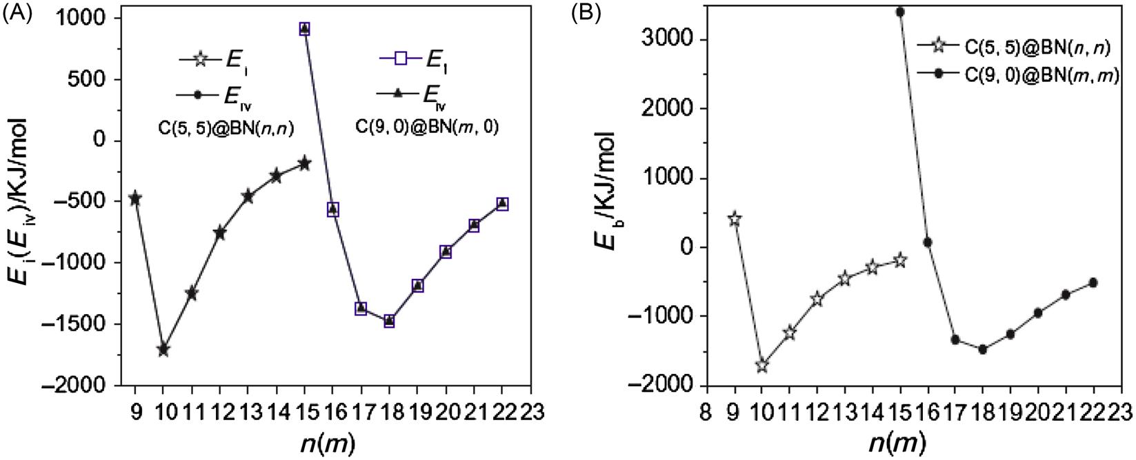
Table 3.13
Energy of C(9, 0)@BN(m, 0) and Its Inner C(9, 0) and Outer BN(m, 0) (KJ/mol) [76]
| m | E@ | EC | EBN | Ei | EBNf | Eb | E@v | ECv | EBNv | Eiv |
| 15 | 14466.7376 | 6775.0002 | 6783.2829 | 908.4545 | 5312.3118 | 3398.152 | 5602.8929 | 3053.4566 | 1640.9844 | 908.4519 |
| 16 | 10782.8325 | 5990.191 | 5355.8065 | −563.165 | 4954.4244 | 72.1343 | 4110.6857 | 2504.7563 | 2169.094 | −563.1646 |
| 17 | 9450.1524 | 5773.1001 | 5048.7748 | −1371.7225 | 5026.822 | −1332.9434 | 3484.2938 | 2203.1192 | 2652.8955 | −1371.7209 |
| 18 | 9395.5699 | 5757.1002 | 5115.2682 | −1476.7985 | 5110.5014 | −1471.2053 | 3582.4326 | 2083.3956 | 2975.834 | −1476.797 |
| 19 | 9761.4202 | 5759.2165 | 5191.5173 | −1189.3136 | 5258.5779 | −1253.4315 | 4205.3893 | 2065.6473 | 3329.6584 | −1189.9164 |
| 20 | 10198.1675 | 5758.4794 | 5348.434 | −908.7459 | 5389.3492 | −947.4555 | 4656.3946 | 2065.8981 | 3499.2452 | −908.7487 |
| 21 | 10485.9898 | 5757.5615 | 5419.4814 | −691.0531 | 5414.5755 | −684.8595 | 4820.8316 | 2070.1659 | 3441.7242 | −691.0585 |
| 22 | 10773.8162 | 5756.9206 | 5532.3457 | −515.4501 | 5529.9226 | −512.3802 | 5139.7949 | 2075.9928 | 3579.2546 | −515.4525 |
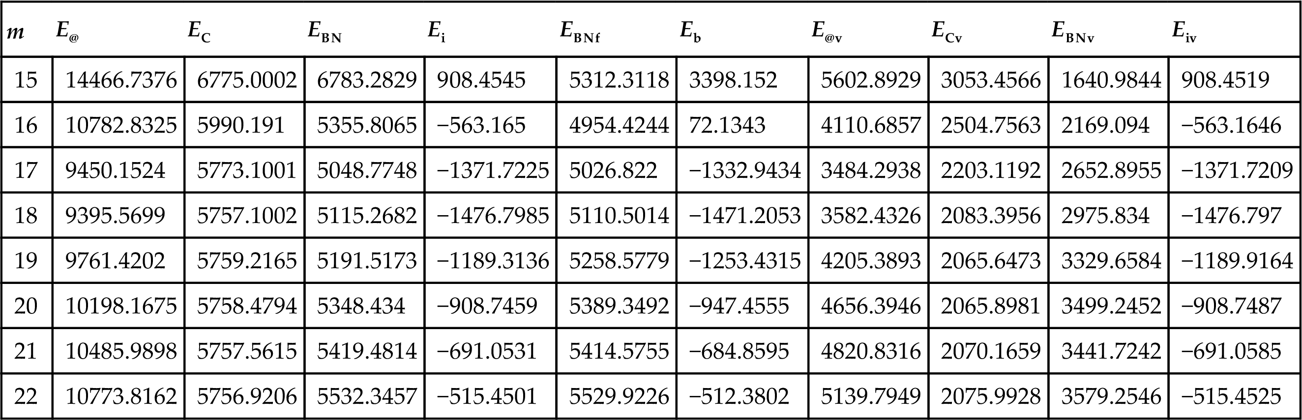
Fig. 3.33 shows that Eb is a positive value only when n=9, m=16. This indicates that the interaction force between the inner CNT and outer BNNT is one of repulsion. However, the interaction energy remains slightly negative. Only when m(n) is further reduced does a positive Eb occur. This is probably because the single point energy of the inner CNT and the outer BNNT in a C@BNNT is influenced by the H bond at either ends of the actual deformation, which means that the computed values of EC and EBN are slightly larger than their actual values. For a C@BNNT with ![]() ,
, ![]() , Eb and Ei are always negative. This indicates that the interaction between the inner and outer nanotubes is one of attraction. Fig. 3.33 shows the curves for Ei and Eb with different n(m) for C(5, 5)@BN(n, n) and C(9, 0)@BN(m, 0). It can be clearly seen from the figure that the greatest attraction is displayed at n=10 for C(5, 5)@B(n, n) and at m=17–18 for C(9, 0)@BN(m, 0). At this point, the space between the tube walls for the armchair and zigzag C@BNNTs are about 0.35 and 0.33–0.36 nm, respectively. These values are just within the distance between the layers of 0.33–0.36 nm for graphite and h-BN. When
, Eb and Ei are always negative. This indicates that the interaction between the inner and outer nanotubes is one of attraction. Fig. 3.33 shows the curves for Ei and Eb with different n(m) for C(5, 5)@BN(n, n) and C(9, 0)@BN(m, 0). It can be clearly seen from the figure that the greatest attraction is displayed at n=10 for C(5, 5)@B(n, n) and at m=17–18 for C(9, 0)@BN(m, 0). At this point, the space between the tube walls for the armchair and zigzag C@BNNTs are about 0.35 and 0.33–0.36 nm, respectively. These values are just within the distance between the layers of 0.33–0.36 nm for graphite and h-BN. When ![]() and
and ![]() , the attraction between the inner CNT and the outer BNNT begins to decline. As Eb is the energy change when the free CNT and free BNNT are bound together as a C@BNNT system, n=9 and m=15 and 16 result in endothermic processes, and the rest are exothermic processes. The heat of the exothermic process is highest when n=10 and m=17–18. This indicates that the systems with n=10 and m=17–18 are most stable. The difference between Ei and Eb reflects the energy loss caused by the deformation of the CNT and BNNT when the free CNT and free BNNT are bound together as a C@BNNT. Fig. 3.33 shows that the maximal energy loss takes place in the C@BNNT, where n=9 and m=15 and 16. This is because there is greater repulsion between the inner and outer nanotubes, which leads to greater deformation and results in a larger energy loss. It should be noted that when n=8 (not shown in the Fig. 3.33), the C(5, 5)@BN(n, n) structure cannot be maintained because of the powerful repulsion between the inner and outer tubes. The optimal structure occurs with a separation along the axial direction (see Fig. 3.29). When
, the attraction between the inner CNT and the outer BNNT begins to decline. As Eb is the energy change when the free CNT and free BNNT are bound together as a C@BNNT system, n=9 and m=15 and 16 result in endothermic processes, and the rest are exothermic processes. The heat of the exothermic process is highest when n=10 and m=17–18. This indicates that the systems with n=10 and m=17–18 are most stable. The difference between Ei and Eb reflects the energy loss caused by the deformation of the CNT and BNNT when the free CNT and free BNNT are bound together as a C@BNNT. Fig. 3.33 shows that the maximal energy loss takes place in the C@BNNT, where n=9 and m=15 and 16. This is because there is greater repulsion between the inner and outer nanotubes, which leads to greater deformation and results in a larger energy loss. It should be noted that when n=8 (not shown in the Fig. 3.33), the C(5, 5)@BN(n, n) structure cannot be maintained because of the powerful repulsion between the inner and outer tubes. The optimal structure occurs with a separation along the axial direction (see Fig. 3.29). When ![]() or
or ![]() , the distances between the inner and outer nanotubes increase, and the deformation and energy loss decrease rapidly. In the formation of the C(5, 5)@BN(n, n) and C(9, 0)@BN(m, 0) systems, the energy change derives mainly from the interaction force between molecules, and the effect of deformation on the energy change is slight. A comparison of Ei and Eiv in Fig. 3.33 shows that the difference is very small. It can thus be concluded that the interaction between the inner CNT and outer BNNT is a typical van der Waals interaction between molecules.
, the distances between the inner and outer nanotubes increase, and the deformation and energy loss decrease rapidly. In the formation of the C(5, 5)@BN(n, n) and C(9, 0)@BN(m, 0) systems, the energy change derives mainly from the interaction force between molecules, and the effect of deformation on the energy change is slight. A comparison of Ei and Eiv in Fig. 3.33 shows that the difference is very small. It can thus be concluded that the interaction between the inner CNT and outer BNNT is a typical van der Waals interaction between molecules.
3.4.2.4 Electronic structure and bonding model
To further understand the interaction between the CNT and BNNT in a C@BNNT, the deformation electron density and its isoline structure are calculated. As the effects of different values of the parameter n(m) on the electronic distribution of C(5, 5)@BN(n, n) and C(9, 0)@BN(m, 0) follow a similar law, only C(5, 5)@BN(n, n) is used in the analysis. Fig. 3.34 shows the deformation electron density and its section isoline as calculated by DFT by simulating a C(5, 5)@BN(n, n) model for n=9, 10, and 11. The electron density is the same as the online equivalent, and gradually becomes smaller on the vertical isolines from the inside outward. The isoline intervals reflect the local electronic conditions, in that the greater the interval, the weaker the localization and the more free the electrons, and vice versa.
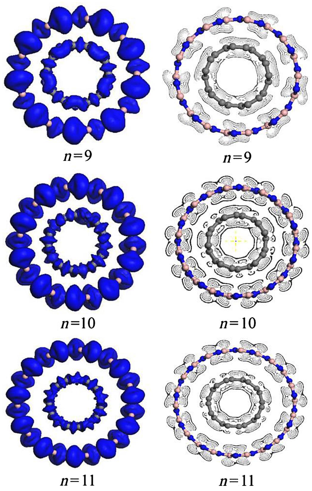
As shown in Fig. 3.34, in the outer tube BN(n, n)NT, the outer-layer electrons are obviously partial to the N atom in the B–N bond. However, in the inner CNT, the electrons are more concentrated at the center of the C–C bond. The outer-layer electrons are the main cause of the covalent bond. If the outer-layer electrons spend most of their time within the nuclei of the two atoms, then the covalent bond is placed in the bonding orbital, in which case the distribution shape of the electron density is small at either end and large in the middle. In contrast, if the electrons spend most of their time outside the nuclei of the two atoms, then the covalent bond is placed in the antibonding orbital, in which case the distribution shape of the electron density is large at either end and small in the middle. This is because in the bonding orbital there is an increase in electron density between the nuclei, whereas in the antibonding orbital there is a decrease in electron density. Placing an electron in the bonding orbital stabilizes the molecule because it remains in between the two nuclei. Conversely, placing electrons in the antibonding orbital cause a decrease in stability [87]. The deformation electron density plot in Fig. 3.34 shows that C(5, 5)@BN(10, 10)NT has a good bonding electronic distribution that is small at either end and large in the middle. The electrons are uniformly distributed along the atoms in rings. The shape when n=11 is similar to that when n=10, but is different when n=9. This is mainly because a part of the bond of the inner CNT shows an antibonding effect. The isoline structure in Fig. 3.34 shows some regular change as the parameter n increases. For example, when n=9, because of the repulsive interactions between the inner CNT and the outer BNNT, some of the outer electrons tend toward the inside. Consequently, the isoline interval is smaller and a partial antibonding effect may occur. When n=10, the repulsive interactions disappear, the outer layer regains its electron density, the isoline interval is medium-sized, and it is difficult for the antibonding effect to occur. The electron distribution also has a good bonding characterization. Thus, the structural stability of C(5, 5)@BN(10, 10) is superior to that of C(5, 5)@BN(9, 9). When n=11, due to the attraction between the CNT and the BNNT, the electronic localization of the inner layer may be weakened, some s electrons become p electrons due to excitation, and partial electronic delocalization of the outer layer occurs, which results in an increase in electron mobility. Consequently, the outside electron density for n=11 decreases and the isoline interval for the inner layer become somewhat sparse. Of course, as this effect is small, the electron density distribution is still similar to that when n=10. In general, the numbers of nonlocalized outer-layer electrons, which are related to the conductivity, increase, and the number of bonding electrons, which maintain the stability of the structure, naturally decrease. Thus, the structural stability of C(5, 5)@BN(10, 10) is superior to that of C(5, 5)@BN(11, 11).
Fig. 3.34 clearly shows that bonding electronic distributions are only formed between B and N or C and C, and no bond is formed between B and C or N and C. The distribution state remains basically unchanged despite changes in parameter n. This indicates that there is no bond mix between the CNT and the BNNT in a C@BNNT, and the interactions between the CNT and BNNT are only van der Waals forces between the molecules. This result concurs with the conclusion drawn from the energy analysis.
3.5 Buckling of CNTs Bundles
In the MD simulations of CNT bundles, the analysis was carried out without considering temperature control. Axial tension and compression of the perfectly structured CNT bundles were achieved by applying a constant rate of 20 m/s at both ends. At the beginning of each simulation, the CNT bundle was allowed to equilibrate before proceeding into the “production phase” where the trajectories of the atoms, energies, and forces were extracted and later analyzed. The end atoms were then shifted either inwardly (compression) or outwardly (tension) along the axis by small steps and the whole CNT bundle was subsequently relaxed by a conjugate gradient minimization method, while keeping the end atoms fixed. This process repeats until the CNT bundle breaks. Each simulation had a total of 25,000 time-steps, and each simulation time-step is equivalent to 1 fs.
The algorithm was implemented in parallel by a domain decomposition method, i.e., dividing a CNT bundle lengthwise across individual processors of the computer. A Message-Passing Interface library [88] was used in the parallelization for communication of data. The MD simulations reported here were run on parallel platforms using four processors on SGI Origin 3400, to reduce computation time significantly.
To obtain an insight into the buckling behavior of the CNT bundles, two sets of MD simulations were carried out for each size of CNT bundle, i.e., with and without the long-range nonbonding van der Waals interactions. Fig. 3.35 shows the plot of the buckling load Pcr against the CNT bundle size. From the plot, we can see a linear relationship between the buckling load Pcr and the CNT bundle size, with a bigger CNT bundle size having a larger buckling load Pcr. For instance, a CNT bundle with four SWCNTs has a buckling load of Pcr=0.527×10⁻⁶ N, while a CNT bundle with 25 SWCNTs has a much larger buckling load at Pcr=3.30×10⁻⁶ N. For comparison, a (10, 10) SWCNT is included in the plot, which reveals that the addition of more SWCNTs to a CNT bundle enhances its rigidity because the total cross-sectional area increases, and hence greater force is needed to buckle the bundle, leading to an increase in its buckling load Pcr.

Fig. 3.35 also shows the buckling loads Pcr of the CNT bundles without considering the long-range nonbonding van der Waals interactions. When the long-range interactions are not considered, the buckling loads Pcr of the bundles drop by a small percentage. The buckling loads Pcr of the various CNT bundles with and without consideration of the long-range nonbonding van der Waals interactions are listed in Table 3.14.
Table 3.14
Buckling Loads Pcr of Different Sizes of CNT Bundles With and Without van der Waals Interactions and Their Difference (in Percentage) [14]
| CNT Bundle Size | Buckling Load Pcr | Differences in Percentage (%) | |
| Without van der Waals (×10−6 N) | With van der Waals (×10−6 N) | ||
| 1 | 0.130 | 0.136 | 4.6 |
| 4 | 0.520 | 0.540 | 3.8 |
| 9 | 1.170 | 1.220 | 4.3 |
| 16 | 2.070 | 2.170 | 4.8 |
| 25 | 3.240 | 3.410 | 5.2 |
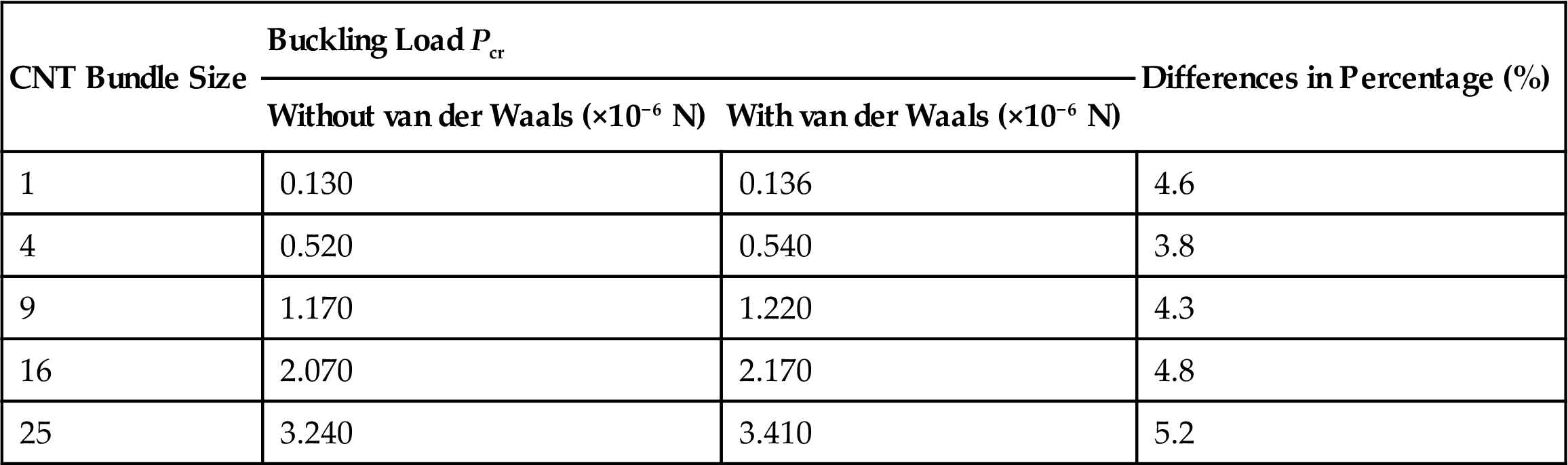
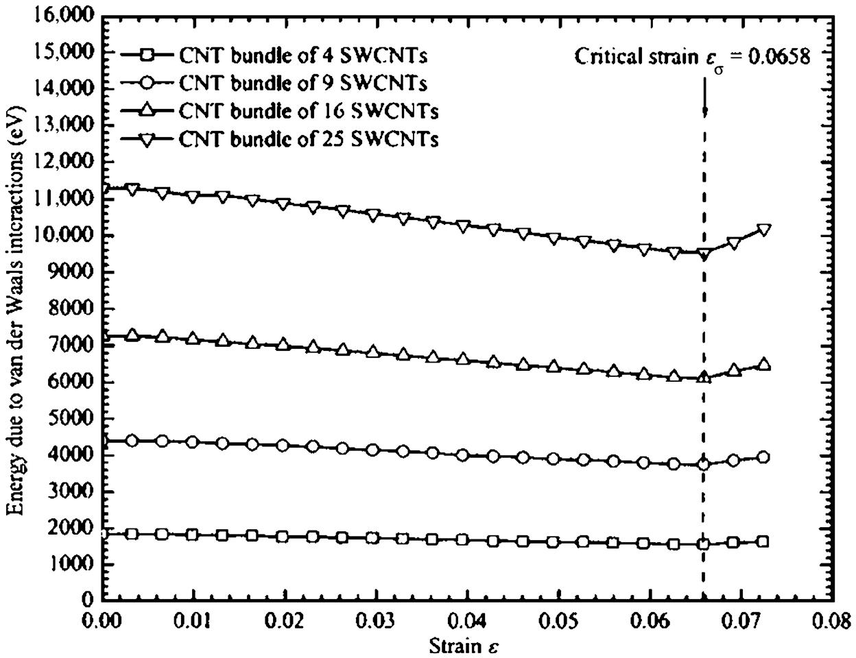
The inclusion of long-range nonbonding van der Waals interactions has a strengthening effect and thereby increases the buckling loads Pcr of the various CNT bundles by about 3.8–5.2%. The importance of van der Waals interactions increases as the size of the CNT bundle increases. Fig. 3.36 shows the total energy due to van der Waal interactions for different sizes of CNT bundles. The biggest CNT bundle of 25 SWCNTs has the largest van der Waals potential because of the larger interspacial gaps, while the CNT bundle of four SWCNTs has the lowest van der Waals potential. Hence, greater van der Waals interactions due to larger interspacial gaps contribute to a strengthening effect, which results in an improvement in the buckling load Pcr of CNT bundles.
 for different sizes of CNT bundles [14].
It is also evident in Table 3.14 that even without taking into account van der Waals interactions, the inclusion of more SWCNTs in a CNT bundle already has a large influence on its buckling load Pcr. For example, the buckling load Pcr of a CNT bundle with 25 SWCNTs is five times larger that of a CNT with four SWCNTs without considering van der Waals interactions. Hence, even though the van der Waal interactions play an important role in strengthening the CNT bundle, the addition of extra SWCNTs more significantly contributes to the overall strength of the bundle.
From Fig. 3.35, we can also see that the buckling load Pcr of a CNT bundle is proportional to that of an SWCNT. For instance, the buckling load Pcr of a (10, 10) SWCNT is about 0.136×10⁻⁶ N (see Table 3.14) and a CNT bundle of four (10, 10) SWCNTs has a buckling load Pcr four times higher than that of an SWCNT. Hence, it would be useful to determine for any size of CNT bundle whether the buckling load ![]() is the product of the buckling load
is the product of the buckling load ![]() of a similar SWCNT and the total number of SWCNTs in the CNT bundle. Therefore,
of a similar SWCNT and the total number of SWCNTs in the CNT bundle. Therefore,
(3.23)
where n is the total number of SWCNTs in a CNT bundle, ![]() is the buckling load of a CNT bundle and
is the buckling load of a CNT bundle and ![]() is the buckling load of an SWCNT.
is the buckling load of an SWCNT.
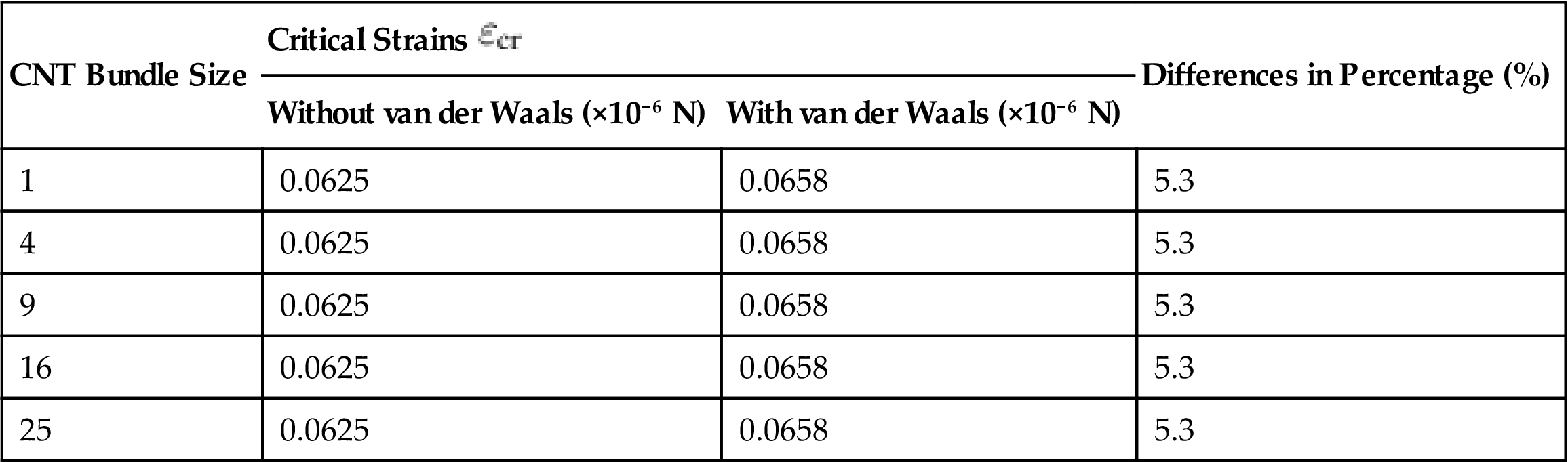
The critical strains ![]() at which the CNT bundles buckle were also investigated (see Table 3.15). Being a strengthening mechanism, the van der Waals interactions delay the collapse of the CNT bundle by creating weak intertube bonds due to the intertube attractive forces. Despite the different sizes of CNT bundles, they all had the same critical strains of
at which the CNT bundles buckle were also investigated (see Table 3.15). Being a strengthening mechanism, the van der Waals interactions delay the collapse of the CNT bundle by creating weak intertube bonds due to the intertube attractive forces. Despite the different sizes of CNT bundles, they all had the same critical strains of ![]() =0.0658 and
=0.0658 and ![]() =0.0625 for those with and without long-range van der Waals interactions.
=0.0625 for those with and without long-range van der Waals interactions.
Table 3.15
Critical Strains ![]() of Different Sizes of CNT Bundles With and Without van der Waals Interactions and Their Difference (In Percentage) [14]
of Different Sizes of CNT Bundles With and Without van der Waals Interactions and Their Difference (In Percentage) [14]
| CNT Bundle Size | Critical Strains |
Differences in Percentage (%) | |
| Without van der Waals (×10−6 N) | With van der Waals (×10−6 N) | ||
| 1 | 0.0625 | 0.0658 | 5.3 |
| 4 | 0.0625 | 0.0658 | 5.3 |
| 9 | 0.0625 | 0.0658 | 5.3 |
| 16 | 0.0625 | 0.0658 | 5.3 |
| 25 | 0.0625 | 0.0658 | 5.3 |
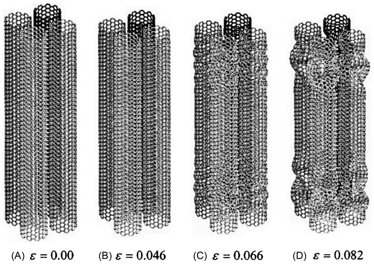
The morphological deformation of the CNT bundles when compressed was also investigated. During compression, CNT bundles undergo structural deformation. Fig. 3.37 shows the morphological changes at various stages of the compression process for the CNT bundle consisting of four SWCNTs. At strain ![]() =0.00, the CNT bundle remains at its original length as shown in Fig. 3.37A. Further compression until
=0.00, the CNT bundle remains at its original length as shown in Fig. 3.37A. Further compression until ![]() =0.046 reveals an overall decrease in length lt of the CNT bundle (Fig. 3.37B). At
=0.046 reveals an overall decrease in length lt of the CNT bundle (Fig. 3.37B). At ![]() =0.066, each SWCNT in the CNT bundle begins to buckle and spontaneously collapse into “ring” patterns as revealed in Fig. 3.37C. At
=0.066, each SWCNT in the CNT bundle begins to buckle and spontaneously collapse into “ring” patterns as revealed in Fig. 3.37C. At ![]() =0.082, the whole CNT bundle is fully buckled (Fig. 3.37D).
=0.082, the whole CNT bundle is fully buckled (Fig. 3.37D).
 [14].
[14].In summary, the mechanical properties, in particular the critical buckling load Pcr and critical strain ![]() , of different sizes of CNT bundles, were studied using MD simulations. We found that the buckling loads Pcr of CNT bundles are much higher than that of an SWCNT. At the same time, the bigger the CNT bundle, the higher the buckling load Pcr. Additionally, the critical strains
, of different sizes of CNT bundles, were studied using MD simulations. We found that the buckling loads Pcr of CNT bundles are much higher than that of an SWCNT. At the same time, the bigger the CNT bundle, the higher the buckling load Pcr. Additionally, the critical strains ![]() of the CNT bundles are not affected by their sizes. It was also deduced that the van der Waals interactions play a role in strengthening the overall rigidity of the CNT bundle. Depending on the size of the CNT bundle, the van der Waals interactions improve the buckling load Pcr by more than 3.8%, and the critical strain
of the CNT bundles are not affected by their sizes. It was also deduced that the van der Waals interactions play a role in strengthening the overall rigidity of the CNT bundle. Depending on the size of the CNT bundle, the van der Waals interactions improve the buckling load Pcr by more than 3.8%, and the critical strain ![]() by about 5.3%. The buckling load Pcr of a CNT bundle was also found to be directly proportionally to that of an SWCNT.
by about 5.3%. The buckling load Pcr of a CNT bundle was also found to be directly proportionally to that of an SWCNT.
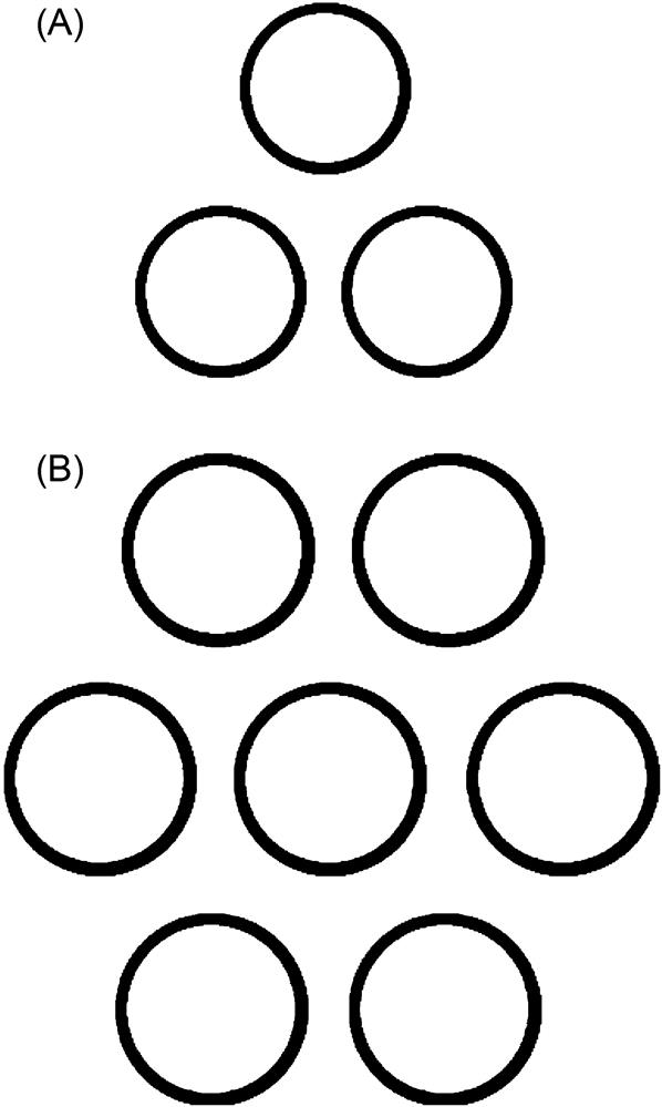
Fig. 3.38 shows the schematic of two CNT bundles used in the MD simulations. The CNT bundle consisted of three or seven individual SWCNTs vertically aligned next to one another. In the MD simulations, various sizes of CNT bundles were used. These sizes were determined by the size of the individual SWCNTs in the bundle.
3.5.1 CNT Bundles Under Axial Tension
In the MD simulations of CNT bundles under axial tension, altogether there were four sizes of SWCNTs used, namely (5, 5), (7, 7), (10, 10), and (12, 12) SWCNTs. The interspacial gap between the individual SWCNTs in the CNT bundle was fixed at 0.34 nm.
During tensile loading, the CNT bundles undergo structural deformation as shown in Fig. 3.39. Fig. 3.39A shows that there was no structural deformation in both CNT bundles of three and seven (10, 10) SWCNTs at strain ![]() =0.0. When the CNT bundles are further subjected to tensile force as seen in Fig. 3.39B, and at strain
=0.0. When the CNT bundles are further subjected to tensile force as seen in Fig. 3.39B, and at strain ![]() =0.130, the CNT bundles tend to shrink their overall diameter along their lengths. At strain
=0.130, the CNT bundles tend to shrink their overall diameter along their lengths. At strain ![]() =0.266, both CNT bundles begin to fracture before they completely disintegrate.
=0.266, both CNT bundles begin to fracture before they completely disintegrate.

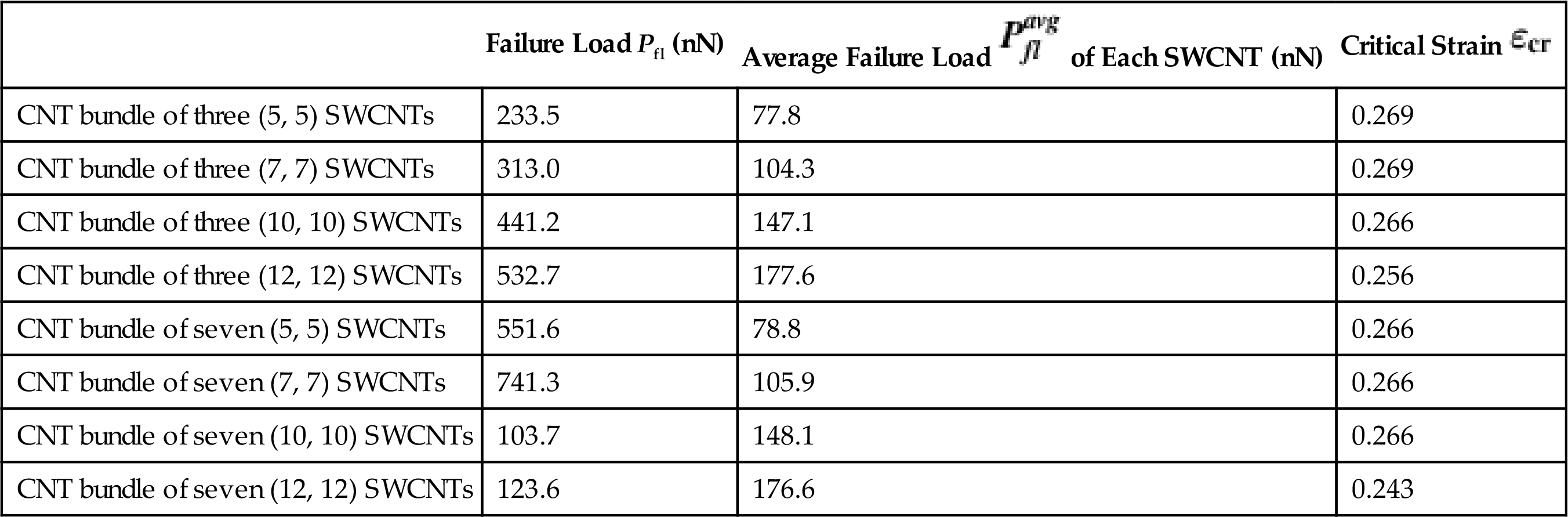
Fig. 3.40 depicts the failure loads Pfl of various sizes of the CNT bundles of three and seven SWCNTs, respectively. The plots clearly demonstrate that CNT bundles with larger SWCNTs exhibit higher failure loads Pfl. From the plots and Table 3.16, it is also evident that the average failure load ![]() of each SWCNT in a CNT bundle of three is very close to that of a CNT bundle of seven. It can therefore be deduced that the critical failure loads Pfl for CNT bundles are directly proportional to the average critical failure load
of each SWCNT in a CNT bundle of three is very close to that of a CNT bundle of seven. It can therefore be deduced that the critical failure loads Pfl for CNT bundles are directly proportional to the average critical failure load ![]() of each SWCNT in the CNT bundle. This information allows simple computation of CNT bundles of up to hundreds of SWCNTs without having to perform computationally expensive MD simulations with millions of atoms. For instance, the average critical failure loads
of each SWCNT in the CNT bundle. This information allows simple computation of CNT bundles of up to hundreds of SWCNTs without having to perform computationally expensive MD simulations with millions of atoms. For instance, the average critical failure loads ![]() of a CNT bundle of three and seven (10, 10) SWCNTs are 147.1 and 148.1 nN, respectively (according to Table 3.16). Hence, the critical failure load Pfl of a CNT bundle of twenty (10, 10) SWCNTs is approximated to be 294.2 nN.
of a CNT bundle of three and seven (10, 10) SWCNTs are 147.1 and 148.1 nN, respectively (according to Table 3.16). Hence, the critical failure load Pfl of a CNT bundle of twenty (10, 10) SWCNTs is approximated to be 294.2 nN.
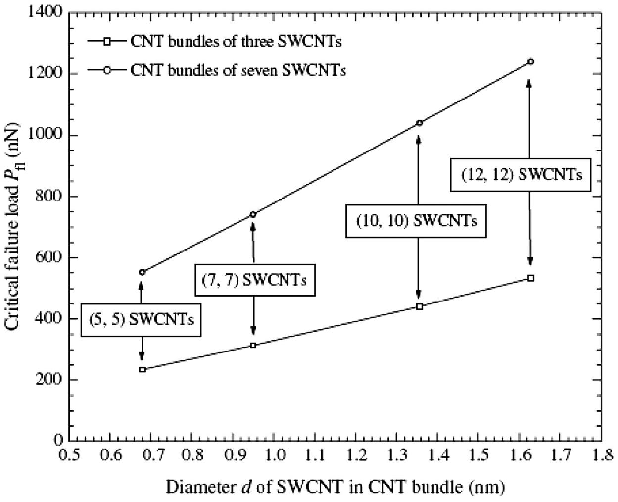
Table 3.16
Failure Loads Pfl and Critical Strains ![]() of Various Configurations of CNT Bundles [15]
of Various Configurations of CNT Bundles [15]
| Failure Load Pfl (nN) | Average Failure Load |
Critical Strain | |
| CNT bundle of three (5, 5) SWCNTs | 233.5 | 77.8 | 0.269 |
| CNT bundle of three (7, 7) SWCNTs | 313.0 | 104.3 | 0.269 |
| CNT bundle of three (10, 10) SWCNTs | 441.2 | 147.1 | 0.266 |
| CNT bundle of three (12, 12) SWCNTs | 532.7 | 177.6 | 0.256 |
| CNT bundle of seven (5, 5) SWCNTs | 551.6 | 78.8 | 0.266 |
| CNT bundle of seven (7, 7) SWCNTs | 741.3 | 105.9 | 0.266 |
| CNT bundle of seven (10, 10) SWCNTs | 103.7 | 148.1 | 0.266 |
| CNT bundle of seven (12, 12) SWCNTs | 123.6 | 176.6 | 0.243 |
The figure also shows that the critical failure loads Pfl follow an almost linear relationship with respect to the diameters d of each SWCNT in the CNT bundles. This enables the determination of critical failure loads Pfl of other sizes of CNT bundles by simply extrapolating the data.
The critical strains ![]() at which these CNT bundles fail are also presented in Table 3.16. From the table, it can be observed that the critical strains
at which these CNT bundles fail are also presented in Table 3.16. From the table, it can be observed that the critical strains ![]() are relatively insensitive to the various CNT bundles, despite the difference in their size and total number of SWCNTs in the CNT bundles. Although the critical strains
are relatively insensitive to the various CNT bundles, despite the difference in their size and total number of SWCNTs in the CNT bundles. Although the critical strains ![]() are generally within 0.266–0.269, further studies are needed to understand why they drop to 0.243 and 0.256 for CNT bundles of three and seven (12, 12) SWCNTs, respectively.
are generally within 0.266–0.269, further studies are needed to understand why they drop to 0.243 and 0.256 for CNT bundles of three and seven (12, 12) SWCNTs, respectively.
3.5.2 CNT Bundles Under Axial Compression
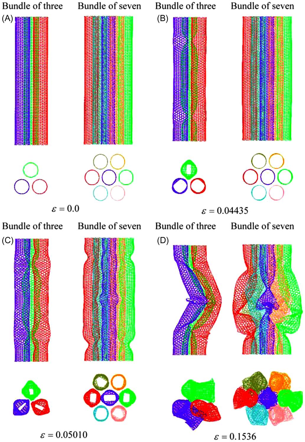
When compressed, the CNT bundles will undergo structural deformation. Fig. 3.41 shows the morphological changes at various stages of the compression process of CNT bundles of three and seven (10, 10) SWCNTs. Fig. 3.41A shows the CNT bundles at strain ![]() =0.0, where there is no deformation. Further compression until strain
=0.0, where there is no deformation. Further compression until strain ![]() =0.04435 will cause the CNT bundle of three to spontaneously collapse into a three-fin pattern, while the CNT bundle of seven is bent slightly outwards from the core SWCNT. At strain
=0.04435 will cause the CNT bundle of three to spontaneously collapse into a three-fin pattern, while the CNT bundle of seven is bent slightly outwards from the core SWCNT. At strain ![]() =0.05010, the CNT bundle of three continues to deform. However, the CNT bundle of seven begins to buckle forming three-fin patterns in each of its SWCNTs. Finally at strain
=0.05010, the CNT bundle of three continues to deform. However, the CNT bundle of seven begins to buckle forming three-fin patterns in each of its SWCNTs. Finally at strain ![]() =0.1536, the CNT bundle of three buckles sideways at the same direction, while the CNT bundle of seven buckles outwards from its core SWCNT forming a “birdcage” pattern.
=0.1536, the CNT bundle of three buckles sideways at the same direction, while the CNT bundle of seven buckles outwards from its core SWCNT forming a “birdcage” pattern.
Investigations were carried out on the buckling properties of CNT bundles. Altogether, seven sizes of CNT bundles were used. They are namely (5, 5), (7, 7), (10, 10), (12, 12), (15, 15), (18, 18), and (20, 20). The plot in Fig. 3.42 shows the critical buckling loads Pcr for the different sizes of CNT bundles of three and seven. From the plot, it can be seen that as the size of the individual SWCNT in a CNT bundle increases, its buckling load Pcr also increases exponentially. Also, the critical buckling load Pcr of the CNT bundles of three tends to reach a maximum value of ![]() 300 nN despite further increases in the diameters d.
300 nN despite further increases in the diameters d.

However, the CNT bundles with seven SWCNTs have critical buckling loads Pcr of about two to three times higher than that of CNT bundles of three SWCNTs. As the diameters d of the SWCNTs in the CNT bundle of seven increase, the difference in critical buckling loads Pcr between the CNT bundles of three and seven SWCNTs also increases. For instance, at diameter d=0.68 nm, the critical buckling load Pcr of the CNT bundle of seven (5, 5) SWCNTs is about 2.1 times larger. However, when the diameter increases to d=2.44 nm, the critical buckling load Pcr of the CNT bundle of seven (18, 18) SWCNTs is about 2.4 times larger.
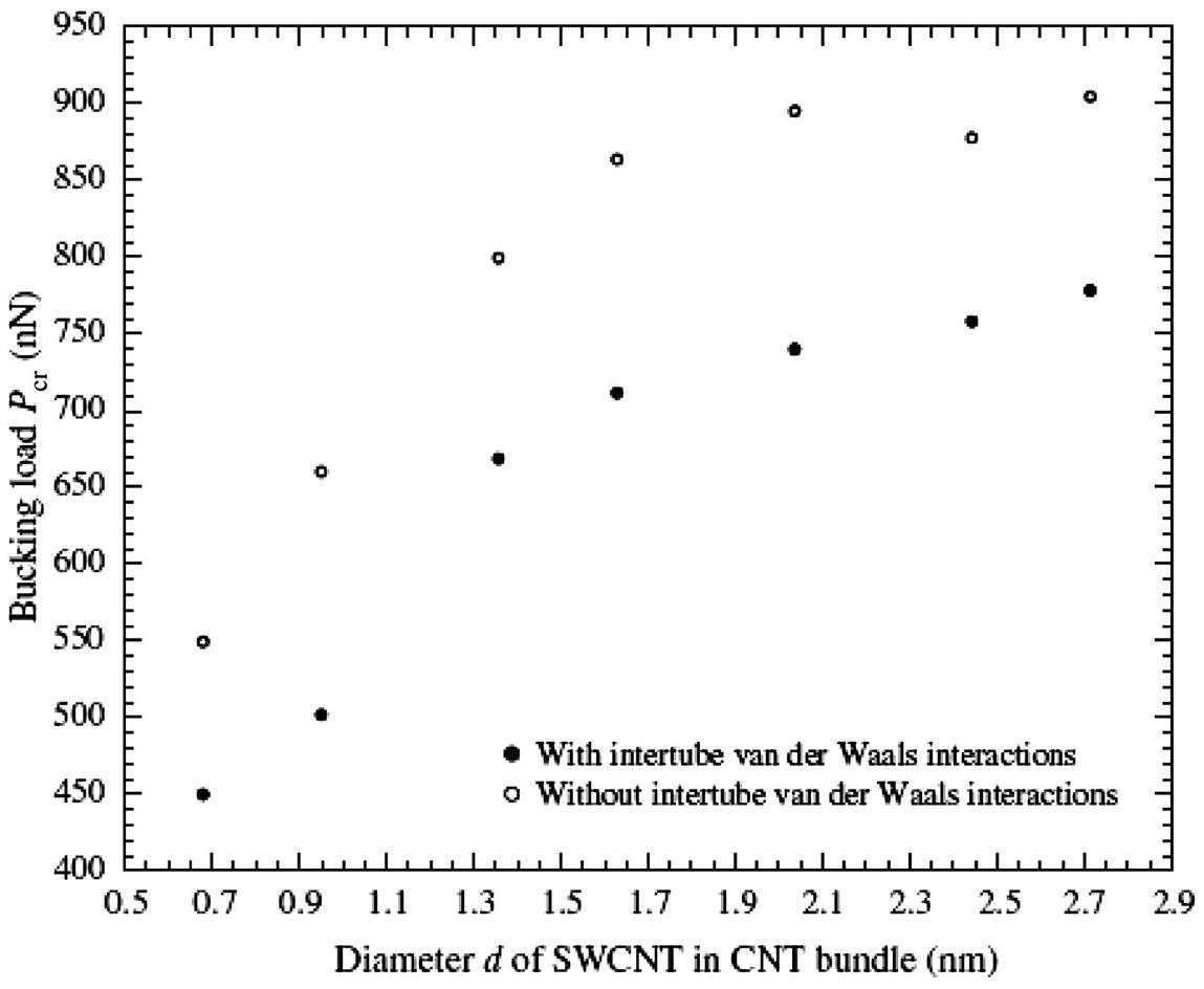
To understand how the intertube van der Waals interactions affect the compressive properties of CNT bundles, two sets of MD simulations were carried out: (1) with long-range intertube van der Waals interactions; and (2) without long-range intertube van der Waals interactions. It is noteworthy that intratube van der Waals interactions were omitted since they are not crucial to the calculations [15]. Fig. 3.43 depicts the buckling loads Pcr for the various sizes of CNT bundles, with (filled circles) and without (open circles) consideration of the intertube van der Waals interactions. From the plot, it is revealed that despite having the same number of SWCNTs in the bundles, the buckling loads Pcr will increase exponentially as the sizes of the individual SWCNTs in the CNT bundles increase. Even though the increasing trends of the buckling loads Pcr are similar, it is revealed that higher buckling loads Pcr can be achieved when the intertube van der Waals interactions were not considered. This is in agreement with the findings of Lu [42] who revealed that CNT bundles tend to have lower elastic moduli compared to individual SWCNT due to the weak intertube van der Waals interactions that make the CNT bundles weaker, since the individual SWCNTs can easily rotate and slide with respect to one another.
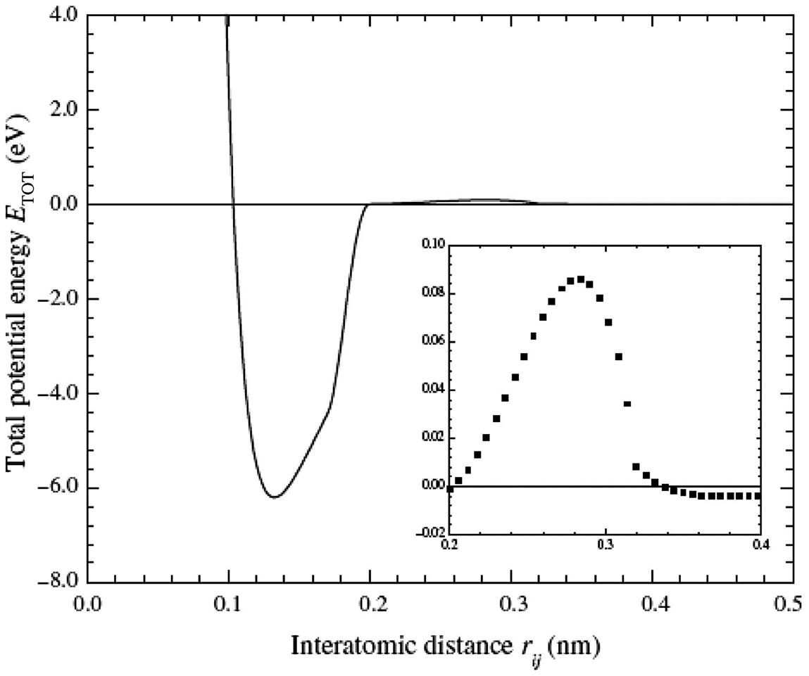
Apart from the above, similar MD simulations were performed at different interspacial gaps, where the long-range intertube van der Waals interactions can be found. This is to determine if the size of the interspacial gaps plays a role in the buckling properties of CNT bundles. In this work, a total of three interspacial gaps were used, i.e., 0.2, 0.34, and 0.51 nm. The interspacial gaps were not chosen smaller than 0.2 nm since according to Eq. (3.15), intertube covalent bonds will form when rij<0.2 nm. Fig. 3.44 shows the plot of buckling loads Pcr for different sizes of CNT bundles at various interspacial gaps. When the long-range intertube van der Waals interactions were not considered, the SWCNTs in the CNT bundles act as individual SWCNTs. The buckling loads Pcr for the different sizes of CNT bundles at different interspacial gaps are similar. They have an increasing exponential trend until the diameter d of the SWCNT in the CNT bundle reaches 2.04 nm, thereafter any further increase in diameter d will not result in any increase in its buckling load Pcr.
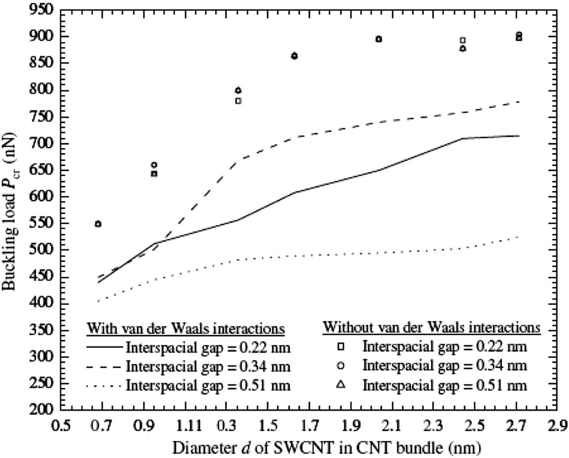
However, when the long-range intertube van der Waals interactions were considered in the computation, the buckling loads Pcr for the different sizes of CNT bundles were not the same. At an interspacial gap of 0.22 nm, the buckling load Pcr of the CNT bundle will be higher than that with an interspacial gap of 0.51 nm. This is due to the possibility of the formation of covalent bonds between individual SWCNTs when the CNT bundle is compressed, leading to a reduction in the interspacial gaps to less than 0.2 nm. Additionally, stronger intertube van der Waals interactions will be present than for a CNT bundle with an interspacial gap of 0.51 nm. The repulsive long-range intertube van der Waals interactions in the CNT bundle with an interspacial gap of 0.22 nm also explains why it has a lower buckling load Pcr than a CNT bundle with an interspacial gap of 0.34 nm (see inset of Fig. 3.45).
 rij<0.4 nm [15].
The critical strains ![]() of the various CNT bundles were also investigated. Fig. 3.46 shows that, in general, as the diameters d of the SWCNTs in the CNT bundle increase, the critical strain
of the various CNT bundles were also investigated. Fig. 3.46 shows that, in general, as the diameters d of the SWCNTs in the CNT bundle increase, the critical strain ![]() will decrease. Furthermore, the critical strains
will decrease. Furthermore, the critical strains ![]() of CNT bundles of seven SWCNTs is generally higher than that of CNT bundles of three SWCNTs. For example, the critical strain
of CNT bundles of seven SWCNTs is generally higher than that of CNT bundles of three SWCNTs. For example, the critical strain ![]() of the CNT bundle of seven (10, 10) SWCNTs is
of the CNT bundle of seven (10, 10) SWCNTs is ![]() =0.05010, while the critical strain
=0.05010, while the critical strain ![]() of the CNT bundle of three (10, 10) SWCNTs is lower at
of the CNT bundle of three (10, 10) SWCNTs is lower at ![]() =0.04435. This is due to the existence of more SWCNTs in the CNT bundle of seven which gives rise to higher strength and thus higher resistance to buckling. However, as the diameter d increases, the difference between the critical strains
=0.04435. This is due to the existence of more SWCNTs in the CNT bundle of seven which gives rise to higher strength and thus higher resistance to buckling. However, as the diameter d increases, the difference between the critical strains ![]() of both the CNT bundles of seven and three SWCNTs becomes smaller.
of both the CNT bundles of seven and three SWCNTs becomes smaller.

 of various sizes of CNT bundles of three and seven [15].
3.5.3 Twisting Effects of CNTs Bundles
MD simulations were performed on twisted CNT bundles, which comprise seven (5, 5) SWCNTs that are spaced 0.34 nm apart, under axial compression and tension. A twisting load was applied to six of the (5, 5) SWCNTs that surround a core SWCNT to form a twisted CNT bundle. A schematic cross-sectional view of the CNT bundle under study, which comprises six (5, 5) SWCNTs that surround a core (5, 5) SWCNT, is shown in Fig. 3.47.

The SWCNTs in the CNT bundle are spaced 0.34 nm apart, and the length of the bundle is lt=12.3 nm. The diameter of each (5, 5) SWCNT is dt=0.68 nm, and each CNT bundle contains 7000 atoms. A twisting load is applied to the six SWCNTs that surround core SWCNT. The twist angle ![]() is quantified as the relative twist between the two ends of the CNT bundle. A total of eight cases with different twisting angles
is quantified as the relative twist between the two ends of the CNT bundle. A total of eight cases with different twisting angles ![]() of 0, 15, 30, 60, 75, 90, 100, and 120 degrees were studied.
of 0, 15, 30, 60, 75, 90, 100, and 120 degrees were studied.
MD simulations were carried out on twisted CNT bundles under axial compressive and tensile forces. The axial compressive and tensile loads were achieved by applying a rate of 50 and 20 m/s, respectively, to both ends of the CNT bundles. The atoms at both ends of the CNT bundles were made transparent to the interatomic forces and were then moved either inwardly (compression) or outwardly (tension) along the axis in small steps followed by a conjugate gradient minimization method while the end atoms were kept fixed.
When the six surrounding SWCNTs were twisted, the overall lengths of these SWCNTs were maintained at 12.3 nm. As a result, the atoms in these SWCNTs move further apart from one another, stretching the C–C bonds between them. This effect is nevertheless insignificant as depicted in Fig. 3.48, which shows the average binding energy per atom of a surrounding SWCNT twisted at different angles ![]() . The plot shows that as the twist angle
. The plot shows that as the twist angle ![]() increases, the average binding energy per atom becomes weaker because the atoms are shifted further apart from one another. Despite the extension of the C–C bond lengths, the maximum difference in the average binding energy per atom when compared to a nontwisted SWCNT is only about 0.6%. This difference is small and is hence considered to be negligible in this study.
increases, the average binding energy per atom becomes weaker because the atoms are shifted further apart from one another. Despite the extension of the C–C bond lengths, the maximum difference in the average binding energy per atom when compared to a nontwisted SWCNT is only about 0.6%. This difference is small and is hence considered to be negligible in this study.

 [100].
3.5.3.1 Twisted CNT bundles under axial compression
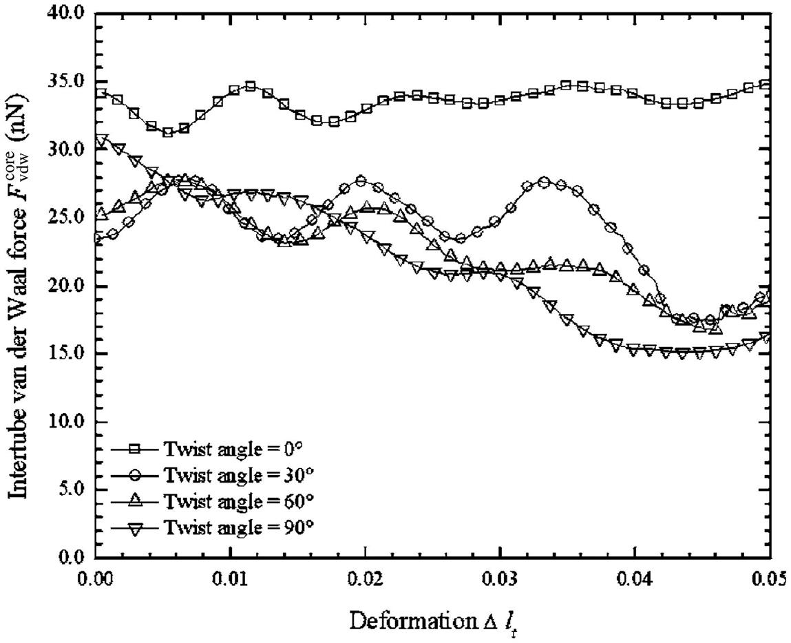
When a twisted CNT bundle is under axial compression, the six surrounding SWCNTs will expand and contract radially around the midlength along the center axis of the CNT bundle. To quantify the radial expansions and contractions and the morphological changes of the CNT bundle, the total intertube van der Waals force acting on the core SWCNT (![]() ) of each CNT bundle twisted at various angles (i.e.,
) of each CNT bundle twisted at various angles (i.e., ![]() =0, 30, 60, and 90 degrees) and its deformation
=0, 30, 60, and 90 degrees) and its deformation ![]() (i.e., defined as
(i.e., defined as ![]() =(lt−l)/lt, where l is the current length of the CNT bundle), were computed and plotted in Fig. 3.49. The graph shows that
=(lt−l)/lt, where l is the current length of the CNT bundle), were computed and plotted in Fig. 3.49. The graph shows that ![]() undergoes a cyclic pattern during compression. When the six surrounding SWCNTs expand radially,
undergoes a cyclic pattern during compression. When the six surrounding SWCNTs expand radially, ![]() becomes weaker as shown by the “valleys” of the plots in Fig. 3.49. However, when the six surrounding SWCNTs contract radially,
becomes weaker as shown by the “valleys” of the plots in Fig. 3.49. However, when the six surrounding SWCNTs contract radially, ![]() grows stronger, as shown by the “peaks” of the plots in Fig. 3.49.
grows stronger, as shown by the “peaks” of the plots in Fig. 3.49.
 ) of CNT bundles twisted at various angles during axial compression [100].
A twisted CNT bundle is expected to have a lower critical buckling load Pcr and critical strain ![]() than a nontwisted CNT bundle due to the curved geometries of the six surrounding SWCNTs that are formed by the twisting. Fig. 3.50 depicts the plot of the critical buckling load Pcr against the angle of twist
than a nontwisted CNT bundle due to the curved geometries of the six surrounding SWCNTs that are formed by the twisting. Fig. 3.50 depicts the plot of the critical buckling load Pcr against the angle of twist ![]() in the CNT bundle. As the twist angle
in the CNT bundle. As the twist angle ![]() increases from 0 to 60 degrees, the critical buckling load Pcr decreases by about 5% from 325 to 308 nN. A further increase in the twist angle
increases from 0 to 60 degrees, the critical buckling load Pcr decreases by about 5% from 325 to 308 nN. A further increase in the twist angle ![]() from 60 to 120 degrees, however, results in a larger drop of about 42% in the critical buckling load Pcr from 325 to 188 nN. This is because as the twist angle
from 60 to 120 degrees, however, results in a larger drop of about 42% in the critical buckling load Pcr from 325 to 188 nN. This is because as the twist angle ![]() grows, the compressive force at each end of the surrounding SWNCT becomes more misaligned, which causes the surrounding SWNCT to buckle more easily and at a lower load Pcr.
grows, the compressive force at each end of the surrounding SWNCT becomes more misaligned, which causes the surrounding SWNCT to buckle more easily and at a lower load Pcr.
 [100].
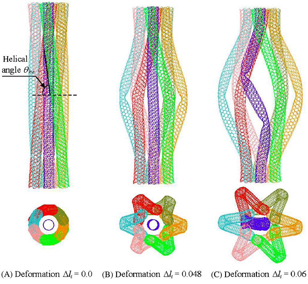
Additionally, it is also interesting to note that the six surrounding SWCNTs will buckle earlier than the core SWCNT due to their curved geometries. Fig. 3.51 shows the morphological changes of a 60 degree-twisted CNT bundle at different deformations ![]() . In the initial stage when
. In the initial stage when ![]() =0, the whole CNT bundle is relaxed, and the helical angle
=0, the whole CNT bundle is relaxed, and the helical angle ![]() that is formed due to the twisting of the six surrounding SWCNTs is about 77 degrees. Upon further compression, up to when the deformation
that is formed due to the twisting of the six surrounding SWCNTs is about 77 degrees. Upon further compression, up to when the deformation ![]() =0.048 (see Fig. 3.51B), the six surrounding SWCNTs buckle outwards from the center axis fractionally earlier and form a “bird-cage” pattern, while the core SWCNT remains unbuckled. The fully buckled CNT at
=0.048 (see Fig. 3.51B), the six surrounding SWCNTs buckle outwards from the center axis fractionally earlier and form a “bird-cage” pattern, while the core SWCNT remains unbuckled. The fully buckled CNT at ![]() =0.06 is shown in Fig. 3.51C.
=0.06 is shown in Fig. 3.51C.
 [100].
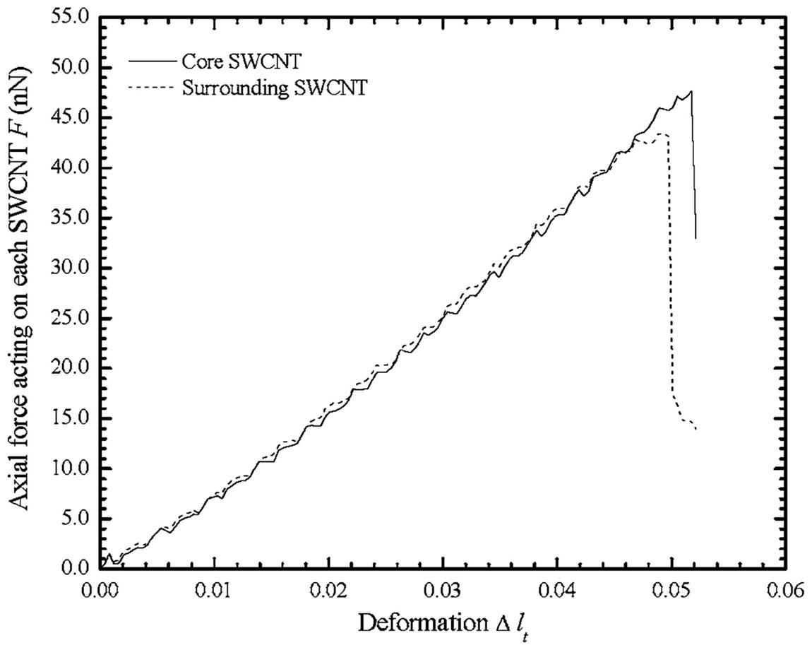
To gain further insight into the axial load P that each SWCNT experiences in the twisted CNT bundle during compressive loading, the axial force F of each individual SWCNT in the CNT bundle is plotted against its deformation ![]() as in Fig. 3.52. As the axial force F that acts on the six surrounding SWCNTs is the same, therefore only the axial force F that acts on one surrounding SWCNT and the core SWCNT is plotted. It is evident from the plot that the surrounding SWCNT buckles slightly earlier than the core SWCNT and at a lower critical buckling load Pcr. This is because since the surrounding SWCNT is geometrically twisted, therefore it is more susceptible to buckling than the core SWCNT.
as in Fig. 3.52. As the axial force F that acts on the six surrounding SWCNTs is the same, therefore only the axial force F that acts on one surrounding SWCNT and the core SWCNT is plotted. It is evident from the plot that the surrounding SWCNT buckles slightly earlier than the core SWCNT and at a lower critical buckling load Pcr. This is because since the surrounding SWCNT is geometrically twisted, therefore it is more susceptible to buckling than the core SWCNT.
3.5.3.2 Twisted CNT bundles under axial tension
In contrast to wire ropes, which provide better structural reliability and are mainly used in applications in which the tensile load is dominant, twisted CNT bundles tend to underperform when compared with nontwisted CNT bundles subjected to an axial tensile load. As a result of the twisting, the six surrounding SWCNTs are brought closer to each other under a helical angle, and junctions are formed between the neighboring SWCNTs. During axial tensile loading, the six surrounding SWCNTs were pulled even closer to the core SWCNT, which induced a reduction in the intertube distance din between individual SWCNTs. The plot in Fig. 3.53 shows the relationship between the intertube distance din and strain ![]() , which is computed as
, which is computed as ![]() =(l−lt)/lt, where l and lt are the current and initial length of the CNT bundle, respectively. From the plot, it is evident that the intertube distance din decreases as the strain
=(l−lt)/lt, where l and lt are the current and initial length of the CNT bundle, respectively. From the plot, it is evident that the intertube distance din decreases as the strain ![]() increases for CNT bundles with a large twist angle
increases for CNT bundles with a large twist angle ![]() . This is because when the six surrounding SWCNTs are twisted at a larger angle
. This is because when the six surrounding SWCNTs are twisted at a larger angle ![]() , they are more closely intertwined and are geometrically curved more prominently. Consequently when a tensile load is applied to both ends of the CNT bundles, the curved geometry of each of the six individual surrounding SWCNTs tends to straighten out, which leads to a reduction in the intertube distance din.
, they are more closely intertwined and are geometrically curved more prominently. Consequently when a tensile load is applied to both ends of the CNT bundles, the curved geometry of each of the six individual surrounding SWCNTs tends to straighten out, which leads to a reduction in the intertube distance din.
 at different strains [100].
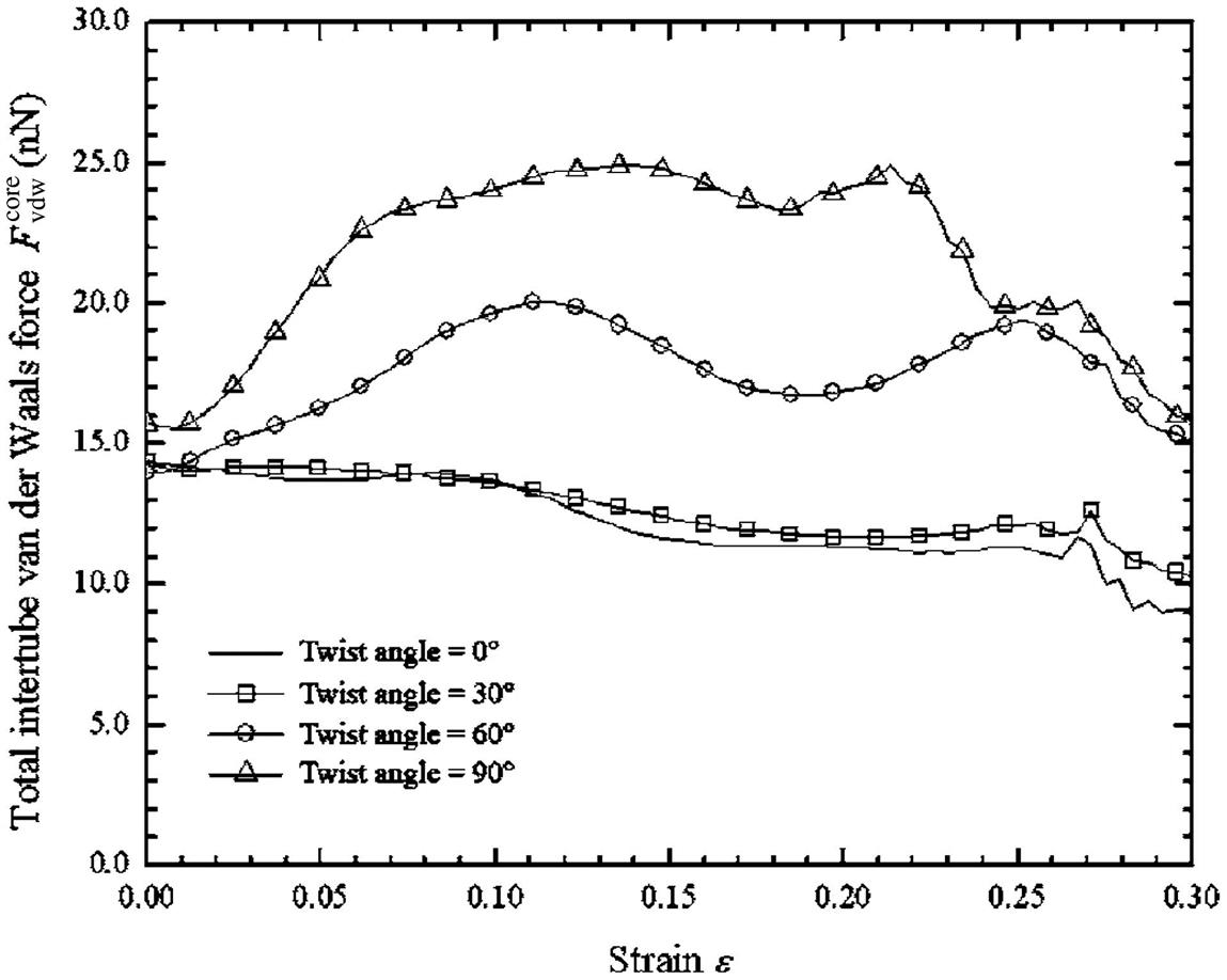
This phenomenon can also be confirmed by the plot of ![]() (total intertube van der Waals force
(total intertube van der Waals force ![]() acting on the core SWCNT) at different strains
acting on the core SWCNT) at different strains ![]() , as shown in Fig. 3.54. When a tensile load is applied to the CNT bundle,
, as shown in Fig. 3.54. When a tensile load is applied to the CNT bundle, ![]() increases until it reaches a maximum value. This indicates a decrease in the intertube distance din between the surrounding six SWCNTs and the core SWCNT.
increases until it reaches a maximum value. This indicates a decrease in the intertube distance din between the surrounding six SWCNTs and the core SWCNT. ![]() then slowly decreases, which is not a result of an increase in the intertube distance between the six surrounding SWCNTs and the core SWCNT, but is an indication of an increase in the repulsive energy, which is explained further below.
then slowly decreases, which is not a result of an increase in the intertube distance between the six surrounding SWCNTs and the core SWCNT, but is an indication of an increase in the repulsive energy, which is explained further below.
 ) of each CNT bundle (twisted at angles =0, 30, 60, and 90 degrees) during axial tension [100].
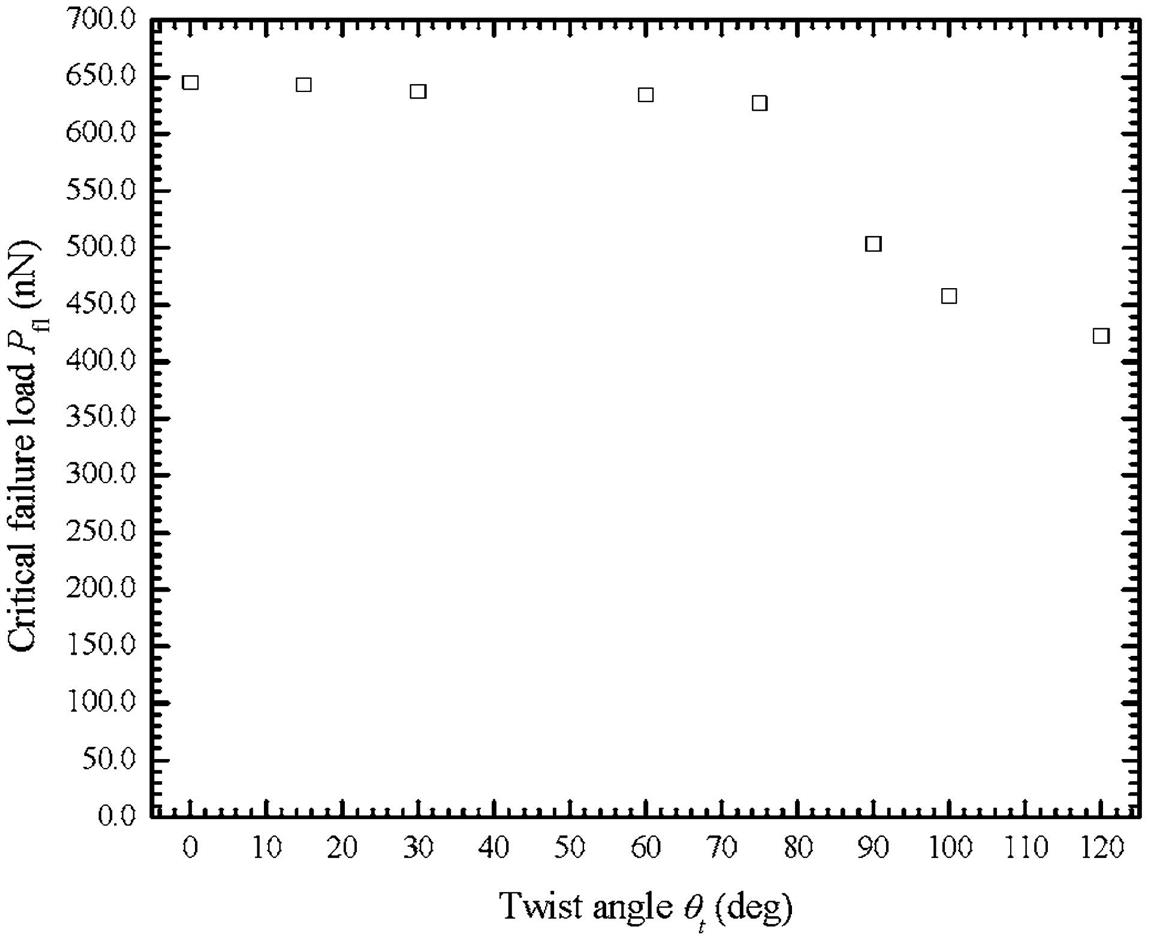
In contrast to the theory of wire ropes in a continuum domain, twisted CNT bundles do not exhibit better tensile properties, as shown in Fig. 3.55. When the twisting angle ![]() is greater than 75 degrees, the failure load Pfl decreases sharply. An investigation into the cause of this was carried out, and it was found that when a CNT bundle with a twisting angle
is greater than 75 degrees, the failure load Pfl decreases sharply. An investigation into the cause of this was carried out, and it was found that when a CNT bundle with a twisting angle ![]() that is greater than 75 degrees is subjected to axial tension, the intertube distance din between the seven SWCNTs decreases to less than 0.2 nm. This results in an increase in the repulsive energy between the seven SWCNTs since the contact distance is less than 0.34 nm. Consequently, these CNT bundles tend to fail at the junctions at lower loads and strains. This is in qualitative agreement with previous work [89–92], in which it was found that the dangling C–C bonds that were formed between SWCNTs and which were brought close together were not strong enough to withstand bending and axial forces.
that is greater than 75 degrees is subjected to axial tension, the intertube distance din between the seven SWCNTs decreases to less than 0.2 nm. This results in an increase in the repulsive energy between the seven SWCNTs since the contact distance is less than 0.34 nm. Consequently, these CNT bundles tend to fail at the junctions at lower loads and strains. This is in qualitative agreement with previous work [89–92], in which it was found that the dangling C–C bonds that were formed between SWCNTs and which were brought close together were not strong enough to withstand bending and axial forces.
 due to axial tensile force [100].
The total intertube van der Waals force ![]() and intertube repulsive force
and intertube repulsive force ![]() around the midlength of the CNTs that has been twisted at 0 and 90 degrees were extracted from the MD simulations and are depicted in Figs. 3.56 and 3.57, respectively. The midlength of the CNT bundle was chosen for the depictions, as this is where pairs of the twisted surrounding SWCNTs meet each other at a helical angle and form a junction where they overlap. As the strain
around the midlength of the CNTs that has been twisted at 0 and 90 degrees were extracted from the MD simulations and are depicted in Figs. 3.56 and 3.57, respectively. The midlength of the CNT bundle was chosen for the depictions, as this is where pairs of the twisted surrounding SWCNTs meet each other at a helical angle and form a junction where they overlap. As the strain ![]() becomes larger,
becomes larger, ![]() in the 90 degree-twisted CNT bundle increases due to the decreasing of intertube distance din (see Fig. 3.53). However,
in the 90 degree-twisted CNT bundle increases due to the decreasing of intertube distance din (see Fig. 3.53). However, ![]() in the nontwisted CNT bundle weakens steadily as the strain
in the nontwisted CNT bundle weakens steadily as the strain ![]() increases due to the elongation of the CNT bundle during tension, as there is no change in the intertube distance din.
increases due to the elongation of the CNT bundle during tension, as there is no change in the intertube distance din.

 around the midlength of CNT bundles twisted at 0 and 90 degrees [100].
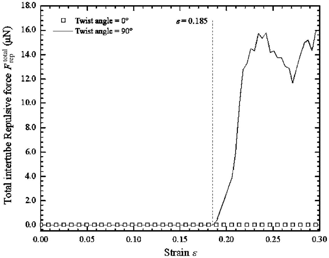
 around the midlength of a nontwisted CNT bundle and a 90 degree-twisted CNT bundle [100].
Throughout the whole tensile process, the nontwisted CNT bundle has no ![]() (intertube repulsive force) due to the large intertube spacing din, as shown in Fig. 3.57. Likewise, there is no
(intertube repulsive force) due to the large intertube spacing din, as shown in Fig. 3.57. Likewise, there is no ![]() present in the 90 degree-twisted CNT bundle that is twisted at 90 degrees up to
present in the 90 degree-twisted CNT bundle that is twisted at 90 degrees up to ![]() =0.185. This is because prior to
=0.185. This is because prior to ![]() =0.185, the intertube distance din is greater than 0.2 nm, and, according to Eq. (3.15), the repulsive force Frep is only computed when the distance between two atoms is less than 0.2 nm. However, after
=0.185, the intertube distance din is greater than 0.2 nm, and, according to Eq. (3.15), the repulsive force Frep is only computed when the distance between two atoms is less than 0.2 nm. However, after ![]() >0.185, the intertube distance din for the 90 degree-twisted CNT bundle reduces to less than 0.2 nm (see Fig. 3.53), which results in a sudden increase in
>0.185, the intertube distance din for the 90 degree-twisted CNT bundle reduces to less than 0.2 nm (see Fig. 3.53), which results in a sudden increase in ![]() and a decrease in
and a decrease in ![]() (total intertube van der Waals force), as shown in Fig. 3.56. It is worth noting that
(total intertube van der Waals force), as shown in Fig. 3.56. It is worth noting that ![]() and
and ![]() act radially on neighboring SWCNTs. As a result of the sudden surge in
act radially on neighboring SWCNTs. As a result of the sudden surge in ![]() , the 90 degree-twisted CNT bundle is weakened severely, and therefore only a low tensile load is needed to damage it. The damage often occurs at the junction areas (see Fig. 3.58).
, the 90 degree-twisted CNT bundle is weakened severely, and therefore only a low tensile load is needed to damage it. The damage often occurs at the junction areas (see Fig. 3.58).
 =0, where the intertube distance din is about 0.32 nm; (B) strain =0.24, where the intertube distance din is about 0.19 nm. The junction area at which the two SWCNTs overlap is shown in black. The double-headed arrows represent the intertube repulsive force Frep [100].
As a consequence of the sudden increase in ![]() at the junction areas at which the individual SWCNTs overlap, CNT bundles that are twisted at an angle
at the junction areas at which the individual SWCNTs overlap, CNT bundles that are twisted at an angle ![]() >75 degrees will collapse at lower critical strains
>75 degrees will collapse at lower critical strains ![]() , as shown in Fig. 3.59. The plot shows that the critical strains remain at around
, as shown in Fig. 3.59. The plot shows that the critical strains remain at around ![]() 0.35 up to a twisting angle
0.35 up to a twisting angle ![]() of 75 degrees, and decrease significantly thereafter to
of 75 degrees, and decrease significantly thereafter to ![]() 0.18.
0.18.
 of CNT bundles twisted at different angles due to axial tensile force [100].
Fig. 3.60 shows the cross-sectional view of two CNT bundles with a twisting angle of 0 and 120 degrees, respectively, at different strains. It is evident from this figure that the 120 degree-twisted CNT bundle suffers from a large amount of distortion of the individual SWCNTs compared with the nontwisted CNT bundle. The SWCNTs in the 120 degree-twisted CNT bundle lose their cylindrical shapes at high strains, which results in a dislocation of the hexagonal arrangement of the C atoms. The distortion of individual SWCNTs in the CNT bundle is manifested by the compressive van der Waals force FvdW and the repulsive force Frep between the seven SWCNTs.
 [100].
3.6 Fracture of CNTs
Usually, Young’s modulus is assumed to be constant. It can be determined from the second derivative of potential function by fitting the potential energy into a cubic polynomial function. For CNTs, Young’s modulus is dependent on strain and treated as constant if the strain is small. In general, we can obtain the derivative of a potential function in a smooth stress–strain curve in the elastic region, but not for the elasto-plastic-failure region. This is due to large fluctuation of stresses. Thus it is difficult to determine some mechanical properties, such as the tensile strength, elastic strain limit, maximum strain, by fitting the potential energy into a smooth stress–strain curve.
In order to describe the complete stress–strain relationship from the elastic deformation to rapture, the stress–strain curves of single and multiwalled CNTs under tension deformation are obtained in our simulations by applying a rate of 20 m/s to both ends. The atoms at the end of the CNTs are then moved outwardly along the axis by small steps, followed by a conjugate gradient minimization method while keeping them fixed in plane.
In the microcanonical ensemble MD simulations of the CNTs, the strain is computed by ![]() in which L0 and L being the initial and current length of the CNTs, respectively, and the stress is given by
in which L0 and L being the initial and current length of the CNTs, respectively, and the stress is given by ![]() . The axial force F is obtained by summing the interatomic force for the atoms at the end of CNTs and the cross-sectional area is
. The axial force F is obtained by summing the interatomic force for the atoms at the end of CNTs and the cross-sectional area is ![]() , where d is the diameter of the CNT and h the thickness of the CNT that is taken as
, where d is the diameter of the CNT and h the thickness of the CNT that is taken as ![]() nm for (10, 10) single-walled CNT,
nm for (10, 10) single-walled CNT, ![]() nm for (5, 5) and (10, 10) two-walled CNT,
nm for (5, 5) and (10, 10) two-walled CNT, ![]() nm for (5, 5), (10, 10), and (15, 15) three-walled CNT, and
nm for (5, 5), (10, 10), and (15, 15) three-walled CNT, and ![]() nm for (5, 5), (10, 10), (15, 15), and (20, 20) four-walled CNT.
nm for (5, 5), (10, 10), (15, 15), and (20, 20) four-walled CNT.
In order to validate the present MD simulation, the stress–strain responses are determined for a (12, 12) single-walled CNT with a length-to-diameter ratio ![]() . Our MD simulation is first compared with the results of Belytschko et al. [64] as depicted in Fig. 3.61. It is observed that our stress–strain curve deviates slightly from the results in [64]; nevertheless, they are in reasonable agreement. In the second comparison study listed in Table 3.17, our MD simulations of Young’s modulus of various single-walled CNTs are in close agreement with the ab initio results of Kudin et al. [93]. With the above comparison studies, we therefore confirm the accuracy of our MD simulation.
. Our MD simulation is first compared with the results of Belytschko et al. [64] as depicted in Fig. 3.61. It is observed that our stress–strain curve deviates slightly from the results in [64]; nevertheless, they are in reasonable agreement. In the second comparison study listed in Table 3.17, our MD simulations of Young’s modulus of various single-walled CNTs are in close agreement with the ab initio results of Kudin et al. [93]. With the above comparison studies, we therefore confirm the accuracy of our MD simulation.

Table 3.17
Young’s Modulus of Various CNTs Computed by MD (This Work) and Ab Initio Simulations [13]
| CNT | Young’s Modulus | |
| MD | Ab Initio [93] | |
| (4, 4) | 55.3 | 56.4 |
| (7, 0) | 55.7 | 56.3 |
| (7, 7) | 56.0 | 56.5 |
| (12, 0) | 56.4 | 55.2 |

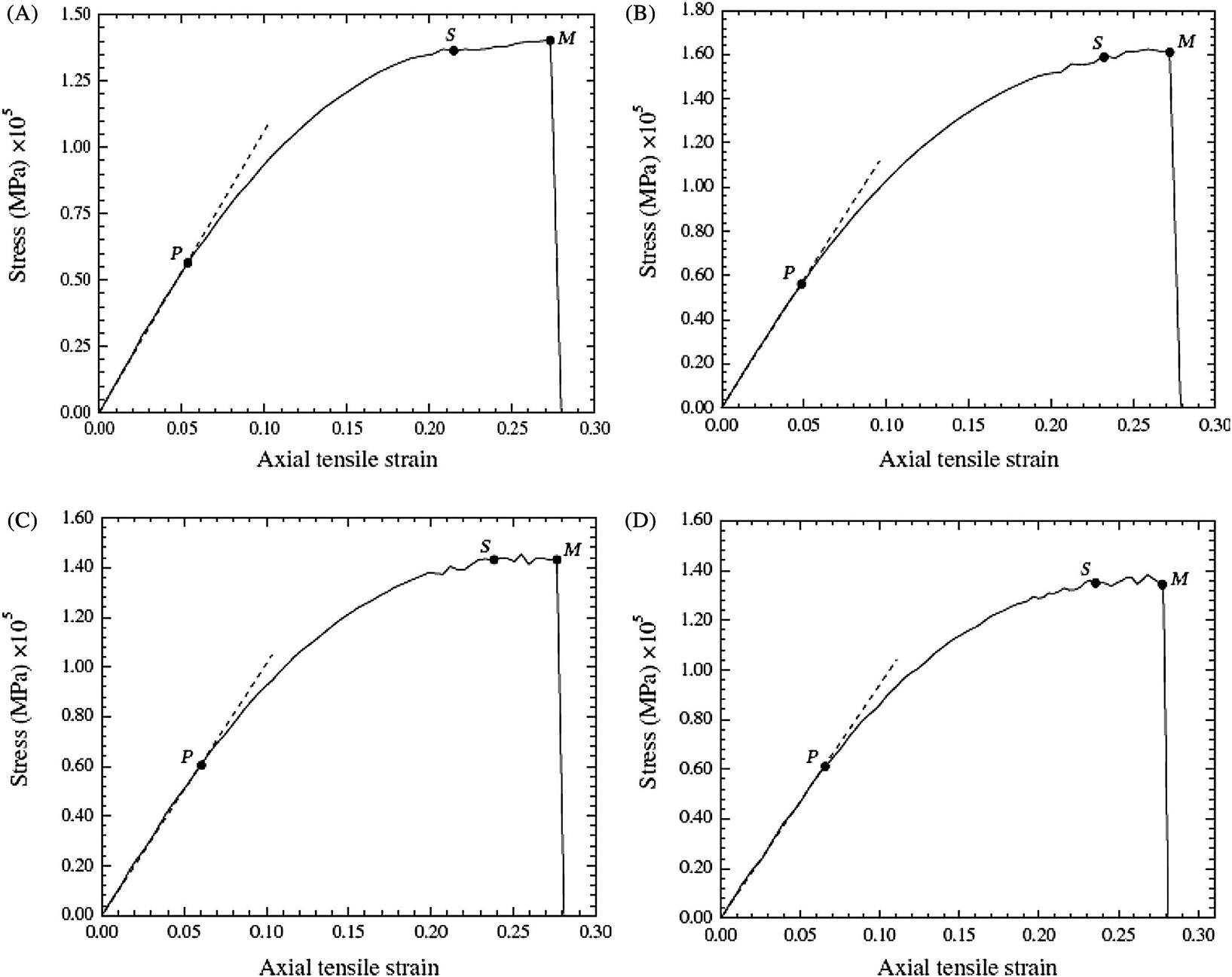
The elastoplastic responses of the CNTs are simulated and plotted in Fig. 3.62A–H for the length-to-diameter ratio of 4.5 and 9.1. It is evident that when ![]() , the stress–strain relationship follows the Hooke’s law, i.e.,
, the stress–strain relationship follows the Hooke’s law, i.e., ![]() . Here,
. Here, ![]() corresponds to point P in Fig. 3.62A–H, and is the proportional strain limit. It is observed that as the strain increases, the stress–strain curve behaves nonlinearly with a decreasing gradient until it reaches the yield strain
corresponds to point P in Fig. 3.62A–H, and is the proportional strain limit. It is observed that as the strain increases, the stress–strain curve behaves nonlinearly with a decreasing gradient until it reaches the yield strain ![]() , which corresponds to yield point S in Fig. 3.62A–H. Using the regression analysis, the stress–strain curve is represented by
, which corresponds to yield point S in Fig. 3.62A–H. Using the regression analysis, the stress–strain curve is represented by ![]() where
where ![]() . The values of A and B are determined by fitting the stress–strain relationship to a smooth curve again using the regression analysis, as shown in Table 3.18 for various CNTs. At the yield point, we have
. The values of A and B are determined by fitting the stress–strain relationship to a smooth curve again using the regression analysis, as shown in Table 3.18 for various CNTs. At the yield point, we have ![]() , and thus the yield strain limit
, and thus the yield strain limit ![]() becomes
becomes ![]() . Beyond the yield point S, considerable plastic deformation occurs without a noticeable increase in the stress; at the strain limit of
. Beyond the yield point S, considerable plastic deformation occurs without a noticeable increase in the stress; at the strain limit of ![]() , the stress can be approximately expressed as
, the stress can be approximately expressed as ![]() . This ductile behavior can be observed in our animated MD simulations, showing wave propagation from the center to the two ends of the CNTs and then back to the center. This phenomenon of wave propagation displays the rearrangement of configuration of the CNTs for strain release via the formation of the Stone–Wales defects.
. This ductile behavior can be observed in our animated MD simulations, showing wave propagation from the center to the two ends of the CNTs and then back to the center. This phenomenon of wave propagation displays the rearrangement of configuration of the CNTs for strain release via the formation of the Stone–Wales defects.
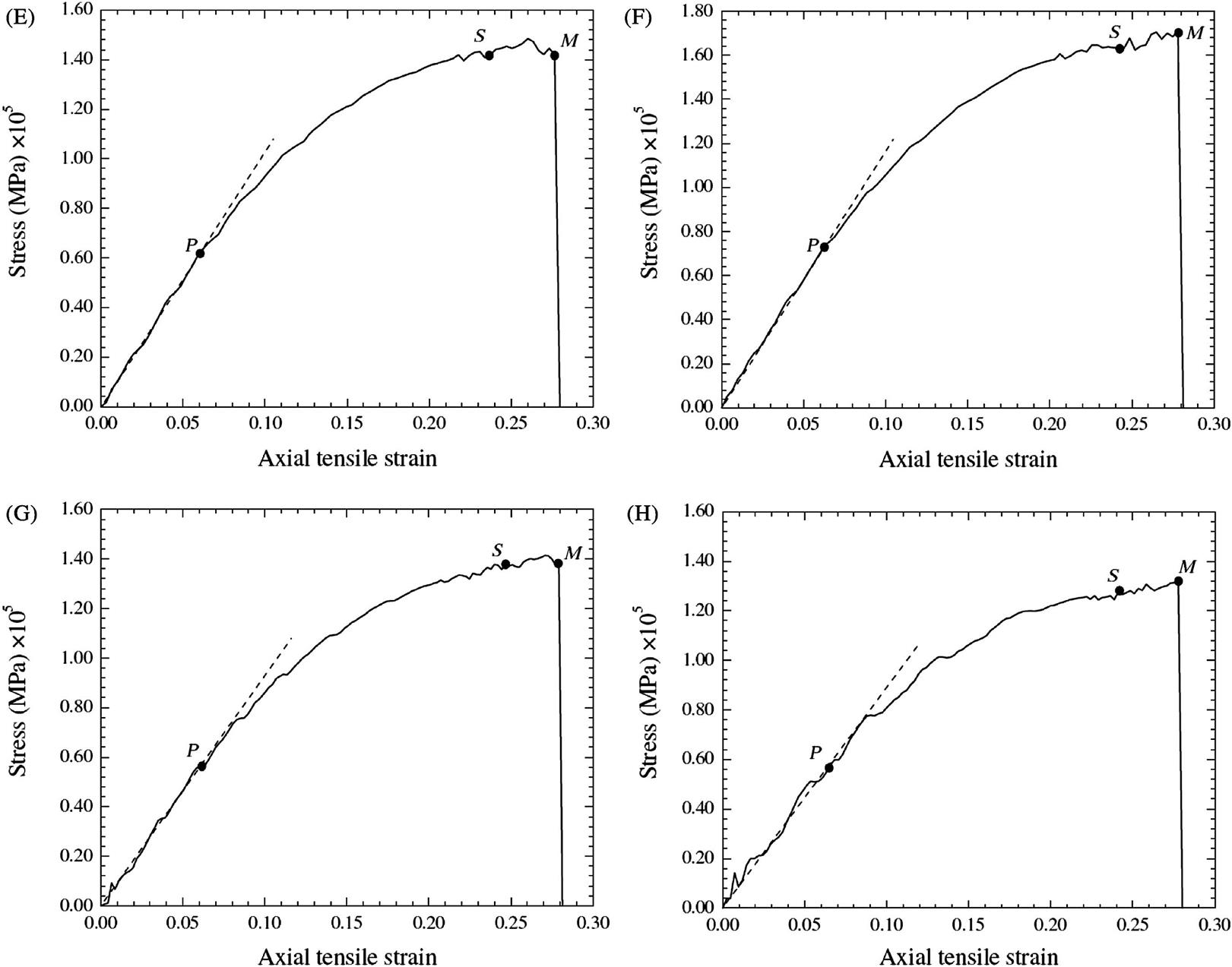
 . (B) The transverse elastic–plastic response of a two-walled (5, 5) and (10, 10) CNT under axial tension with . (C) The transverse elastic–plastic response of a three-walled (5, 5), (10, 10), and (15, 15) CNT under axial tension with . (D) The transverse elastic–plastic response of a four-walled (5, 5), (10, 10), (15, 15), and (20, 20) CNT under axial tension with . (E) The transverse elastic–plastic response of a single-walled CNT (10, 10) under axial tension with
  . (F) The transverse elastic–plastic response of a two-walled (5, 5) and (10, 10) CNT under axial tension with . (G) The transverse elastic–plastic response of a three-walled (5, 5), (10, 10), and (15, 15) CNT under axial tension with . (H) The transverse elastic–plastic response of a four-walled (5, 5), (10, 10), (15, 15), and (20, 20) CNT under axial tension with [13].
Table 3.18
Material Properties of Selected Single and Multiwalled CNTs [13]
| L/D | Young’s Modulus (TPa) | A (TPa) | B (TPa) | Proportional Strength (MPa) | Yield Strength (MPa) | Tensile Strength (MPa) | Proportional Strain Limit | Elastic Strain Limit | Maximum Strain | |
| Single-walled CNT of (10, 10) | 4.5 | 1.043 | −2.625 | 1.211 | 6.103×10⁴ | 1.369×10⁵ | 1.404×10⁵ | 0.0585 | 0.231 | 0.280 |
| 9.1 | 1.031 | −2.522 | 1.190 | 6.271×10⁴ | 1.421×10⁵ | 1.485×10⁵ | 0.0594 | 0.236 | 0.279 | |
| Two-walled CNT of (5, 5) and (10, 10) | 4.5 | 1.161 | −2.543 | 1.259 | 7.231×10⁴ | 1.614×10⁵ | 1.624×10⁵ | 0.0627 | 0.247 | 0.279 |
| 9.1 | 1.175 | −2.810 | 1.362 | 7.287×10⁴ | 1.633×10⁵ | 1.684×10⁵ | 0.0621 | 0.242 | 0.281 | |
| Three-walled CNT of (5, 5), (10, 10) and (15, 15) | 4.5 | 1.000 | −2.358 | 1.160 | 6.068×10⁴ | 1.430×10⁵ | 1.434×10⁵ | 0.0605 | 0.238 | 0.281 |
| 9.1 | 0.972 | −2.275 | 1.120 | 5.645×10⁴ | 1.381×10⁵ | 1.414×10⁵ | 0.0611 | 0.246 | 0.282 | |
| Four-walled CNT of (5, 5), (10, 10), (15, 15) and (20, 20) | 4.5 | 0.932 | −2.234 | 1.103 | 6.075×10⁴ | 1.343×10⁵ | 1.382×10⁵ | 0.0654 | 0.235 | 0.281 |
| 9.1 | 0.872 | −2.132 | 1.023 | 5.784×10⁴ | 1.278×10⁵ | 1.327×10⁵ | 0.0633 | 0.241 | 0.280 |

Table 3.18 lists the computed Young’s modulus, Poisson’s ratio, yield strength, tensile strength, elastic strain limit, and maximum strain for selected single to four-walled armchair CNTs with the length-to-diameter ratios of the CNTs equal to 4.5 and 9.1. It is observed that the properties are dependent on the number of layers of the CNT. Nevertheless, there are small differences in the properties of CNTs for the length-to-diameter ratios of 4.5 and 9.1. It is evident that the effect of geometrical size on the mechanical properties of CNTs is relatively small and, with the same number of layers, we find that the mechanical properties of CNTs can be treated as the same for all length-to-diameter ratios.
Fig. 3.63 shows the formation of (5–77–5) defects due to a 90 degrees rotation of a bond during the plastic deformation. The initial (5–77–5) defect is formed at a strain of 24%. As the strain increases, more (5–77–5) defects are generated along the circumferential direction, as shown in Fig. 3.63. When the strain reaches the maximum strain point M at 0.256, two bonds are broken leading to two holes, as shown in Fig. 3.64. This observation is in close agreement with the quantum mechanical simulated results of Dumitrica et al. [94], which showed that failures occurred at strain above 0.240 for armchair CNTs. As the strain increases, more bonds are broken and the holes become larger until the CNT fractures. The brittle fracture process is displayed in Fig. 3.64A–D for the outermost layer of the four-walled CNT. Upon reaching the maximum strain ![]() , the CNTs rupture very quickly and completely fracture within a small period of time, which is displayed in Fig. 3.62A–H. Fig. 3.65 shows the entire failure process of the four-walled CNT of (5, 5), (10, 10), (15, 15), and (20, 20). When strain is at 0.263, bond breaking initially takes place at the outermost layer (first layer) with all the other three layers remaining undamaged. The phenomenon whereby the outermost layer of multiwalled CNT is first damaged is consistent with the experimental result of Yu et al. [95]. As the strain increases to 0.268, the outermost layer is almost totally fractured, while one bond in the second layer begins to break, and the third and innermost layers remain undamaged. However, a bond is observed to have broken in the third layer as the strain increases to 0.275. At this time, the third layer starts fracturing, even though no bond breaking is found in the innermost layer (fourth layer). When strain is at 0.279, a bond starts to break in the innermost layer and the three outer layers are all completely damaged. Eventually, the entire four-walled CNT disintegrates when the strain is at 0.28. The above exemplifies that multiwalled CNTs can sustain elongations up to 28%, which is in good agreement with the experimental result of Bozovic et al. [96].
, the CNTs rupture very quickly and completely fracture within a small period of time, which is displayed in Fig. 3.62A–H. Fig. 3.65 shows the entire failure process of the four-walled CNT of (5, 5), (10, 10), (15, 15), and (20, 20). When strain is at 0.263, bond breaking initially takes place at the outermost layer (first layer) with all the other three layers remaining undamaged. The phenomenon whereby the outermost layer of multiwalled CNT is first damaged is consistent with the experimental result of Yu et al. [95]. As the strain increases to 0.268, the outermost layer is almost totally fractured, while one bond in the second layer begins to break, and the third and innermost layers remain undamaged. However, a bond is observed to have broken in the third layer as the strain increases to 0.275. At this time, the third layer starts fracturing, even though no bond breaking is found in the innermost layer (fourth layer). When strain is at 0.279, a bond starts to break in the innermost layer and the three outer layers are all completely damaged. Eventually, the entire four-walled CNT disintegrates when the strain is at 0.28. The above exemplifies that multiwalled CNTs can sustain elongations up to 28%, which is in good agreement with the experimental result of Bozovic et al. [96].

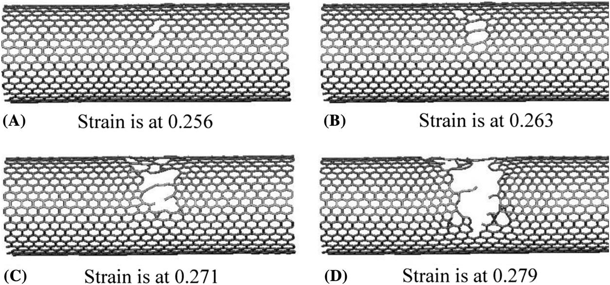
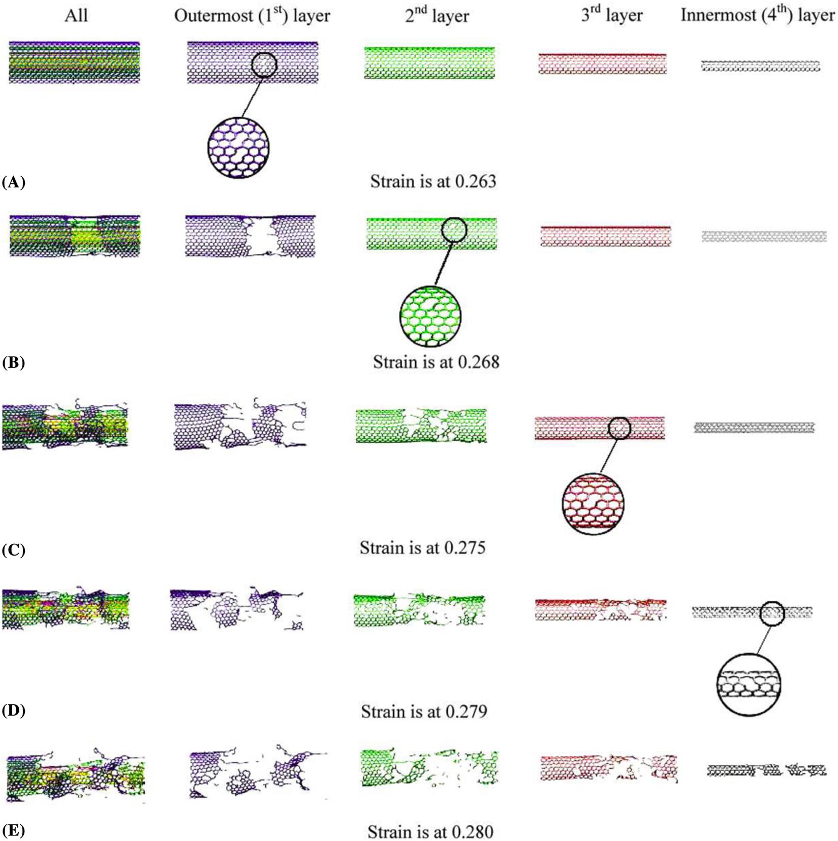 . (A) Bond breaking first takes place in the outermost layer when the strain is at 0.263. (B) The second layer starts to break when the strain is at 0.268. (C) The third layer starts to break when the strain is at 0.275. (D) The innermost layer starts to break when the strain is at 0.279. (E) The entire four-walled CNT completely fractures when the strain is at 0.280 [13].
3.7 Thermal Stability of CNTs
To study how the atomic structures of CNTs change and their stability at various temperatures, we have incorporated the Berendsen thermostat [97] into the MD simulation. This method requires the CNT to be coupled to an external heat bath, which is fixed at a desired temperature. The bath acts as a source of thermal energy, supplying or removing heat from the CNT as appropriate. The velocities of the atoms are scaled at each time-step, such that the rate of temperature change is proportional to the difference in temperature between the bath and the CNT
(3.24)
where ![]() is the coupling parameter whose magnitude determines how tightly the bath and the CNT are coupled together. A larger
is the coupling parameter whose magnitude determines how tightly the bath and the CNT are coupled together. A larger ![]() will give a weaker coupling, while a smaller
will give a weaker coupling, while a smaller ![]() will give a stronger coupling. This method gives an exponential decay/growth of the system toward the desired temperature. The change in temperature between successive time-steps is
will give a stronger coupling. This method gives an exponential decay/growth of the system toward the desired temperature. The change in temperature between successive time-steps is
(3.25)
and therefore, the scaling factor ![]() for the velocities is
for the velocities is
(3.26)
From Eq. (3.26), it can be seen that if the coupling parameter ![]() equals to the time-step
equals to the time-step ![]() , then the Berendsen scheme is equivalent to the simple ad hoc velocity scaling method. A coupling constant
, then the Berendsen scheme is equivalent to the simple ad hoc velocity scaling method. A coupling constant ![]() of approximately 0.4 ps has been suggested [97] as a suitable value to use when the time-step is 1 fs, thereby giving
of approximately 0.4 ps has been suggested [97] as a suitable value to use when the time-step is 1 fs, thereby giving ![]() 0.0025.
0.0025.
To apply the Berendsen thermostat [97] to the study of CNTs, the atoms are first given random initial velocities from a uniform velocity distribution on an interval [−1, +1]. These velocities are scaled so that the total linear momentum is zero. Therefore,
(3.27)
where ![]() represents the x, y, and z directions. These velocities are then rescaled to achieve the desired temperature T by using the scaling factor in Eq. (3.26) for all directions.
represents the x, y, and z directions. These velocities are then rescaled to achieve the desired temperature T by using the scaling factor in Eq. (3.26) for all directions.
From these initially assigned velocities, the Maxwell velocity distribution should develop during equilibration. The Maxwell–Boltzmann law [98] is used to evaluate the Maxwell velocity distribution analytically, and is defined as
(3.28)
which measures the fraction of N atoms having velocities within an interval dv of a particular value v. From Eq. (3.28), the Maxwell velocity distribution can then be evaluated analytically as
(3.29)
The distribution is Gaussian with standard deviation ![]() about the mean value
about the mean value ![]() =0. Fig. 3.66 shows the Maxwell velocity distribution of a (10, 10) single-walled CNT exposed to various temperatures T at 100K, 200K, 300K, and 400K employing the Berendsen thermostat [97]. As the temperature T increases, the standard deviation
=0. Fig. 3.66 shows the Maxwell velocity distribution of a (10, 10) single-walled CNT exposed to various temperatures T at 100K, 200K, 300K, and 400K employing the Berendsen thermostat [97]. As the temperature T increases, the standard deviation ![]() approaches to uniformity.
approaches to uniformity.
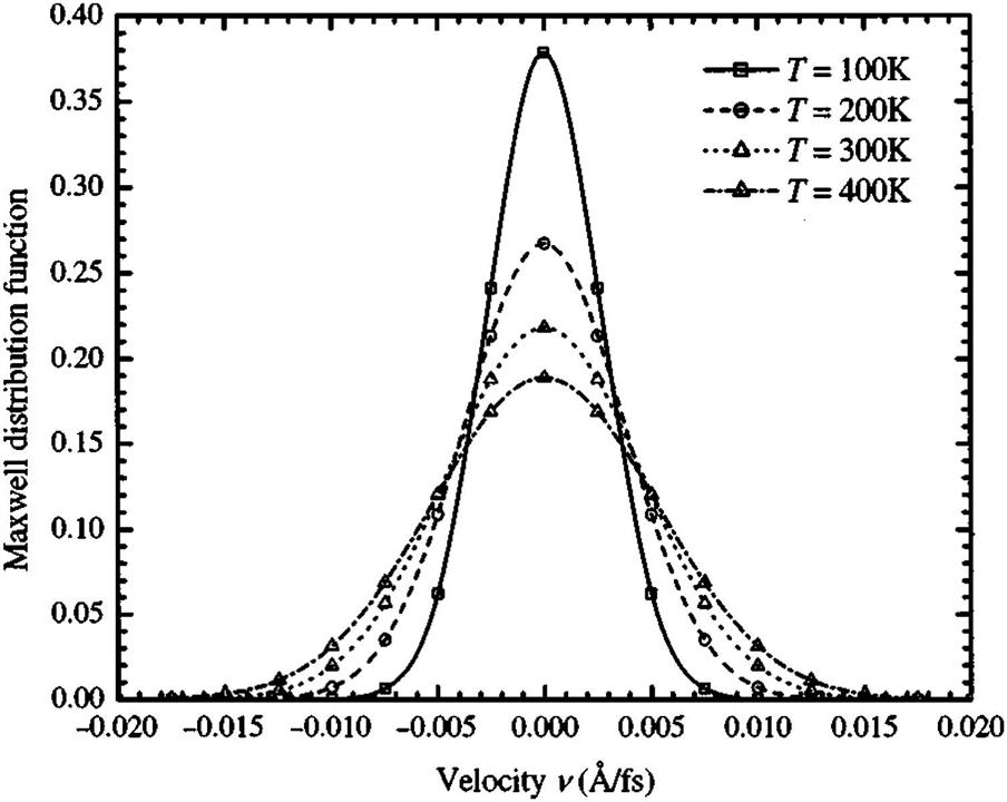
To verify if the Maxwell velocity distribution has developed, the velocity distribution ![]() is time averaged over a number of time-steps and compared to the Maxwell velocity distribution at the same kinetic energy. Fig. 3.67 shows the comparison of the (10, 10) single-walled CNT at temperature T=300K. The plot shows good agreement and signifies that an equilibration state is achieved.
is time averaged over a number of time-steps and compared to the Maxwell velocity distribution at the same kinetic energy. Fig. 3.67 shows the comparison of the (10, 10) single-walled CNT at temperature T=300K. The plot shows good agreement and signifies that an equilibration state is achieved.
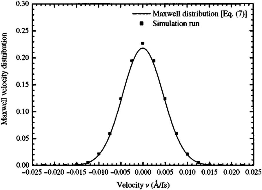
During the simulation, it is instructive to follow the development of the Maxwell distribution and, hence the approach to equilibrium, by monitoring the time behavior of the kinetic portion of Boltzmann’s celebrated H-function [98] expressed as
(3.30)
Fig. 3.68 shows the instantaneous H-function computed during the equilibration of the (10, 10) single-walled CNT at temperature T=300K. In the figure, the horizontal line at H=−0.00505 is the value of the H-function for the Maxwell velocity distribution at the kinetic energy of the simulation. After about 3000 time-steps, the instantaneous H-function converges to the Maxwell’s value of the H-function, thus indicating that Maxwell distribution develops within about 3000 time-steps. Above 3000 time-steps, the instantaneous H-function fluctuates along the Maxwell’s value of the H-function, and hence the system is considered to be in equilibrium.

At equilibration, the potential energy EPOT and kinetic energy EK fluctuate about a steady value. Fig. 3.69 shows that the (10, 10) single-walled CNT achieves equilibration at temperature T=300K. The kinetic energy EK fluctuates around 9.0 eV, while the potential energy EPOT fluctuates around −7230 eV over 4000 time-steps. The plot also indicates the conservation of the total energy. During the simulation, the total energy ETOT has a maximum deviation of 0.033% from its average value of −7220.92 eV.
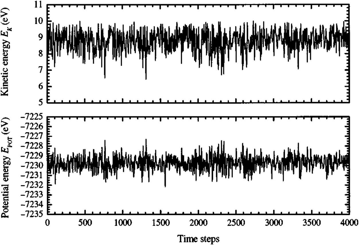
Both open-ended and close-capped single-walled CNTs are investigated to determine the influence of the caps on the CNTs. All the single-walled CNTs are made to adhere to the Maxwell velocity distribution and the H-function to confirm their equilibrium state.
3.7.1 Close-Capped Single-Walled CNTs
Three different lengths of (5, 5) close-capped single-walled CNTs are investigated. The lengths L are 122, 183, and 244 Å. Fig. 3.70 shows that a 122 Å-long (5, 5) close-capped single-walled CNT remains undeformed at temperatures T from 300K up to 2000K. At T=2000K, the close-capped single-walled CNT begins to deform slightly at its body and disintegrates completely at T=3489K.

A similar simulation is carried out on a 183 Å-long (5, 5) close-capped single-walled CNT as depicted in Fig. 3.71. The longer close-capped single-walled CNT begins to deform structurally at temperature T=2000K before breaking down completely at a lower temperature T=3333K.

Similarly atomic structural deformation is evident for the 244 Å-long (5, 5) close-capped single-walled CNT before collapsing at T=2946K.
3.7.2 Open-Ended Single-Walled CNTs
As a comparison to close-capped (5, 5) single-walled CNTs, different lengths (L=122, 183, and 244 Å) of open-ended (5, 5) single-walled CNTs are also investigated. The relaxed CNTs at various temperatures are shown in Figs. 3.72 and 3.73.


It can be seen in Fig. 3.72 that the ends of the 122 Å-long open-ended (5, 5) single-walled CNT begins to flange slightly at temperature T=300K. As the temperature increases to T=1000K, the open-ended (5, 5) single-walled CNT begins to deform structurally. And when the temperature increases to T=3000K, the CNT bends before disintegrating at T=3582K. The bending-induced thermal contraction causes the end-to-end distance to shrink, and agrees with the findings of Schelling et al. [99].
Deformation at the ends of the 183 Å-long open-ended (5, 5) single-walled CNT is apparent at temperature T=1000K, as shown in Fig. 3.73. The CNT starts to bend from T=2000–3000K, causing a reduction of the end-to-end distance. At T=3337K, the 183 Å-long open-ended (5, 5) single-walled CNT can no longer withstand the thermal load and disintegrates.
A 244 Å-long open-ended (5, 5) single-walled CNT is also modeled and simulated as thermal load is applied to it. The results show that it collapses after it reaches a temperature of T=2798K.
From Figs. 3.70–3.73, we can observe that the atomic structural deformation differs between close-capped and open-ended (5, 5) single-walled CNTs. For open-ended CNTs, the end atoms begin to deform first, probably due to unsatisfied bonds at the ends of the CNTs to satisfy their bonds with bonding to other carbon atoms, while the body of the close-capped CNTs deform first when subjected to thermal loads. However, the maximum critical temperatures both the open-ended and close-capped CNTs can withstand before breaking down are less than 5% different (see Fig. 3.74). Hence for the ease of modeling, further open-ended (10, 10) and (12, 12) single-walled CNTs are investigated.
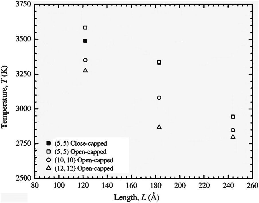
The response to temperature for the open-ended (10, 10) and (12, 12) single-walled CNT is included in Fig. 3.74. From the plots, all the single-walled CNTs tend to have lower thermal stability as their lengths L increase. For instance at length L=122 Å, the (10, 10) single-walled CNT can resist up to T=3350K before collapsing. However, the maximum temperature a 244 Å-long (10, 10) single-walled CNT can withstand is lower, i.e., T=2798K.
Additionally, as the diameter dt of the CNTs increases, its ability to withstand thermal loads is lower. This is exemplified by the maximum temperature T=2868K the (12, 12) single-walled CNT can withstand as compared to the lower maximum temperature T=3337K for the (5, 5) single-walled CNT when both lengths L=183 Å.
According to Fig. 3.74, it is evident that the length L of the single-walled CNT affects its response to temperature T. Fig. 3.75 explains the cause of this phenomena using the (10, 10) single-walled CNT as an example.

Comparing to the shorter (10, 10) single-walled CNT that is shown in Fig. 3.74, it can be deduced that longer single-walled CNTs tend to break down at a lower temperature than shorter single-walled CNTs at longer lengths. This can be explained by the plot in Fig. 3.75. Although both lengths of (10, 10) single-walled CNT have similar kinetic energy EK per atom at a certain temperature T, the potential energy EPOT per atom is different. The longer (10, 10) single-walled CNT has lower potential energy EPOT per atom compared to the shorter (10, 10) single-walled CNT at all temperatures T. When subjected to heat, the chemical bonds from the longer single-walled CNT break down more easily, because each atom from the longer (10, 10) single-walled CNT has lower potential energy EPOT. Consequently, the longer (10, 10) single-walled CNT collapses at a lower temperature T than the shorter (10, 10) single-walled CNT.
3.7.3 Open-Ended Multiwalled CNTs
The response of multiwalled CNTs with different geometries at different temperatures T are also investigated. In this study, two multiwalled CNTs, namely, the (5, 5) and (10, 10), and (10, 10) and (15, 15) multiwalled CNTs with the same lengths L=61.55 Å are considered. The relaxed multiwalled CNTs at various temperatures T are shown in Fig. 3.76 and 3.77. All of the multiwalled CNTs adhere to the Maxwell velocity distribution and the H-function to confirm their equilibrium state.


Fig. 3.76 depicts the morphological changes of the (5, 5) and (10, 10) multiwalled CNT when subjected to an increasing temperature T from 0K to 3000K. At T=300K, the multiwalled CNT is similar to that of an ideal structure. However, at T=1000K, both layers start to deform. Significant flanges at both ends of the outer layer of the multiwalled CNT are also observed, and the ends of the inner layer start to close together. Before the multiwalled CNT collapses after T=2000K, more deformation occurs at both layers. Due to the high temperature, the atoms at both layers vibrate more and collide with each other resulting in the disintegration of the multiwalled CNT.
When exposed to an increasing temperature T, the second (10, 10) and (15, 15) multiwalled CNT deforms as shown in Fig. 3.77. Like all of the multiwalled CNTs, the (10, 10) and (15, 15) multiwalled CNT maintains its overall geometry at T=300K. Flanges at both ends of the multiwalled CNT are formed at T=1000K until T=2300K, when the ends of both layers begin to close. On further increase of temperature T, the bonds break and the multiwalled CNT eventually collapses.