Atomic Finite Element Method and Coupling With Atomistic-Continuum Method
Abstract
This chapter presents a multiscale method by coupling the developed atomistic-continuum theory with an atomic finite element method. It takes advantage of both continuum and atomic simulations and is currently a popular technique in the modeling of large-scale nanostructures. The critical bending angle for buckling of (12, 12) carbon nanotube is 13 degrees in both coupling simulation and atomic finite element method, along with well-agreed energy change from the two methods both before and after the buckling occurs. In Chapter 4, Atomistic-Continuum Theory, the atomistic-continuum simulation presents very precise results prior to buckling but less precise results than those of atomic finite element method after buckling. Therefore, the present coupling simulation shows highly efficient performance for localized problems.
Keywords
Coupling simulation; atomic finite element method; highly efficient performance
5.1 Introduction
In this chapter, the multiscale coupling of the developed mesh-free computational scheme with an atomic simulation technique is investigated. The multiscale method takes advantage of both continuum and atomic simulations and is currently a popular technique in the modeling of large-scale nanostructures. In most multiscale studies, research is focused on the approach to bridging two different scales, and less attention is paid to the efficiency of continuum simulations. For example, continuum simulation based on the standard Cauchy–Born rule has been applied in multiscale analysis. The present study mainly investigates the application of the developed mesh-free method in multiscale analysis. A previous coupling technique, the bridging domain method, is employed to bridge two scales. Multiscale computational examples are tested, and good computational efficiency is obtained.
As illustrated in previous chapters, atom-based methods consume a huge amount of computational resources and are restricted to very small systems. Continuum modeling can significantly reduce the degrees of freedom of problems, and the theoretical analysis and numerical simulation of large-scale systems become possible. However, continuum simulations cannot completely substitute for the atom-based method since it they employ a homogenization technique. In particular, the continuum methods are unable to capture the microscale physical laws of nanostructures. Multiscale analysis is thus emerging as a feasible and efficient approach to large-size problems. The multiscale method couples continuum simulation and atomic simulation and makes use of both approaches. The basic idea of the multiscale method is to use atomic simulation for the localized region in which the discrete motion of atoms is important and to use the continuum method for the remaining regions in which the deformation is homogeneous and smooth. A key issue associated with the multiscale method is the way to bridge the two different scales smoothly. Currently, researchers have developed several techniques to couple the continuum and atomic methods. Here, three popular approaches, the quasicontinuum method [1–9], the bridging domain method [10–12], and the bridging scale method [13–17], are introduced. The bridging domain method is used in the present research.
5.2 Atomic Finite Element Method
The multiscale method requires an appropriate atomic simulation approach. An atomic simulation method that has the same solution framework as the present mesh-free method is introduced in this section. This atomic simulation method will be employed in the present multiscale computation. In the previous chapters, this method has been used in testing the efficiency and accuracy of the developed mesh-free method.
Let us consider a system that contains NA carbon atoms. The energy that is stored in the atomic bonds is a function of the positions of all atoms, as follows:
(5.1)
where ![]() is the position of atom I, and
is the position of atom I, and ![]() is the Brenner potential.
is the Brenner potential.
The total potential energy of the atomic system is
(5.2)
where ![]() , and
, and ![]() is the external force (if any) that is exerted on atom I. The state of the stable configuration corresponds to
is the external force (if any) that is exerted on atom I. The state of the stable configuration corresponds to
(5.3)
The Taylor expansion of ![]() around an initial guess of
around an initial guess of ![]() for the equilibrium state gives
for the equilibrium state gives
(5.4)
Its substitution into Eq. (5.3) yields the following governing equation for the displacement ![]() ,
,
(5.5)
where the stiffness matrix is
(5.6)
and the nonequilibrium force vector is
(5.7)
where ![]() is the external force vector. The equilibrium state is obtained by iteratively solving Eq. (5.5) until
is the external force vector. The equilibrium state is obtained by iteratively solving Eq. (5.5) until ![]() reaches zero.
reaches zero.
In [18,19], Liu et al. introduced the concept of the atomic-scale finite element to assemble the global stiffness matrix and force vector, and they employed finite element software to solve large-scale problems. In the present computation, all work, including assembling the stiffness matrix and force vector and solving the equation system, is performed with our Fortran codes. This atomic simulation approach has been used in previous chapters to test the efficiency of the continuum method. It is noted that the stiffness matrix ![]() lacks the positive definiteness beyond the buckling, and the method that is described in Chapter 4, Atomistic-Continuum Theory, should be used to ensure the convergence of the algorithm.
lacks the positive definiteness beyond the buckling, and the method that is described in Chapter 4, Atomistic-Continuum Theory, should be used to ensure the convergence of the algorithm.
5.3 Coupling of Atomic Finite Element Method With Atomistic-Continuum Method
5.3.1 Quasicontinuum Method
The quasicontinuum method was proposed by Tadmor et al. [2,3] for modeling 2-D crystallites, and it has been used to study a variety of fundamental aspects of deformation in crystalline solids, including fracture, grain boundary structure and deformation, nano-indentation, and 3-D dislocation junctions [1–9].
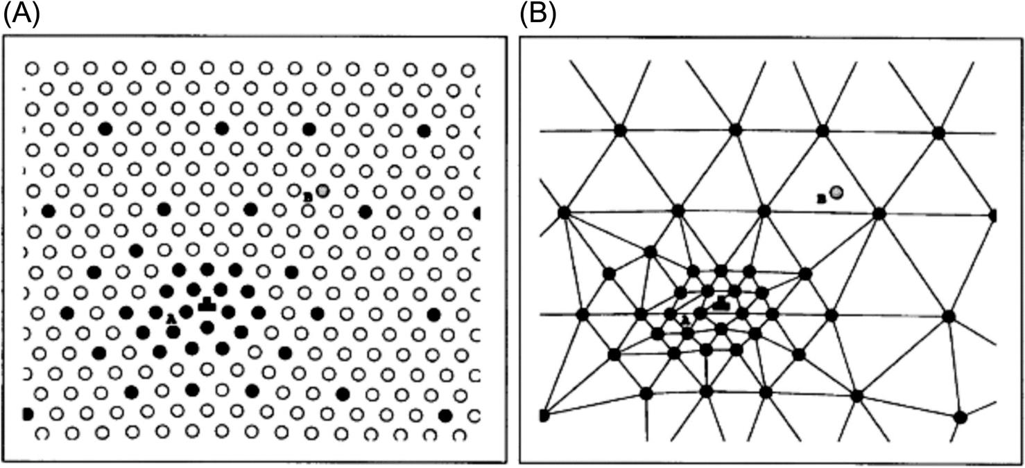
The quasicontinuum method introduced the concept of representative atoms. Shown in Fig. 5.1A is a crystalline solid that involves a Lomer dislocation [9]: the filled circles denote the chosen representative atoms. Around the core of the dislocation, the deformation is drastic, the microcosmic change of the atomic structure needs to be described and traced, and all atoms are chosen as the representative atoms. Far away from the core of the dislocation, the field is slowly varying and the deformation is homogeneous, and certain sparse atoms are chosen as the representative atoms. In the former region, the atoms are called nonlocal atoms, and their interactions with the neighboring atoms are reflected. The atoms in the latter region are called local atoms, and a continuum discretization scheme can be established based on them.
The total potential energy of the quasicontinuum model can be obtained as
(5.8)
The first and second terms in Eq. (5.8) denote the energies of the nonlocal and local atoms, respectively. ![]() is the weight function and refers to the number of atoms that this representative atom can represent. In practice, the local region can be discretized as a series of elements by using the representative atoms as nodes (see Fig. 5.1B).
is the weight function and refers to the number of atoms that this representative atom can represent. In practice, the local region can be discretized as a series of elements by using the representative atoms as nodes (see Fig. 5.1B).
In the quasicontinuum method, a ghost force often arises in the transition zone between the local and nonlocal regions, even when the crystal is undeformed. To avoid the effect of this ghost force, the energy is augmented by a term associated with the work done by the ghost force:
(5.9)
The ghost force ![]() is calculated each time the status of the representative atoms is updated and is held constant until an update is required due to the evolving state of the deformation [9].
is calculated each time the status of the representative atoms is updated and is held constant until an update is required due to the evolving state of the deformation [9].
5.3.2 Bridging Domain Method
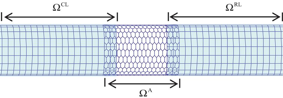
The bridging domain method was proposed by Belytschko and Xiao [10,11], was used to simulate the fracture of graphite sheets [10], and was recently extended to simulate the fracture of large-diameter carbon nanotubes (CNTs) [11,12]. In this technique, the entire domain is decomposed into three types of regions (see Fig. 5.2): an atomic region ![]() in which the atomic movement is described, a continuum region
in which the atomic movement is described, a continuum region ![]() in which the lattice undergoes a smooth deformation and the continuum simulation is used, and an overlapping region
in which the lattice undergoes a smooth deformation and the continuum simulation is used, and an overlapping region ![]() in which the atomic and continuum models overlap. In the atomic and continuum regions, the energy is computed using the atomic and continuum methods, respectively. In the overlapping region, the potential energy is expressed as a linear combination of the continuum and atomic energies. This ensures smooth bridging between the continuum and atomic deformation fields.
in which the atomic and continuum models overlap. In the atomic and continuum regions, the energy is computed using the atomic and continuum methods, respectively. In the overlapping region, the potential energy is expressed as a linear combination of the continuum and atomic energies. This ensures smooth bridging between the continuum and atomic deformation fields.
 and a full atomic region
  with an overlapping region
  [20].
[20].5.3.3 Bridging Scale Method
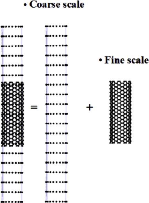
The bridging scale method was developed by Liu and his coworkers [13–17]. In this method, the total displacement field is decomposed into two different components, as follows:
(5.10)
where ![]() is the coarse scale component and can be established in a continuum discretization frame such as the finite element or mesh-free method.
is the coarse scale component and can be established in a continuum discretization frame such as the finite element or mesh-free method. ![]() is the fine scale component that must be determined by the atom-based method. Far away from the localized domain,
is the fine scale component that must be determined by the atom-based method. Far away from the localized domain, ![]() becomes insignificant, or, mathematically,
becomes insignificant, or, mathematically, ![]() has a vanishing projection onto the coarse scale basis function. Therefore, atomic simulation is only needed in the localized regions. Fig. 5.3 shows the computational scheme for the bridging scale method. There are two different computational domains. The first is the coupled domain in which the atomic structure coexists with the continuum discretization. The second domain is the coarse scale domain in which only the continuum discretization exists. The coarse and fine scale solutions are coupled. In the computation, the coarse scale solution is solved in the entire domain, whereas the fine scale solution is only solved in the localized region. Bridging between the coarse and fine scales is realized by transparently exchanging information between the coarse and fine scale regions.
has a vanishing projection onto the coarse scale basis function. Therefore, atomic simulation is only needed in the localized regions. Fig. 5.3 shows the computational scheme for the bridging scale method. There are two different computational domains. The first is the coupled domain in which the atomic structure coexists with the continuum discretization. The second domain is the coarse scale domain in which only the continuum discretization exists. The coarse and fine scale solutions are coupled. In the computation, the coarse scale solution is solved in the entire domain, whereas the fine scale solution is only solved in the localized region. Bridging between the coarse and fine scales is realized by transparently exchanging information between the coarse and fine scale regions.
The present multiscale computational scheme couples the developed mesh-free method and the atomic simulation method presented in Section 5.2. The coupling approach used is the bridging domain method. The main purpose is to investigate the validity of the developed mesh-free computational framework in the multiscale simulation.
Referring to Fig. 5.2, the entire domain is decomposed into three regions: ![]() ,
, ![]() , and
, and ![]() . The mesh-free method developed in Chapter 4, Atomistic-Continuum Theory, is used in the continuum region. As specified in Chapter 4, Atomistic-Continuum Theory, the mesh-free nodes are uniformly collocated along the axial and circumferential directions, and the background integral cells are in accordance with the nodal arrangements. The crossing points of the axial and circumferential lines denote the mesh-free nodes in Fig. 5.2.
. The mesh-free method developed in Chapter 4, Atomistic-Continuum Theory, is used in the continuum region. As specified in Chapter 4, Atomistic-Continuum Theory, the mesh-free nodes are uniformly collocated along the axial and circumferential directions, and the background integral cells are in accordance with the nodal arrangements. The crossing points of the axial and circumferential lines denote the mesh-free nodes in Fig. 5.2.
The total energy of the coupled system can be written as a weighted sum of energies for the continuum and atomic regions:
(5.11)
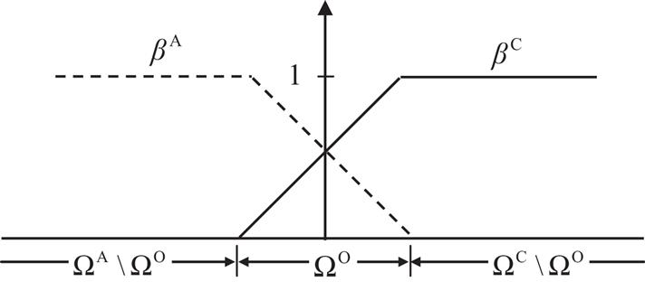
where ![]() is the position of atom I in the undeformed single-walled CNT (SWCNT), and the weight functions
is the position of atom I in the undeformed single-walled CNT (SWCNT), and the weight functions ![]() and
and ![]() take the forms [10–12]:
take the forms [10–12]:
(5.12)
 (5.12)
where the symbol “” denotes the set-minus operation, and the parameter α varies linearly from 0 to 1 across the overlapping region, as shown in Fig. 5.4. This method thus allows the minimization of the continuum and atomic configurations concurrently, and the two scale solutions can simultaneously be solved.


The total potential energy of the coupled system is
(5.13)
The nonequilibrium force vector and stiffness matrix can be obtained by
(5.14)
(5.15)
In [10–12], the augmented Lagrange multiplier method was used to ensure that the continuum displacements conformed to the atomic displacements at the discrete positions of the atoms in the overlapping region. In the present research, the atomic displacement in the overlapping region is directly interpolated with the mesh-free nodal parameters at each iterative step, which means that the vector ![]() contains all of the mesh-free modal parameters, but only the current positions of the atoms outside the overlapping region. The stable configuration can be obtained by iteratively solving
contains all of the mesh-free modal parameters, but only the current positions of the atoms outside the overlapping region. The stable configuration can be obtained by iteratively solving ![]() until
until ![]() reaches zero. Moreover, the treatment described in Section 4.5.8 is also effective for the present problem.
reaches zero. Moreover, the treatment described in Section 4.5.8 is also effective for the present problem.
5.4 Tensile Failure
Two examples are chosen to test the application of the mesh-free method in multiscale analysis and illustrate the validity of the present multiscale computational scheme. The first example is the bending test, for which the Brenner potential with the second set of parameters is used. The second example considers the fracture of SWCNTs with a single-atom vacancy. As described before, the Brenner potential always results in overestimated fracture stress. Therefore, the modified second-generation Brenner potential is used for the second example.
5.4.1 Bending Test
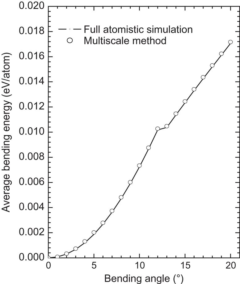
A (12, 12) SWCNT is chosen upon which to perform the bending test. The SWCNT has 42 hexagonal cells (a total of 2040 atoms) in its length. Atomic simulation is used for the middle portion, whereas the left and right parts are modeled using a mesh-free method in which 396 mesh-free nodes are used. In the overlapping region, the atomic position is interpolated using the mesh-free nodes, and the pure atomic region contains 552 atoms. The degrees of freedom of the system are reduced from 3×2024 to 3×948. The bending deformation is imposed using the mode II loading method described in Chapter 4, Atomistic-Continuum Theory. For each loading step, the tube is bent by 1 degree per loading step. Fig. 5.5 shows a plot of the changes in the average energy per atom against the bending angle for the multiscale simulation and the full atomic simulation. Buckling occurs at a bending angle of 13 degrees in both simulations, and the energy change from the two methods also agrees quite well both before and after the buckling occurs. Fig. 5.6 shows the deformations at a bending angle of 20 degrees, and a comparison of the two methods reveals that a precise simulation can be achieved with the multiscale method. In Chapter 4, Atomistic-Continuum Theory, the mesh-free simulation presents very precise results prior to buckling, but after buckling, the results are less precise than those of the full atomic simulation. The present multiscale simulation presents good agreement with the atomic simulation before and after buckling, which shows that the multiscale method is very efficient for localized problems.

5.4.2 Tensile Failure of SWCNTs With a Single-Atom Vacancy Defect
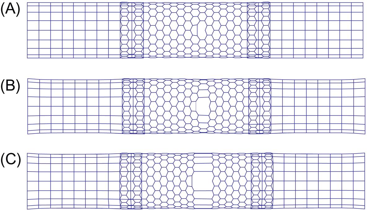
In this example, the multiscale method is used to study the tensile failure of an SWCNT with a single-atom vacancy defect. This kind of defect has a significant effect on the strength of a CNT and thus has attracted considerable research attention. In the computation, one atom is removed from the hexagonal network in the atomic region, which leads to the reconstruction of the atomic structure near the vacancy in the initial equilibrium configuration [12]. Here, this initial equilibrium configuration is determined with the full atomic simulation before the multiscale computation is performed. The SWCNT is stretched until the fracture occurs. Fig. 5.7 shows the stress–strain curves for (18, 0) and (12, 12) SWCNTs. The tensile force can be computed by summing the nodal force along the end of the CNT, and the stress is calculated by dividing the tensile force by the cross-sectional area ![]() . Fig. 5.8 shows the cracking procedure for an (18, 0) SWCNT, with Fig. 5.8A showing the initial equilibrium configuration of the undeformed SWCNT, Fig. 5.8B highlighting the breakage of the bonds around the defect, and Fig. 5.8C displaying the completely fractured SWCNT in which all of the bonds around the circumference have failed. Fig. 5.9 shows the fracture progression for a (12, 12) SWCNT, from which it can be seen that the failure path displays a slight difference from that of the (18, 0) SWCNT. In the present simulation, the failure is actually a brittle fracture. To show the cracking progression, a larger positive number β is added to the diagonal elements of the stiffness matrix after the occurrence of the fracture.
. Fig. 5.8 shows the cracking procedure for an (18, 0) SWCNT, with Fig. 5.8A showing the initial equilibrium configuration of the undeformed SWCNT, Fig. 5.8B highlighting the breakage of the bonds around the defect, and Fig. 5.8C displaying the completely fractured SWCNT in which all of the bonds around the circumference have failed. Fig. 5.9 shows the fracture progression for a (12, 12) SWCNT, from which it can be seen that the failure path displays a slight difference from that of the (18, 0) SWCNT. In the present simulation, the failure is actually a brittle fracture. To show the cracking progression, a larger positive number β is added to the diagonal elements of the stiffness matrix after the occurrence of the fracture.