6 Dual-Energy CT Imaging with Fast-kVp Switching

Dual-energy CT is an imaging technique that has been known and extensively studied for many decades [1–8]. However, due to various technical challenges, only recently has dual-energy CT imaging become a reality. Recent advances in CT scanner technologies have generated a renewed interest in dual-energy CT [9–14], which has led to the commercialization of dual-energy CT systems available for routine clinical use [10,12–14].

Dual-energy CT is a special CT imaging procedure in which two CT scans of a patient are acquired in different x-ray tube potentials (and spectra) and used to perform energy- and material-selective reconstruction of the patient. Relative to conventional single-energy (SE) CT imaging, dual-energy CT imaging offers the capability to enhance material differentiation and reduce beam-hardening artifacts.

Figure 6.1a shows a routine abdominal SE CT exam, and Figure 6.1b and c shows a corresponding dual-energy CT exam. Dual-energy CT enables the separation of kidney stone (calcium) from iodine-based intravenous contrast by decomposing the dual-energy data into iodine (atomic number of 53) and water (effective atomic number of 7.42). Furthermore, the reduction of beam-hardening artifacts near the kidney stones (circled) is readily apparent by comparing Figure 6.1a and b.

Images

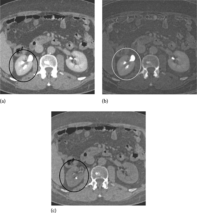
FIGURE 6.1
A comparison between a post-contrast SE abdomen CT exam and dual-energy CT exam of the same patient. (a) SE exam at 120 kVp. (b,c) Dual-energy exam using 140 and 80 kVp enables the separation of kidney stone (calcium) from iodine-based intravenous contrast by decomposing the dual-energy data into iodine (left) and water (right) material pairs. The reduction of beam-hardening artifacts near the kidney stones (circled) is readily apparent by comparing (a) and (b). (Image courtesy of Dr. Amy Hara, Mayo Clinic, Scottsdale, AZ.)

Dual-energy CT imaging has the potential to improve the efficacy of many clinical applications including abdomen [15], neurology [16], pulmonary embolism [17], and bone mineral densitometry [3]. Investigators have begun to establish the clinical efficacy of dual-energy CT for plaque characterization [18].

Conventional dual-energy CT exam is accomplished by the so-called “rotate–rotate” technique: first a low-kVp CT exam is acquired, and then the patient is translated back to the origin, followed by the acquisition of a high-kVp CT exam. Similar to digital subtraction angiograph (DSA), this technique is very sensitive to patient motion because the time interval between the two kVps is in the order of seconds. As a result, poor spatial–temporal registration between high- and low-kVp x-ray beams is a major source of image artifacts in conventional dual-energy CT imaging. Compared to SE CT, motion-induced artifacts, such as blurring of the edges and streaks centered on objects that are moving, are more severe in dual-energy CT. Furthermore, patient motion can be falsely interpreted as a change in tissue composition, which, typically manifested as light-and-dark edge effect around the moving objects, can cause inaccurate material densities and/or misdiagnosis (Figure 6.2).

To address the motion issue, a fast-kVp switching (FKS) dual-energy CT imaging method, where kVp is rapidly switched between low and high kVp in adjacent views, has recently been proposed [12–14]. Compared to conventional dual-energy CT imaging, FKS dual-energy CT imaging has several benefits including precise temporal and spatial view registration, helical and axial acquisitions, and full field of view. It also presents several design challenges that warrant careful considerations.

Images

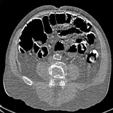
FIGURE 6.2
Patient motion is a major source of image artifacts in conventional dual-energy CT imaging due to poor spatial–temporal registration of high- and low-kVp x-ray beams. Dual-energy CT is in general more sensitive to patient motion than SE CT because material decomposition requires the two rays to pass through the same anatomy. In this example, artifacts manifested as light-and-dark edge effect near intestinal boundaries can be falsely interpreted as a change in tissue composition. (Image courtesy of Robert Beckett, GE Healthcare, Waukesha, WI.)

6.1.2 Image Acquisition

6.1.2.1 X-Ray Tube/Generator

The fundamental solution to avoid the motion issue is to acquire the low- and high-kVp projections on a view-by-view basis in a single gantry rotation. This enables precise spatial–temporal registration of two different kVps, thus freezing motion and significantly reducing artifact.

The x-ray generation system must enable the rapid kVp switching to achieve sufficient energy separation and view sampling speed. The generator and tube must be capable of reliably switching between 80 and 140 kVp and have the capability to support sampling rate as quickly as every 150 μs. To ensure the signal fidelity, x-ray generator with ultralow impedance of tens of microseconds is also necessary.

Following the acquisition, correction calibrations are applied to the data. The rise and fall of the kVp waveform complicates the spectral calibration. Figure 6.3 illustrates the actual kVp waveform employed in FKS dual-energy acquisition. The nonideal kVp rise and fall makes it difficult to find a fixed kVp that matches the same spectral response as the FKS.

To estimate the effective energy, the unknown spectra of the low and high kVps are estimated as the weighted linear combination of single-kVp spectra [19]. The unknown x-ray spectra of the low- and high-kVp views are estimated as the weighted sum of several known single-kVp spectra:

S_{p} (E) = \sum_{k}^{N_{k}} α_{k} S_{k} (E), (6.1)

$S_{p} (E) = \sum_{k}^{N_{k}} α_{k} S_{k} (E), (6.1)$

Images

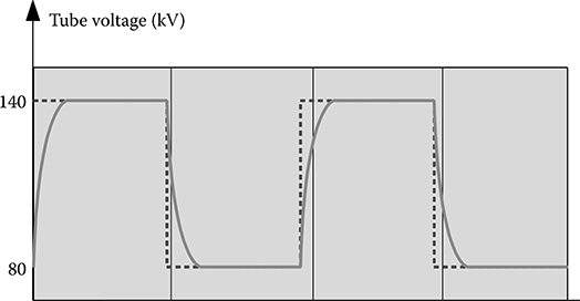
FIGURE 6.3
The rise and fall of actual kVp form complicates the spectral calibration of FKS dual-energy CT.

where

S_k(E) are the basis spectra of the single kVp

N_k is the total number of the basis spectra

α_k are the weights of the basis spectra

The self-normalized detector response to this spectrum can be written as follows:

R (d) = \frac{\int_{E} \sum_{k} α_{k} S_{k} (E) E [1 - e^{- μ_{d} (E) t_{d}}] e^{\sum_{b} μ_{b} (E, d) I_{b} (d)}}{\sum_{d} \int_{k} α_{k} S_{k} (E) E [1 - e^{- μ_{d} (E) t_{d}}] e^{- \sum_{b} μ_{b} (E, d) I_{b} (d)} d E}, (6.2)

$R (d) = \frac{\int_{E} \sum_{k} α_{k} S_{k} (E) E [1 - e^{- μ_{d} (E) t_{d}}] e^{\sum_{b} μ_{b} (E, d) I_{b} (d)}}{\sum_{d} \int_{k} α_{k} S_{k} (E) E [1 - e^{- μ_{d} (E) t_{d}}] e^{- \sum_{b} μ_{b} (E, d) I_{b} (d)} d E}, (6.2)$

in which μ_d(E) is the linear attenuation coefficient of the detectors, t_d is detector thickness, and μ_b(E,d) and I_b(d) are, respectively, the linear attenuation coefficient and the thickness of bow tie material b corresponding to detector channel d. If we denote

G_{k} (d) = \int_{E} S_{k} (E) E [1 - e^{- μ_{d} (E) t_{d}}] e^{- \sum_{b} μ_{b} (E, d) I_{b} (d)} d E, (6.3)

$G_{k} (d) = \int_{E} S_{k} (E) E [1 - e^{- μ_{d} (E) t_{d}}] e^{- \sum_{b} μ_{b} (E, d) I_{b} (d)} d E, (6.3)$

Equation 6.2 can be simplified to

R (d) = \frac{\sum_{k} α_{k} G_{k} (d)}{\sum_{d} \sum_{k} α_{k} G_{k} (d)} . (6.4)

$R (d) = \frac{\sum_{k} α_{k} G_{k} (d)}{\sum_{d} \sum_{k} α_{k} G_{k} (d)} . (6.4)$

R(d) can be measured through a fast switching air scan, and G_k(d) can be calculated based on the system geometry. Hereby the weighting coefficients α_k can be solved from Equation 6.4 by least-square fitting. The overall spectrum is decomposed into a superposition of several basis spectra through the measurement of the detector response to the bow tie attenuation.

The earlier mentioned spectrum estimation technique is graphically demonstrated in Figure 6.4. P_c(I) represents the equivalent x-ray attenuation of the estimated spectrum by Equation 6.4. P(V_e,I) is the measured x-ray attenuation of the fast-kVp system. It is obvious that the estimated spectrum P_c(I) matches the actual spectrum P(V_e,I) with minimal difference.

6.1.2.2 Detector

The detector is a key contributor to FKS acquisitions through its scintillator and data acquisition system. Detector primary decay and afterglow performance are critical to avoiding spectral blurring between views. Primary speed and afterglow refer to the decays of light emitting from the scintillator for several to tens of milliseconds after the x-ray source is switched off. This phenomenon is analogous to the decay of light signal on the television screen after it is turned off. The residual signal from one view smears information contained in the next during a scan, thereby causing degradation of spatial resolution and undesirable cross-contamination of spectra.

Images

FIGURE 6.4
The estimation of effective spectrum in FKS dual-energy CT imaging. P_c(I) represents the equivalent x-ray attenuation of the estimated spectrum by Equation 6.4. P(V_e,I) is the measured x-ray attenuation of the fast-kVp system. It is obvious that the estimated spectrum P_c(I) matches the actual spectrum P(V_e,I) with minimal difference. (Image courtesy of Dr Dan Xu of GE Global Research, Schenectady, NY.)

Gemstone scintillator material (GE Healthcare, Waukesha, WI) is a complex rare earth-based oxide, which has a chemically replicated garnet crystal structure. This lends itself to imaging that requires high light output, fast primary speed, and very low afterglow. Gemstone has a primary speed of only 30 ns, or 100 times faster than GOS (Gd₂O₂S), while also having afterglow that is only 20% of GOS, making it ideal for fast sampling [20]. For illustration we depict in Figure 6.5 a decay curve of a Gemstone detector. The capabilities of the scintillator are also paired with an ultrafast data acquisition system (up to 7 kHz), enabling simultaneous acquisition of low- and high-kVp data at customary rotation speeds.

6.1.2.3 Flux

Compared to SE CT, the traditional flux issues are more challenging in FKS dual-energy CT imaging. There hereby needs to be a strategy for balancing the flux between the two spectra and a need for noise reduction processing (which will be discussed later in Section 6.1.4).

Images

FIGURE 6.5
Gemstone scintillator material (GE Healthcare, Waukesha, WI) has a primary speed of only 30 ns, or 100 times faster than GOS (Gd₂O₂S), while also having afterglow that is only 20% of GOS, making it ideal for fast sampling. (Image courtesy of Dr Haochuan Jiang, GE Healthcare, Waukesha, WI.)

Figure 6.6 illustrates a simplified FKS dual-energy abdominal CT exam acquisition timing sequence in comparison with that of a SE abdominal CT vexam. The number of views in FKS dual-energy acquisition doubles those for SE, while the x-ray exposure time remains either the same (in abdomen cases) or similar (in head cases) as the SE acquisition. This results in much shorter view time for FKS dual-energy acquisition. As illustrated, the exposure time of a 140 kVp view in FKS dual-energy acquisition is roughly 40% of that of a single-energy view.

In dual-energy imaging, the flux ratio between the low and high kVps is in general constrained in such way that the contrast-to-noise ratio (CNR) is maximized. Multiple studies [21–23] have suggested the CNR is maxi-mized with ∼30% flux allocation, defined as the percentage of entrance skin exposure of the low kVp to that of the low and high kVp combined. That is, roughly speaking, the exposure ratio between the low and high kVps is

\frac{N_{L}}{N_{H}} = \frac{1}{2} . (6.5)

$\frac{N_{L}}{N_{H}} = \frac{1}{2} . (6.5)$

The x-ray exposure is a function of x-ray energy spectrum, beam filtration, geometry, and the tube current–time product (mAs). The FKS dual-energy CT system employs identical geometry and beam filtration for the 140 and 80 kVp acquisitions, which leaves only mAs adjustable. For the x-ray tubes used in CT, the x-ray exposure of a 140 kVp beam is roughly threefold of that of an 80 kVp beam [24]. Therefore, according to Equation 6.5, the mAs ratio between low- and high-kVp views should be kept around 3/2.

Images

FIGURE 6.6
Comparison of the simplified acquisition timing sequence between a FKS dual-energy abdominal CT exam and a SE abdominal CT exam. The number of views in FKS dual-energy acquisition doubles those for SE, while the x-ray exposure time remains either the same (in abdomen cases) or similar (in head cases) as the SE acquisition. This results in much shorter view time for FKS dual-energy acquisition. As illustrated, the exposure time of a 140 kVp view in FKS dual-energy acquisition is roughly 40% of that of a sing-energy view. (Adapted from Li, G. et al., Med. Phys., 38(5), 2595, 2011.)

In theory, there are two potential approaches to achieve the desired flux ratio: one, modulating the tube current while maintaining constant view time (i.e., exposure time in milliseconds per view) and, two, modulating the view time while maintaining constant tube current.

Modulating the tube current is conceptually more straightforward; however, it faces an implementation dilemma. Since higher tube current is required for 80 kVp view, the filament is at a very high temperature. Upon switching to 140 kVp, which mandates a much lower tube current, it requires a mechanism to reverse the polarization between the anode and cathode, at several kilohertz, to “pinch” the flow of electrons in order to lower the current.

Hence, modulating the view time while maintaining constant tube current is the preferred approach in FKS dual-energy CT imaging for flux control [13,14]. Based on the earlier mentioned analysis, the view time ratio between the low- and high-kVp views should be 60%–40%. To demonstrate the importance of balancing flux through modulating the view time in FKS dual-energy CT imaging, we simulate a low-contrast lesion (2 cm in diameter) embedded in an oval phantom. Figure 6.7 summarizes the results from the simulation and shows the impact of various view time ratios on the image quality. Comparing the results, 60%–40% view time ratio clearly offers the best CNR for the lesion detection.

Images

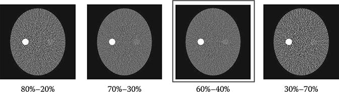
FIGURE 6.7
The reconstructed images of a simulated low-contrast lesion (2 cm in diameter) embedded in an oval phantom. The simulations were conducted under identical conditions except for the view time ratio. The view time ratio is defined as the percentage of low-kVp view to high-kVp view in each low–high-kVp pair. Comparing the results, 60%–40% view time ratio clearly offers the best CNR for the lesion detection. The result demonstrates the importance of balancing flux through modulating the view time in FKS dual-energy CT imaging.

6.1.2.4 Dose

FKS dual-energy CT has been designed to minimize the additional dose relative to SE. In a recent dose and low-contrast detectability (LCD) comparison [13,14], the effectiveness of this sampling scheme with respect to dose was demonstrated by matching the LCD at a slice thickness equal to 5 mm and object size of 3 mm.

In x-ray CT imaging, dose, resolution, and noise are interdependent quantities. Thereby, it is less useful to compare dose between two systems without first equalizing the other two parameters. If the FKS dual-energy CT employs identical geometry and beam filtration as the SE CT, previous study has shown no significant difference in measured spatial resolution between the two systems, when the reconstruction kernel and display field of view are matched [25].

Therefore, for a fair comparison of dose, one only needs to equalize the amount of image noise. The LCD is a clinical-relevant image quality metric that quantifies image noise performance, making it ideal as an image quality target when measuring dose. The lower the LCD is, the less contrast a lesion of certain size (in mm) must have in order to be detected at a given confi-dence level (usually 95%).

Traditionally, the LCD is measured by visually detecting low-contrast objects on a specially designed phantom. An example of a popular phantom (Catphan 600, Phantom Laboratory, Salem, NY) is displayed in Figure 6.8a. The disadvantage of this approach is, not surprisingly, that the results are subjective to many conditions, including inter-reader variability, viewing conditions, and whether or not artifacts are present.

Images

FIGURE 6.8
(a) An example of visual LCD phantom. The results are subjective to many conditions, including inter-reader variability, viewing conditions, and presence of artifacts. (b) A square array of ROIs placed in the uniform water-equivalent section of the Catphan 600 phantom. Each ROI is 6 pixels by 6 pixels that has an equivalent area to a circular object of 3 mm in diameter (DFOV = 22.7 cm, 512 × 512 image matrix). (c) By measuring the distribution of mean CT#’s of many ROIs, a prediction can be made for the necessary CT# of a low-contrast object the same size as the ROIs in order to detect it at a 95% confidence level. (Adapted from Li, G. et. al., Med. Phys., 38(5), 2595, 2011.)

An automated statistical LCD method is thus more desirable. Chao et al. has developed one of such tools [26]. The processing begins with placing a square array of region of interest (ROI) on a uniform water-equivalent section of the Catphan 600, as depicted in Figure 6.8b. Each ROI is 6 pixels by 6 pixels, which has an area equivalent to a circular object of 3 mm in diameter for a 22.7 cm DFOV and 512 × 512 matrix sizes. As shown in Figure 6.8c, the distribution of mean CT number of the ROIs provides an estimate of the necessary contrast (in CT number) in order to detect a low-contrast object the same size as the ROIs at a 95% confidence level.

Figure 6.9 compares the measured CTDI_vol (in mGy) between a FKS dual-energy and routine (i.e., SE) abdominal CT exams as a function of monochromatic energy (in keV, dual-energy only) and tube current (in mA, SE only). The SE measurements are denoted as “SE xxx mA,” where “xxx” describes the tube current, while the dual-energy measurements are denoted as “Mono xx keV,” where “xx” represents the monochromatic energy (monochromatic energy will be discussed later in Section 6.1.3.2). All other acquisition protocols were the same between the two systems compared (kVp = 120 kVp, gantry rotate speed = 1.0 s, bow tie = large body, slice thickness = 5 mm, display field of view = 22.5 cm).

From Figure 6.9, one can see that, with a tube current of 360 mA, the SE abdominal CT exam yields a LCD of 0.426% and a CTDI_vol of 29.2 mGy for a 3 mm object. The FKS dual-energy abdominal CT exam (65 keV) produces a nearly identical LCD of 0.422% (0.01% = 0.1 HU) with a CTDI_vol of 33.43 mGy for the same object size, or just 14% higher than that of a routine SE abdominal CT exam. These results were obtained using the uniform section of Catphan 600 phantom, which represents a patient with ∼20 cm water-equivalent diameter.

Images

FIGURE 6.9
Comparison of the measured CTDI_vol (in mGy) between a FKS dual-energy and routine (i.e., SE) abdominal CT exams as a function of monochromatic energy (in keV, dual-energy only) and tube current (in mA, SE only) (all other acquisition protocols were the same between the two systems compared: kVp = 120 kVp, gantry rotate speed = 1.0 s, bow tie = large body, slice thickness = 5 mm, display field of view = 22.5 cm). The SE measurements are denoted as “SE xxx mA,” where “xxx” describes the tube current, while the dual-energy measurements are denoted as “Mono xx keV,” where “xx” represents the monochromatic energy (monochromatic energy will be discussed later in Section 6.1.3.3). All other acquisition protocols (kVp, gantry rotation speed, bow tie, slice thickness, display field of view, etc.) were the same between the two systems compared. (Adapted from Li, G. et. al., Med. Phys., 38(5), 2595, 2011.)

6.1.3 Image Reconstruction

6.1.3.1 Projection-Space Material Decomposition

The mass attenuation coefficient across the x-ray spectrum is a function of two independent variables: photoelectric effect and Compton scatter [1]. Based on this principle, the low- and high-kVp projection data can be retrospectively transformed into a pair of basis materials (such as water and iodine).

Through a mathematical change of basis, one can express the energy-dependent attenuation observed in two kVp measurements in terms of two basis materials [14]:

\begin{matrix} f_{1} (\vec{l}) = α_{1} p_{H} (\vec{l}) + β_{1} p_{L} (\vec{l}) + χ_{1} p_{H}^{2} (\vec{l}) + δ_{1} p_{L}^{2} (\vec{l}) + ε_{1} p_{H} (\vec{l}) p_{L} (\vec{l}) + \dots \\ f_{2} (\vec{l})= α_{2} p_{H} (\vec{l})+ β_{2} p_{L} (\vec{l})+ χ_{2} p_{H}^{2} (\vec{l})+ δ_{2} p_{L}^{2} (\vec{l})+ ε_{2} p_{H} (\vec{l}) p_{L} (\vec{l})+ \dots . \end{matrix} (6.6)

$\begin{matrix} f_{1} (\vec{l}) = α_{1} p_{H} (\vec{l}) + β_{1} p_{L} (\vec{l}) + χ_{1} p_{H}^{2} (\vec{l}) + δ_{1} p_{L}^{2} (\vec{l}) + ε_{1} p_{H} (\vec{l}) p_{L} (\vec{l}) + \dots \\ f_{2} (\vec{l})= α_{2} p_{H} (\vec{l})+ β_{2} p_{L} (\vec{l})+ χ_{2} p_{H}^{2} (\vec{l})+ δ_{2} p_{L}^{2} (\vec{l})+ ε_{2} p_{H} (\vec{l}) p_{L} (\vec{l})+ \dots . \end{matrix} (6.6)$

where

$\vec{l}$ $\vec{l}$ is an arbitrary ray path,

$P_{H} (\vec{l})$ $P_{H} (\vec{l})$ and $P_{L} (\vec{l})$ $P_{L} (\vec{l})$ denote the high- and low-kVp projection data,

$f_{i} (\vec{l})$ $f_{i} (\vec{l})$ represents the density of the basis material i,

α, β, ξ, δ, ∊ that are polynomial coefficients,

H and L refer to the high and low kVps, respectively.

There are a couple of important facts in Equation 6.6 that should be noted here. First of all, $P_{H} (\vec{l})$ $P_{H} (\vec{l})$ and $P_{L} (\vec{l})$ $P_{L} (\vec{l})$ must be measured along the same ray path $\vec{l}$ $\vec{l}$ . This can be easily satisfied by FKS dual-energy CT imaging. The FKS mechanism ensures the low- and high-kVp projection data are spatially and temporally co-registered. (Note: Strictly speaking, the low- and high-kVp views incur a small angular offset relative to each other. To obtain truly co-registered projection pair, these views are interpolated to the same angular positions prior to material decomposition.)

Secondly, the high-order terms in Equation 6.6 are critically important to account for spectral variation over the field of view due to source spectrum, bow tie filter, detector performance, and multi-material beam-hardening effects [1]. As a consequence, projection-space material decomposition provides the opportunity for more quantitative precision than what may be achieved with SE imaging. This is the key difference between FKS dual-energy CT imaging and image-space dual-energy CT imaging, which usually require a post-reconstruction beam-hardening correction to recover, hopefully, the spectral information that has been lost during the image reconstruction.

Images

FIGURE 6.10
Equation 6.6 is overdetermined and the resolution for polynomial coefficients α, β, ξ, δ, ∊, etc. can be found easily through least-square fitting defined by Equation 6.7. The vertical axis represents the thickness of water.

To solve Equation 6.6, dual-energy projection data corresponding to different thicknesses of water and iodine are acquired. Since modern CT scanners contain a large number of detector elements, Equation 6.6 is overdetermined and the resolution for polynomial coefficients α, β, ξ, δ, ∊, etc. can be found easily through least-square fitting:

\begin{array}{l} \arg \min \underset{\vec{l}}{\sum^{​}} ‖ f_{1} (\vec{l})- α_{1} p_{H} (\vec{l})- β_{1} p_{L} (\vec{l})- χ_{1} p_{H}^{2} (\vec{l})- δ_{1} p_{L}^{2} (\vec{l})- ε_{1} p_{H} (\vec{l}) p_{L} (\vec{l})- … ‖^{2} \\ \arg \min \underset{\vec{l}}{\sum^{​}} ‖ f_{2} (\vec{l})- α_{2} p_{H} (\vec{l})- β_{2} p_{L} (\vec{l})- χ_{2} p_{H}^{2} (\vec{l})- δ_{2} p_{L}^{2} (\vec{l})- ε_{2} p_{H} (\vec{l}) p_{L} (\vec{l})- … ‖^{2} . \end{array} (6.7)

$\begin{array}{l} \arg \min \underset{\vec{l}}{\sum^{}} ‖ f_{1} (\vec{l})- α_{1} p_{H} (\vec{l})- β_{1} p_{L} (\vec{l})- χ_{1} p_{H}^{2} (\vec{l})- δ_{1} p_{L}^{2} (\vec{l})- ε_{1} p_{H} (\vec{l}) p_{L} (\vec{l})- … ‖^{2} \\ \arg \min \underset{\vec{l}}{\sum^{}} ‖ f_{2} (\vec{l})- α_{2} p_{H} (\vec{l})- β_{2} p_{L} (\vec{l})- χ_{2} p_{H}^{2} (\vec{l})- δ_{2} p_{L}^{2} (\vec{l})- ε_{2} p_{H} (\vec{l}) p_{L} (\vec{l})- … ‖^{2} . \end{array} (6.7)$

Figure 6.10 shows such an example. The vertical axis represents the thickness of water.

6.1.3.2 Image Reconstruction

Through material decomposition, the energy-dependent attenuation measurements contained in kVp projections are transformed into energy-independent basis material projection data corresponding to the two basis material pair (e.g., water and iodine). Although the pair of basis material projection data (sinogram) essentially contains all useful information about the material being imaged, they are difficult to understand and interpreted by clinicians. A more useful form, which clinicians are familiar with, is the reconstructed images.

Having the identical geometry, the same reconstruction algorithm to reconstruct the SE CT images can therefore be applied to the first basis material projection data to obtain the corresponding basis material density image. The step is repeated for the second basis material as well. An example is shown in Figure 6.11. Basis material density images represent the effective density for the anatomies necessary to create the observed low- and high-kVp attenuation measurements. For instance, pure water appears as 1000 mg/cc in a water density image, and 50 mg/cc of diluted iodine is labeled as such in an iodine density image, etc. Any non-basis material is mapped to both basis materials. For this reason, basis material density images are sometimes called “material density map.”

Images

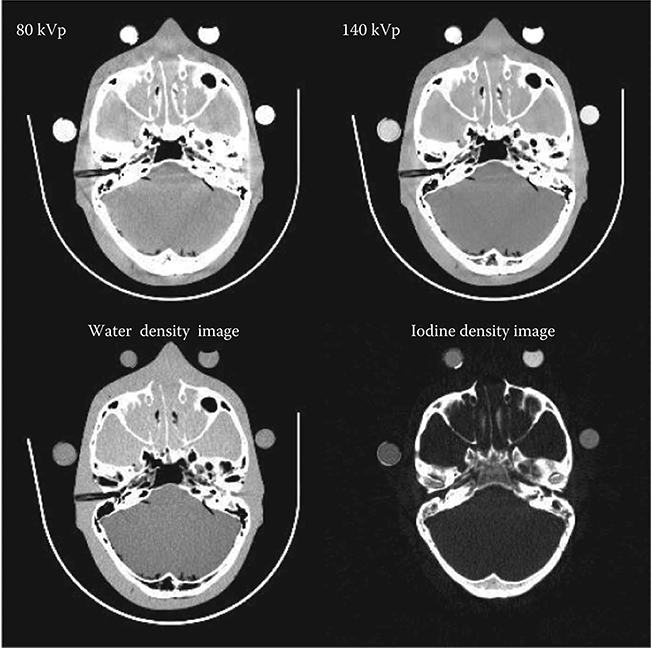
FIGURE 6.11
Exemplary reconstructed basis material density images, as well as the kVp images, from a FKS dual-energy head CT exam.

6.1.3.3 Monochromatic Energy Image

Given the material basis density images, one can compute attenuation data that would be measured with a monoenergetic x-ray source by combining the material density images to create a monochromatic image at any specific energy level (in keV), E [14]:

\int^{​} u (\vec{l}, E) d l =(\frac{μ_{1}}{p_{1}})(E) \int^{​} f_{1} (\vec{l}) d l +(\frac{μ_{2}}{p_{2}})(E) \int^{​} f_{2} (\vec{l}) d l (6.8)

$\int^{} u (\vec{l}, E) d l =(\frac{μ_{1}}{p_{1}})(E) \int^{} f_{1} (\vec{l}) d l +(\frac{μ_{2}}{p_{2}})(E) \int^{} f_{2} (\vec{l}) d l (6.8)$

where (μ_i/ρ_i) represents the mass attenuation coefficient for material i. For consistency with the Hounsfield unit (HU), one can normalize the attenuation measurement with respect to water. A clinical example is shown in Figure 6.12.

From Equation 6.8, the expected image noise (variance) in the monochromatic image can be expressed based on linear system theory and noise propagation principle:

δ_{m o n o}^{2} = {[(\frac{μ_{1}}{p_{1}}) (E)]}^{2} σ_{f_{1}}^{2} + {[(\frac{μ_{2}}{p_{2}}) (E)]}^{2} σ_{f_{2}}^{2} . (6.9)

$δ_{m o n o}^{2} = {[(\frac{μ_{1}}{p_{1}}) (E)]}^{2} σ_{f_{1}}^{2} + {[(\frac{μ_{2}}{p_{2}}) (E)]}^{2} σ_{f_{2}}^{2} . (6.9)$

Equation 6.9 implies that the noise in the generated monochromatic energy image is also energy dependent. This has been confirmed through phantom experiment. Figure 6.13 plots the measured noise (in HU) as a function of monochromatic energy level, in the range of 40–140 keV, for a 20 cm water phantom. The noise curve exhibits a global minimum near 65 keV for the particular acquisition protocol.

Images

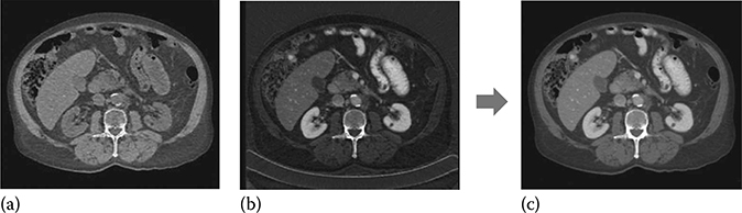
FIGURE 6.12
Reconstruction of monochromatic energy image from a pair of basis material density images. The monochromatic energy image, which represents attenuation data that would be measured with a monoenergetic x-ray source at any specific keV level, is computed by combining the basis material density images using Equation 6.8. (a) Water density (mg/cc), (b) iodine density (mg/cc), and (c) 65 keV monochromatic (HU).

Images

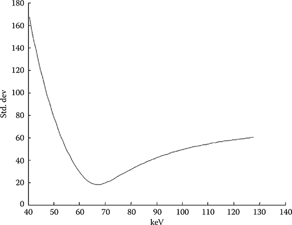
FIGURE 6.13
The noise in the generated monochromatic energy images is energy dependent. For FKS dual-energy CT imaging, the noise curve exhibits a global minimum near 65 keV for the particular acquisition protocol. (Adapted from Li, G. et. al., Med. Phys., 38(5), 2595, 2011.)

6.1.3.4 Effective Atomic Number

The x-ray linear attenuation coefficient of a periodic element, μ, can be expressed as a function of the element's material properties and E:

(\frac{μ}{ρ}) (E) = σ (E) \frac{N_{A}}{A}, (6.10)

$(\frac{μ}{ρ}) (E) = σ (E) \frac{N_{A}}{A}, (6.10)$

where σ, N_A, and A are the total effective cross section, Avogadro's number, and the mass number.

The total effective cross section of x-ray radiation in function of the chemical composition of the materials can be modeled as a combination of the Compton and photoelectric effects [27]:

σ (E) = a (E) Z_{e f f} + b (E) Z_{e f f}^{C (E)}, (6.11)

$σ (E) = a (E) Z_{e f f} + b (E) Z_{e f f}^{C (E)}, (6.11)$

where Z_eff is the effective atomic number. The coefficients a, b, and c depend only on the energy and their values can be obtained from NIST [28].

By substituting (6.11) into (6.10), the linear attenuation can be further expressed as

μ (E) = (a (E) Z_{e f f} + b (E) Z_{e f f}^{C (E)}) \frac{N_{A} ρ}{A} . (6.12)

$μ (E) = (a (E) Z_{e f f} + b (E) Z_{e f f}^{C (E)}) \frac{N_{A} ρ}{A} . (6.12)$

The simultaneous equations are formed using Equation 6.12 for two monochromatic energy images μ(E₁) and μ(E₂). Solving the simultaneous equations, Z and ρ can be obtained as follows:

Z_{e f f} = {[\frac{A}{N_{A} ρ} \cdot \frac{a (E_{2}) μ (E_{1}) - a (E_{1}) μ (E_{2})}{a (E_{2}) b (E_{1}) - a (E_{1}) b (E_{2})}]}^{1 / C (E)} . (6.13)

$Z_{e f f} = {[\frac{A}{N_{A} ρ} \cdot \frac{a (E_{2}) μ (E_{1}) - a (E_{1}) μ (E_{2})}{a (E_{2}) b (E_{1}) - a (E_{1}) b (E_{2})}]}^{1 / C (E)} . (6.13)$

Z_eff describes the periodic elements most closely representing its energy-dependent attenuation behavior; hence it often provides insight regarding the material's chemical composition. Knowledge of the effective atomic number of critical tissue types or specific contrast agents may be leveraged to define and import custom basis materials, allowing for the enhancement of specific anatomical structures.

Figure 6.14 shows graphically the distribution of several materials commonly encountered in diagnostic radiology in the basis material space (water and bone). Materials are clearly separated based on their chemical decomposition. The effective atomic number of each material is reflected by the angular slope. Noise is primarily responsible for the scatter of points in each material and the overlap between different materials.

6.1.4 Noise Suppression

It is well known that the basis material density images have a much lower signal-to-noise ratio (SNR) than SE CT images. This can be easily demonstrated by the following simple analysis. Let's define the SNR of iodine in a low-kVp image as

{SNR}_{L} (x, y) \propto \frac{μ_{L}^{l} (x, y)}{σ_{L} (x, y)} . (6.14)

${SNR}_{L} (x, y) \propto \frac{μ_{L}^{l} (x, y)}{σ_{L} (x, y)} . (6.14)$

Then the SNR of iodine in a basis material density image is

{SNR}_{Δ E} (x, y) \propto \frac{μ_{L}^{l} (x, y) - R^{T} μ_{H}^{l} (x, y)}{\sqrt{σ_{L}^{2} (x, y) + {(R^{T})}^{2} σ_{H}^{2} (x, y)}} . (6.15)

${SNR}_{Δ E} (x, y) \propto \frac{μ_{L}^{l} (x, y) - R^{T} μ_{H}^{l} (x, y)}{\sqrt{σ_{L}^{2} (x, y) + {(R^{T})}^{2} σ_{H}^{2} (x, y)}} . (6.15)$

Images

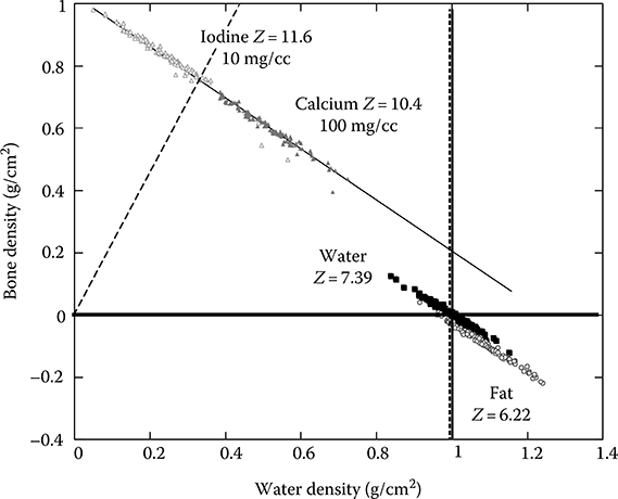
FIGURE 6.14
Graphic representation of several materials commonly encountered in diagnostic radiology in the plane of two basis materials (water and bone). Materials are clearly separated based on their chemical decomposition. The effective atomic number of each material is reflected by the angular slope. Noise is primarily responsible for the scatter of points in each material and the overlap between different materials.

By comparing (6.2) with (6.1) and using the fact that $μ_{L}^{I}$ $μ_{L}^{I}$ and $μ_{H}^{I}$ $μ_{H}^{I}$ are very close for the most of relevant energy levels, we can conclude that

{SNR}_{Δ E} (x, y) ≪ {SNR}_{L} . (6.16)

${SNR}_{Δ E} (x, y) ≪ {SNR}_{L} . (6.16)$

A reduction of noise can be achieved by increased exposure. But based on x-ray physics, a noise reduction by a factor of n requires an exposure increase by a factor of n², which leads to unacceptable dose levels for most patients. Therefore, noise suppression has to be automatically applied to FKS dual-energy CT imaging and on the basis material density images in order to enhance the quality of the image while preserving the density values. This allows for a quantitative basis material density image with good image quality.

Noise reduction techniques that attempt to directly reduce noise in basis material density images have also been sought after. To this date, none of them have had success in reducing noise to satisfactory levels while minimally affecting iodine contrast without introducing artifacts.

A more significant improvement in SNR, however, results from the understanding the physical property of the noises that exist in basis material density images. It has been proven that the noises in the two resulting basis material density images are negatively correlated [2,8]. In other words,

COV (σ_{m_{1}}, σ_{m_{2}}) < 0, (6.17)

$COV (σ_{m_{1}}, σ_{m_{2}}) < 0, (6.17)$

where denote m₁ and m₂ stand for the two basis material images.

Taking advantage of the property in Equation 6.17, several noise suppression algorithms have been developed [8,29]. These algorithms subtract a weighted high-pass filtered version of the first basis material density image (e.g., water) to noise reduce the complimentary basis material density image (e.g., iodine).

These algorithms are effective in suppressing noise. However, they are at the risk of introducing a detrimental artifact. Although the high-pass filtered image is smoothed, edge structures and blood vessels full of contrast medium are added to the complimentary basis material density image, causing “cross-contamination” that changes the accuracy of the density values.

The solution, however, exists if a two-pass algorithm is employed. Upon the completion of the first pass, the noise masks from both basis material density images are generated and combined at certain energy to create a monochromatic energy image of the noises. As shown in Figure 6.15a, this image contains a large amount of edge structures and iodinated blood vessels as a result of cross-contamination. One can project these structures back to the basis material density images, where a high-pass filter is applied adaptively to both basis material density images. This second pass filter results in updated noise masks that have significantly less contamination-prune structures (Figure 6.15b and c). Reduction of contamination-prune structures is evident. The updated noise masks are then added to the complimentary basis material density image for noise suppression.

The effectiveness of the proposed two-pass algorithm is demonstrated in Figure 6.16. In this clinical example, the original water and iodine density images are very noisy. Noise-reduced water density image using a single-pass algorithm, where the cross-contaminated structures are clearly visible throughout the liver area. By comparing the complimentary noise-reduced iodine density image, one can correlate the contaminations in the water density image with the iodinated hepatic vessels in iodine density images. Using the two-pass algorithm, noise-reduced water density image is free of contamination.

6.1.5 Visualization and Clinical Applications

FKS dual-energy CT imaging provides diagnostic information beyond that found in conventional SE CT imaging, in a manner consistent with workflow, and that increases the efficacy of clinical diagnosis. The clinical application and visualization of dual-energy data is presently an area of active research.

FKS dual-energy CT images can be reviewed and quantified in a number of ways. Most commonly, it is visualized as a monochromatic energy image, which resembles a conventional kVp image, but with fewer beam-hardening artifacts. One may interactively change the energy level from 40 to 140 keV to best balance the needs in terms of contrast and noise. It is also common to visualize the data as a basis material density image pair. Specific material density can be directly measured from these images, which form the basis for differentiation of certain tissue of clinical interest. For example, based on the relative density of a hepatic cyst with respect to water, one can determine if the cyst is water or fat based, which may be important for making a proper diagnosis. In an effort to simplify the workflow and minimize the workload, the iodine density image can be displayed as a color overlay on the monochromatic image.

Images

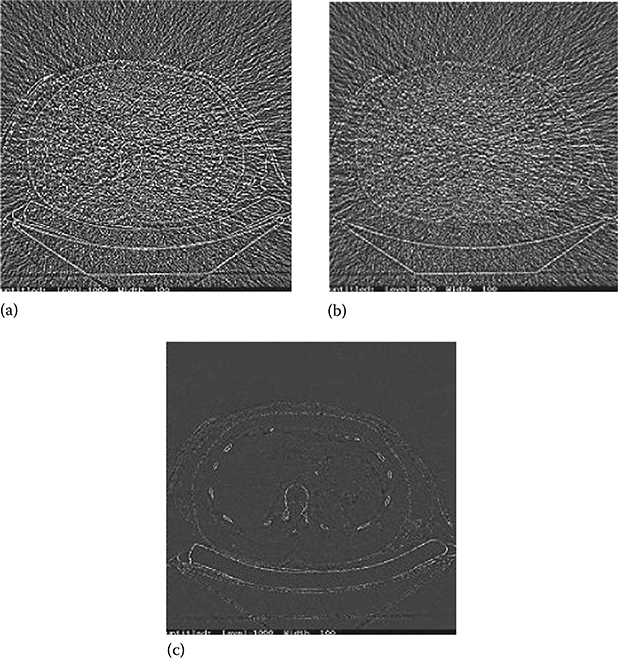
FIGURE 6.15
Example of noise mask generated from a water density image. (a) Uncorrected noise mask. Structures such as vertebrae and ribs can be clearly seen. (b) Corrected noise mask after applying the proposed algorithm. (c) The difference image between (a) and (b). Removing of the structures is evident.

One can also visualize dual-energy data as the effective atomic number, Z_eff, of the materials. This information provides insight into the material's chemical composition. Alternatively, different materials can be described as histograms or scatterplots, as the example shown earlier in Figure 6.14.

To further identify trends and support additional knowledge from the data, the attenuation profile of the material versus keV may also be graphically depicted by a tissue signature curve. An example is demonstrated in Figure 6.17.

Research into FKS dual-energy CT imaging has been conducted in multiple clinical applications. A discussion of abdominal applications may be found in [15,30]. More recently, attention has been given to apply FKS dual-energy CT imaging to cardiac applications, due to its excellent temporal–spatial resolution and potential for reduced beam hardening in myocardium and reduced calcium blooming. In one study, reduced calcium blooming has increased accuracy in coronary stenosis sizing through improved differentiation of calcified plaque and iodinated contrast lumen, enabling accurate measurement and risk profiles of lipid (cholesterol) plaques [18].

Images

FIGURE 6.16
Example of noise suppression of a FKS dual-energy CT imaging using the two-pass algorithm. (a) Original water density image. (b) Original iodine density image. (c) Noise-reduced water density image using a single-pass algorithm, where the cross-contaminated structures are clearly visible throughout the liver area. (d) Noise-reduced iodine density image using a single-pass algorithm. The iodinated hepatic vessels are the root cause of the cross-contaminations seen in the complimentary water image in (c). (e) Noise-reduced water density image using the two-pass algorithm is free of contamination. (f) Noise-reduced iodine density image using the two-pass algorithm.

Images

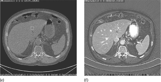
FIGURE 6.17
Tissue signature curves of two pulmonary masses, which are highlighted in the monochromatic energy image, demonstrate different behaviors in this FDK dual-energy exam. Biopsy procedures have confirmed mass 1 (upper left on image, topmost curve on graph) is a malignant nodule and mass 2 (lower right mass on image, lowest curve on graph) a calcified nodule (benign). (Image courtesy of Dr Amy Hara, Mayo Clinic, Scottsdale, AZ.)

Thanks to its inherent beam-hardening reduction capability, FKS dual-energy CT imaging has increased accuracy in hip implant assessment through improved differentiation of hip bone and metallic implant, enabling accurate measurement of joint spacing (Figure 6.18).

Images

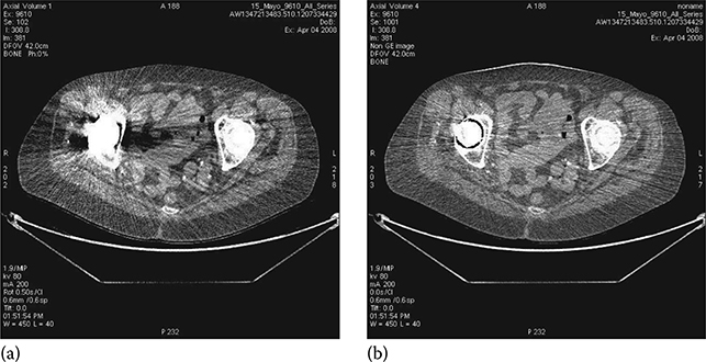
FIGURE 6.18
Example of metal artifact reduction of FKS dual-energy CT imaging. (a) SE CT exam. (b) FKS dual-energy CT exam. (Image courtesy of Robert Beckett, GE Healthcare, Waukesha, WI.)

Another excellent example of metal artifacts from pedicle screws is shown in sagittal reformatted postoperative spinal CT (Figure 6.19a). The reconstructed FKS dual-energy CT image displays significantly less streak artifacts, enabling much improved visualization of the dural sac and spinal muscles.

Images

FIGURE 6.19
Example of metal artifact reduction of FKS dual-energy CT imaging. (a) SE CT exam. (b) FKS dual-energy CT exam. (Image courtesy of Dr. Amy Hara, Mayo Clinic, Scottsdale, AZ.)

References

1. R. Alvarez and A. Macovski, Energy-selective reconstructions in x-ray CT, Phys. Med. Biol. 21(5), 733–744, 1976.

2. R. Alvarez and E. Seppi, A comparison of noise and dose in conventional and energy selective computed tomography, IEEE Trans. Nucl. Sci. 26(2), 2853–2856, 1979.

3. H. Genant and D. Boyd, Quantitative bone mineral analysis using dual energy computed tomography, Invest. Radiol. 12, 545–551, 1977.

4. C. Cann, G. Gamsu, F. Birnberg, and W. Webb, Quantification of calcium in solitary pulmonary nodules using single- and dual-energy CT, Radiology 145, 493–496, 1982.

5. A. Coleman and M. Sinclair, A beam-hardening correction using dual-energy computed tomography, Phys. Med. Biol. 30(11), 1251–1256, 1985.

6. W. Kalender, W. Perman, J. Vetter, and E. Klotz, Evaluation of a prototype dual-energy computed tomographic apparatus. I. Phantom studies, Med. Phys. 13(3), 334–339, 1986.

7. J. Vetter, W. Perman, W. Kalender, R. Mazess, and J. Holden, Evaluation of a prototype dual-energy computed tomographic apparatus. II. Determination of vertebral bone mineral content, Med. Phys. 13(3), 340–343, 1986.

8. W. Kalender, E. Klotz, and L. Kostaridou, An algorithm for noise suppression in dual energy CT material density images, IEEE Trans. Med. Imag. 7(3), 218–224, 1988.

9. S. Sengupta, S. Jha, D. Walter, Y. Du, and E. Tkaczyk, Dual energy for material differentiation in coronary arteries using electron-beam CT, Proc. SPIE Med. Imag. 5745, 1306–1316, 2005.

10. C. Maaβ, M. Baer, and M. Kachelrieβ, Image-based dual energy CT using opti-mized precorrection functions: A practical new approach of material decomposition in image domain, Med. Phys. 36(8), 3818–3829, 2009.

11. A. Altman and R. Carmi, A double-layer detector dual-energy CT—Principles, advantages and applications, Med. Phys. 36(6), 2750, 2009.

12. J. Hsieh, Dual-energy CT with fast-kVp switching, Med. Phys. 36(6), 2749, 2009.

13. B. Li, G. Yadava, and J. Hsieh, Head and body CTDIw of dual energy x-ray CT with fast-kVp switching, Proc. SPIE Med. Imag. 7622, 76221Y, 2010.

14. B. Li, G. Yadava, and J. Hsieh, Head and body CTDIw of dual energy x-ray CT with fast-kVp switching, Med. Phys. 38(5), 2595–2601, 2011.

15. A. Silva, A. Hara, R. Paden, W. Pavlicek, and B. Morse, Dual energy (spectral) CT for routine clinical abdominal imaging, Radiographics 31, 1031–1046, 2011.

16. A. Kemmling, I. Noelte, J. Scharf, and C. Groden, Diagnostic advantage of dual-energy CT bone removal in cerebral CT angiography for postsurgical evaluation of standard extracranial-intracranial arterial bypass, RSNA Scientific Assembly and Annual Program 2009, SSE16-02, 2009.

17. S. Miura, Y. Nishimoto, S. Kitano, J. Takahama, N. Marugami, and A. Hashimoto, Lung perfused blood volume image using dual-energy CT in patients with acute and chronic pulmonary embolism, RSNA Scientific Assembly and Annual Program 2009, LL-CH4297-B11, 2009.

18. W. Pavlicek, P. Panse, K. A. Hara, T. Boltz, R. Paden, P. Licato, N. Chandra, D. Okerlund, R. Bhotika, and D. Langan, Initial use of fast switched dual energy CT for coronary artery disease, Proc. SPIE Med. Imag. 7622, 76221V, 2010.

19. D. Xu, D. Langan, X. Wu, J. Pack, T. Benson, J. Tkaczky, and A. Schmitz, Dual energy CT via fast kVp switching spectrum estimation, Proc. SPIE Med. Imag. 7258, 72583T, 2009.

20. H. Jiang, GE healthcare's gemstone scintillator development, Proc. Mater. Sci. Tech. 3, 1796–2002, 2010.

21. S. Richard and J. Siewerdsen, Optimization of dual-energy imaging system using generalized NEQ and imaging task, Med. Phys. 34(1), 127–139, 2007.

22. N. Shkumat, J. Siewerdsen, A. Dhanantwari, D. Williams, S. Richard, N. Paul, J. Yorkston, and R. Van Metter, Optimization of image acquisition techniques for dual-energy imaging of the chest, Med. Phys. 34(10), 3904–3915, 2007.

23. J. Sabol, G. Avinash, F. Nicolas, B. Claus, and J. Zhao, The development and characterization of a dual-energy subtraction imaging system for chest radiography based on CsI:Tl amorphous silicon flat-panel technology, Proc. SPIE Med. Imag. 4320, 399–408, 2001.

24. J. Bushberg, J. Seibert, E. LeidholdtJr., and J. Boone, The Essential Physics of Medical Imaging, 2nd edn., Lippincott Williams & Wilkins, Baltimore, MD, 2002.

25. J. Fan, J. Hsieh, P. Sainath, and P. Crandal, Evaluation of the adaptive statistical iterative reconstruction technique for cardiac computed tomography imaging, Proc. SPIE Med. Imag. 8313, 83133F, 2012.

26. E. Chao, T. Toth, N. Bromberg, E. Williams, S. Fox, and D. Carleton, A statistical method of defining low contrast detectability, RSNA Scientific Assembly and Annual Program 2000, 2750–2750, 2000.

27. D. Jackson and D. Hawkes, X-ray attenuation coefficients of elements and mixture, Phys. Rep. 70, 169–233, 1981.

28. M. Berger and J. Hubbell, NIST XCOM: Photon cross section database, NIST Standard Reference Database 8 (XGAM) NBSIR 87-3597, 1998.

29. C. McCollough, M. Lysel, W. Peppler, and C. Mistretta, A correlated noise reduction algorithm for dual-energy digital subtraction angiography, Med. Phys. 16(6), 873–880, 1989.

30. M. Joshi, D. Langan, D. Sahani, A. Ramesh, S. Aluri, K. Procknow, X. Wu, R. Rahul, and D. Okerlund, Fast kV switching dual energy CT effective atomic number accuracy for kidney stone characterization, Proc. SPIE Med. Imag. 7622, 76223K, 2010.

..................Content has been hidden....................

You can't read the all page of ebook, please click here login for view all page.

Table of Contents for
6 Dual-Energy CT Imaging with Fast-kVp Switching