18 Multicoil Parallel MRI

Magnetic resonance imaging (MRI) is a safe medical imaging modality that can produce high-quality images. Other popular imaging modalities do not satisfy both these desirable properties—ultrasound is safe but generally yields images of poorer quality, whereas x-ray computer tomography (CT) can yield good-quality images but at the cost of potential health hazard. The main shortcoming of MRI (compared to ultrasound and CT) is its prolonged data acquisition time. The large scan time results in (1) inconvenience to patients as they have to spend a considerable amount of time in the scanner and (2) degradation in the quality of static MR images by introducing motion artifacts. In the past two decades, a considerable amount of effort has been expended in devising ways to reduce the scan time in MRI.

Broadly, there are two approaches to reduce the MRI scan time: hardware (i.e., physics) and software (i.e., signal processing) based approaches. In the hardware-based approach, to expedite the scan process, the internal mechanisms of the scanner are changed. The introduction of multichannel receiver coils (parallel MRI) over a single channel is a classic example of hardware-based acceleration. Software-based acceleration does not interfere with the mechanism of the scanner. The basic idea behind reducing the scan time is to acquire less samples than is conventionally required and then use a smart reconstruction technique to obtain the image.

This chapter discusses recent developments in software-based acceleration techniques for both single-channel and multichannel MRI scanners. These developments are based on the theory of compressed sensing (CS) [1–3]. CS addresses the problem of recovering a sparse signal from its undersam-pled measurements. The MRI is a classic application of CS techniques. CS has recently paved the path for accelerating MRI scans even from single-channel scanners!

Before discussing how CS has improved MRI acceleration, in Section 18.2, we will briefly discuss the theory of CS in Section 18.2. In Section 18.3, we will review recent developments in CS-based MRI acceleration for single-channel coils. Section 18.4 will discuss the application of CS in multichannel parallel MRI acquisition. Finally, in Section 18.5, the conclusions will be discussed.

18.2 Theory of Compressed Sensing

CS [1–3] studies the problem of solving an underdetermined system of linear equations whose solution is known to be a sparse vector, i.e., estimation of the vector x from the following:

y_{m \times 1} = Φ_{m \times n} x_{n \times 1} + η_{n \times 1}, m < n (18.1)

$y_{m \times 1} = Φ_{m \times n} x_{n \times 1} + η_{n \times 1}, m < n (18.1)$

where

y_m_×1 is the observation

Φ_m×n is the measurement operator

η_n×1 is the noise

In general, the inverse problem (18.3) has an infinite number of solutions. But when the solution x_n_×1 is s-sparse (s nonzeroes), the solution is typically unique [4]. Given enough processing time and computational power, one can find a solution to (18.3) by a brute force combinatorial search.

Mathematically, the combinatorial search can be represented as follows:

\min_{x} {‖ x ‖}_{0} subject to {‖ y - Φ x ‖}_{2}^{2} \leq σ (18.2)

$\min_{x} {‖ x ‖}_{0} subject to {‖ y - Φ x ‖}_{2}^{2} \leq σ (18.2)$

Here, we drop the dimensionality of the matrices and vectors to simplify the notation.

Please note that in (18.2), ‖.‖₀ is not a norm, it only counts the number of nonzeroes in the vector, and σ is proportional to the variance of the noise.

Solving the inverse problem (18.1) via (18.2) requires the number of measurements m to be only ≥ 2s. This can be understood intuitively. According to the assumption that the solution x is s-sparse, i.e., it has 2s degrees of freedom, s positions and the corresponding s values imply that it is possible to recover the image when the number of samples is more than 2s.

Unfortunately, (18.2) is an non-deterministic polynomial (NP) hard opti-mization problem; the solution x can only be recovered from 2s samples through an exhaustive search. It is possible to solve (18.2) approximately using a greedy algorithm [5–7]. To guarantee a solution, such approximate algorithms pose strict constraints on the nature of the inverse problem. In many practical situations, these constraints are not met. Fortunately, theoretical studies in CS [1–4] show that it is possible to solve the inverse problem (18.1) by allowing a convex relaxation of the NP hard objective function in (18.2) as follows:

\min_{x} {‖ x ‖}_{1} subject to {‖ y - Φ x ‖}_{2}^{2} \leq σ (18.3)

$\min_{x} {‖ x ‖}_{1} subject to {‖ y - Φ x ‖}_{2}^{2} \leq σ (18.3)$

where ‖.‖₁ is the sum of the absolute values of the vector.

The l₁-norm is the tightest convex envelope for NP hard l₀-norm. Convex optimization (18.3) guarantees a solution under far weaker constraints than required by approximate greedy algorithms. This is a strong result that guarantees the solution of an NP hard problem (18.2) by a convex relaxation that can be solved by quadratic programming (18.3). However, compared to the 2s samples required by the NP hard problem (18.2), the convex surrogate (18.3) requires considerably more samples, given by

m > C k \log (n) (18.4)

$m > C k \log (n) (18.4)$

For all practical problems, we are interested in decreasing the number of measurement samples as much as possible, but at the same time, we should also be able to recover the solution by a tractable polynomial time algorithm. Intuitively, if the value of p in the l_p-norm used in (18.5) is a fraction between zero and one, we hope to recover the solution by using less number of samples than required by (18.3). This intuition is theoretically proven in [8–11].

When the value of p lies between zero and one, the optimization problem becomes nonconvex:

\min_{x} {‖ x ‖}_{p}^{p} subject to {‖ y - Φ x ‖}_{2}^{2} \leq σ 0 < p < 1 (18.5)

$\min_{x} {‖ x ‖}_{p}^{p} subject to {‖ y - Φ x ‖}_{2}^{2} \leq σ 0 < p < 1 (18.5)$

The number of equations (samples) needed to solve the inverse problem (18.1) via nonconvex optimization (18.5) is [11]

n \geq C_{1} k + p k \log (n) (18.6)

$n \geq C_{1} k + p k \log (n) (18.6)$

As the value of p decreases, the second term almost vanishes, and the number of equations only grows linearly with the number of nonzeroes in the solution (same order as NP hard solution). Notice that the number of equations required by the nonconvex program (18.5) lies between those of the NP hard (18.2) and the convex (18.3) program.

18.3 Accelerating Single-Channel MRI Scans

The data acquisition model for MRI is expressed as

y = F x + η (18.7)

$y = F x + η (18.7)$

where

x represents the image to be reconstructed

y represents the k-space data

F is the Fourier transform that maps the k-space to the image domain

η is the noise assumed to be normally distributed

The term k-space is actually the Fourier frequency domain. In MRI literature, “k-space” is a more popular term.

For accelerating the MRI scans, the number of k-space samples collected (length of y) should be less than the number of pixels in the image. Therefore, the problem of reconstructing the image x, from its unders-ampled measurements, is an underdetermined inverse problem. In recent years, CS-based techniques have become popular in reconstructing MR images by exploiting their sparsity in a transform domain. We will discuss the CS-based reconstruction techniques in Section 18.3.1. But CS is not the only solution to this problem. We have showed that it is possible to reconstruct these images by exploiting their rank deficiency. We will discuss it in Section 18.3.2.

18.3.1 Sparse Modeling of MR Images

The theory of CS was developed for sparse signals. Medical images are not sparse in the pixel/spatial domain. But they have an approximately sparse (compressible) representation in the wavelet domain. The wavelet analysis and synthesis equations are

\begin{array}{l} Analysis: α = W x \\ Synthesis: x = W^{T} α \end{array} (18.8)

$\begin{array}{l} Analysis: α = W x \\ Synthesis: x = W^{T} α \end{array} (18.8)$

where

x is the image

W is the wavelet transform

α is the approximately sparse wavelet transform coefficient

We can write the inverse problem (18.7), in terms of the wavelet transform coefficients, as

y = F W^{T} α + η (18.9)

$y = F W^{T} α + η (18.9)$

Following the concepts of CS in Section 18.2, the wavelet coefficients can be recovered by solving

\min_{α} {‖ α ‖}_{1} subject to {‖ y - F W^{T} α ‖}_{2}^{2} \leq σ (18.10)

$\min_{α} {‖ α ‖}_{1} subject to {‖ y - F W^{T} α ‖}_{2}^{2} \leq σ (18.10)$

Once the wavelet coefficient vector α is obtained, the MR image can be reconstructed by applying the synthesis equation. Even though the theory behind recovery of approximately sparse signals has been only developed for the convex case of l₁-norm minimization, it has been shown experimentally that l_p-norm minimization [11,12] can stably recover the wavelet coefficients by solving

\min_{α} {‖ α ‖}_{p}^{p} subject to {‖ y - F W^{T} α ‖}_{2}^{2} \leq σ (18.11)

$\min_{α} {‖ α ‖}_{p}^{p} subject to {‖ y - F W^{T} α ‖}_{2}^{2} \leq σ (18.11)$

In [12], MR image reconstruction experiments were carried out on simulated Shepp–Logan phantoms instead of real images. Experiments on some real MR images were carried out in [11]. The reconstruction accuracy obtained from nonconvex l_p-norm minimization showed minor improvements over l₁-norm minimization.

The earlier direct application of CS to the MR image reconstruction problem results in the sparse synthesis prior optimization (18.10) or (18.11). The synthesis prior is only applicable when the image can be modeled as a sparse set of coefficients in a transform domain that satisfies the synthesis and analysis in Equation 18.8. There are powerful signal models such as the piecewise constant model for images that can be expressed in synthesis–analysis equations. A piecewise constant image is sparse under finite differencing, and the corresponding sparsity promoting optimization is called the total variation (TV) minimization:

\min_{x} T V (x) subject to {‖ y - F x ‖}_{2}^{2} \leq σ (18.12a)

$\min_{x} T V (x) subject to {‖ y - F x ‖}_{2}^{2} \leq σ (18.12a)$

where $T V (x) = \sum \sqrt{D_{h} {(x)}^{2} + D_{v} {(x)}^{2}}$ $T V (x) = \sum \sqrt{D_{h} {(x)}^{2} + D_{v} {(x)}^{2}}$ and D_h and D_v are the horizontal and vertical differencing operators.

TV minimization has been used previously in MR image reconstruction [13,14].

TV falls under the general category of co-sparse analysis prior. Co-sparsity is not a well-researched technique in the CS literature but is rapidly gaining interest [15,16] since it allows for more powerful signal modeling than sparse synthesis prior.

However, the TV prior is not a very appropriate choice for MR reconstruction; in a comparative study [17] between convex synthesis prior (l₁-norm minimization) and TV minimization, it was found that the former yields slightly better reconstruction results.

To improve the individual shortcomings of wavelets and TV, [18,19] proposed a mixed prior combining the two, i.e., solving the following:

\min_{α} {‖ α ‖}_{1} + γ T V (W^{T} α) subject to {‖ y - F W^{T} α ‖}_{2}^{2} \leq σ (18.12b)

$\min_{α} {‖ α ‖}_{1} + γ T V (W^{T} α) subject to {‖ y - F W^{T} α ‖}_{2}^{2} \leq σ (18.12b)$

Here, the TV prior is defined in the image domain. The factor γ balances the relative importance of the TV prior and the l₁-norm prior. It is a free parameter and needs to be decided by the user. There is no analytical basis to fix it.

In [18,19], it is claimed that the mixed prior (18.12) yields superior results compared to the synthesis prior (18.9) optimization. A more recent work [20] proposed a nonconvex mixed prior by combining the l_p-norm with TV:

\min_{α} {‖ α ‖}_{p}^{p} + γ T V (W^{T} α) subject to {‖ y = F W^{T} α ‖}_{2}^{2} \leq σ (18.13)

$\min_{α} {‖ α ‖}_{p}^{p} + γ T V (W^{T} α) subject to {‖ y = F W^{T} α ‖}_{2}^{2} \leq σ (18.13)$

Solving the nonconvex mixed prior (18.13) gives slight improvements in reconstruction accuracy over the convex mixed prior (18.12) and the noncon-vex synthesis prior (18.10).

As mentioned earlier, the TV prior is an analysis prior. Similarly, one can use wavelet-based analysis prior in the following fashion:

\min_{x} {‖ W x ‖}_{p}^{p} subject to {‖ y - F x ‖}_{2}^{2} \leq σ (18.14)

$\min_{x} {‖ W x ‖}_{p}^{p} subject to {‖ y - F x ‖}_{2}^{2} \leq σ (18.14)$

For p = 1, this is a convex problem. When orthogonal^* wavelets are used, the analysis and synthesis prior formulations (18.14) and (18.10) are the same theoretically. But they are different for redundant tight frames^{^†} (curvelets, complex dual-tree wavelets, etc.). This follows directly from the definition of orthogonal and tight-framed transforms. A comparative study on analysis and synthesis priors on orthogonal and redundant wavelets was carried out in [21]. The empirical conclusions from the work are as follows:

For orthogonal wavelets, the analysis and the synthesis prior yields the same results. This is to be expected since it follows theoretically (see appendix for mathematical explanation).
Synthesis prior on redundant wavelets yields the worst results.
Analysis prior on redundant wavelets yields the best possible results.

There is no theoretical study that explains the results in [21]. The analysis prior formulation was introduced into MR image reconstruction for the first time in [22]. It is not a popular choice for MR image reconstruction. However, in that work, we showed that with proper choice of wavelet, the analysis prior formulation can yield the best reconstruction results.

In summary, we see that in general there are three CS priors that have been used for MR image reconstruction—synthesis prior (18.11), analysis prior (18.14), and mixed prior (l_p-norm and TV) (18.12):

\begin{matrix} Synthesis prior: min {‖ α ‖}_{p}^{p} subject to {‖ y - F W^{T} α ‖}_{2}^{2} \leq σ \\ Analysis prior: min {‖ W x ‖}_{p}^{p} subject to {‖ y - F x ‖}_{2}^{2} \leq σ \\ Mixed prior: min {‖ α ‖}_{p}^{p} + γ T V (W^{T} α) subject to {‖ y - F W^{T} α ‖}_{2}^{2} \leq σ \end{matrix}

$\begin{matrix} Synthesis prior: min {‖ α ‖}_{p}^{p} subject to {‖ y - F W^{T} α ‖}_{2}^{2} \leq σ \\ Analysis prior: min {‖ W x ‖}_{p}^{p} subject to {‖ y - F x ‖}_{2}^{2} \leq σ \\ Mixed prior: min {‖ α ‖}_{p}^{p} + γ T V (W^{T} α) subject to {‖ y - F W^{T} α ‖}_{2}^{2} \leq σ \end{matrix}$

Images

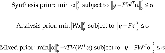
Most previous works in MR image reconstruction used either the synthesis prior or the mixed prior. In a previous work, we proposed the analysis prior optimization for MR image reconstruction [21]. The problem with such disparate studies is that during practical MR image reconstruction, one does not know which reconstruction algorithm will produce the best possible result. Thus, there is a need to evaluate all these algorithms on a uniform dataset. In this chapter, we compare the three different priors on real MR images in order to ascertain which prior yields the best possible results.

18.3.1.1 Experimental Evaluation

The results in this section have been reproduced from [23], where we performed an experimental study on three different MR images (Figure 18.1). The ground-truth data are collected by fully sampling the k-space on a uniform Cartesian grid. All the images are of size 256 × 256 pixels. The T2-weighted brain and the phantom data have been obtained from [18]. These data were collected by a 1.5 T scanner with echo time of 85 ms. The T2-weighted rat's spinal cord was acquired by a 7 T scanner at UBC MRI Lab with echo time of 13 ms. For all the images, spin echo sequence was used. We simulated Cartesian undersampling (where lines in the vertical direction randomly are omitted [16]).

In our experiments, the number of vertical lines for Cartesian sampling was fixed at 96. This corresponds to a sampling ratio of 37.5% (acceleration factor of 2.7) for Cartesian sampling. For Cartesian sampling, 33% of the samples were collected from the center of the k-space, while the rest was randomly collected from the remaining k-space. We ran the experiments on different values of p between zero and one for the three types of prior and found that on an average, the best results are obtained for p = 0.8.

The Haar wavelets have been used as the sparsifying transform. The synthesis prior and the analysis prior algorithm yielded the same answer for orthogonal wavelets. For redundant wavelet transform, the synthesis prior yielded worse results than the orthogonal wavelet transform, but the analysis prior with redundant wavelet transform gave better results. The same phenomenon had been observed in previous studies [21]. Therefore, for the synthesis prior and the mixed prior (which is a combination of synthesis and TV prior), the orthogonal Haar transform was used only; for the analysis prior, the redundant Haar transform is used.

For quantitative evaluation, the normalized mean squared error (NMSE) was used for comparing the results in Table 18.1.

NMSE values do not speak about the image quality. Therefore, for qualitative evaluation, we show the reconstructed images and the difference images in Figure 18.2. The difference images have been magnified five times for visual clarity.

Images

FIGURE 18.1
(a) Rat (spine), (b) brain, and (c) phantom.

TABLE 18.1
Reconstruction Accuracy for Cartesian Undersampling (p = 0.8)

Image Name	Synthesis Prior Orthogonal Haar	Mixed Prior	Analysis Prior Redundant Haar
Rat	0.1244	0.0955	0.0675
Brain	0.1830	0.1165	0.0709
Phantom	0.3409	0.2321	0.1847

From Figure 18.2, it is easily discernible that the analysis prior optimization yields visually superior images compared to the others. In all the images, the reconstruction artifacts are blocky; this is because the Haar wavelets have been used as the sparsifying transform.

A more detailed comparative study on this topic can be found in [23].

18.3.2 Modeling the MR Image as a low-Rank Matrix

From the discussion in Section 18.2, we see that it is possible to solve for a vector of size n from its lower-dimensional projections (m) provided the number of nonzero entries in the vector s is sufficiently small (18.4). A n dimensional vector with s nonzero elements has only 2s (s positions and corresponding s values) degrees of freedom. CS is able to find a solution when the number of measurements is sufficiently larger than the degrees of freedom in the solution. The same idea applies to low-rank matrix recovery from undersampled projections. A matrix of size N x N but of rank r has only r(2n − r) degrees of freedom. As long as the number of lower-dimensional projections is suffi-ciently larger than the number of degrees of freedom, it is possible to recover the matrix.

In this section, we show that transform domain sparsity is not the only way the information content of the image is compactly captured. In many cases, singular value decomposition (SVD) can also efficiently represent the information content of the MR image. Therefore, instead of using CS for recovering the matrix from undersampled k-space measurements, it is possible to exploit the low-rank property of the images to recover them.

Owing to the spatial redundancy, MR images do not have full rank, i.e., for an image of size N × N, its rank is r < N. For an image of rank “r,” the number of degrees of freedom is r(2N − r). Thus, when r ≪ N, the number of degrees of freedom is much less than the total number of pixels N². This idea has been successfully used in recent studies to propose SVD-based compression schemes for images [24,25]. Just as CS exploits sparsity in the transform domain to reconstruct the MR image from subsampled k-space data, this approach will exploit the low-rank property of the medical images for their reconstruction.

Images

FIGURE 18.2
Reconstructed and difference images for Cartesian undersampling. For all the rows: left image—synthesis prior, middle image—mixed prior, and right image—analysis prior. Odd rows represent the reconstructed images, and the even rows represent difference images.

Images

The image can be recovered from its subsampled k-space measurements by exploiting its rank deficiency in the following manner:

\min r a n k (X) subject to {‖ y - F x ‖}_{2}^{2} \leq σ (18.15)

$\min r a n k (X) subject to {‖ y - F x ‖}_{2}^{2} \leq σ (18.15)$

where

X is the image

x is the vectorized version of the image

As in l₀-norm minimization, the rank minimization problem (18.15) is NP hard. In CS, the NP hard problem is bypassed by replacing the l₀-norm by its nearest convex surrogate—the l₁-norm. Similarly for (18.15), it is intuitive to replace the NP hard objective function of rank minimization by its tightest convex relaxation—the nuclear norm. Therefore, in [30], we have proposed to solve the following problem instead:

\min {‖ X ‖}_{*} subject to {‖ y - F x ‖}_{2}^{2} \leq σ (18.16)

$\min {‖ X ‖}_{*} subject to {‖ y - F x ‖}_{2}^{2} \leq σ (18.16)$

where ‖X‖_* is the nuclear norm of the image X, which is defined as the sum of its singular values.

The fact that the rank of the matrix can be replaced by its nuclear norm for optimization purpose is justified theoretically as well. Recent theoretical studies by Recht et al. [26–28] and others [29] show the equivalence of (18.15) and (18.16). We refrain from theoretical discussion on this subject and ask the interested reader to peruse References [25–29].

The work [30] is motivated by the efficacy of l_p-norm minimization in non-convex CS. The actual problem in CS is to solve the l₀-norm minimization problem (18.2). This problem being NP hard is replaced by its closest convex surrogate the l₁-norm (18.3). The l₁-norm minimization problem is more popular in CS because its envelope is convex and therefore easier to theoretically analyze. However, the l_p-norm better approximates the original NP hard problem. Consequently, it gives better results [12,20,22,23] both theoretically and practically.

In the aforesaid work [30], our main target was to solve the NP hard rank minimization problem (18.15). But following previous studies in CS, we propose to replace the NP hard rank minimization problem by its closest non-convex surrogate the Schatten-p-norm instead of the convex nuclear norm. The Schatten-p-norm is defined as

{‖ X ‖}_{p *} = \sum_{i} σ_{i}^{p}, where σ_{i}' s are singular values of X (18.17)

${‖ X ‖}_{p *} = \sum_{i} σ_{i}^{p}, where σ_{i}' s are singular values of X (18.17)$

In [30], we proposed to solve the MR image reconstruction problem by mini-mizing its Schatten-p norm directly. Mathematically, the optimization problem is as follows:

\min {‖ X ‖}_{p *} subject to {‖ y - F x ‖}_{2}^{2} \leq σ (18.18)

$\min {‖ X ‖}_{p *} subject to {‖ y - F x ‖}_{2}^{2} \leq σ (18.18)$

Before our work [30], there was no existing algorithm to solve the Schatten-p-norm minimization problem. For the first time, we proposed an efficient algorithm to solve this problem (18.18) in [30]. The interested reader should refer to the aforementioned reference for the algorithm.

18.3.2.1 Experimental Evaluation

We carried out the experiments on three slices from the BrainWeb (two slices) and National Institute of Health (NIH) (one slice) databases (see Figure 18.3). Radial sampling was employed to collect the k-space data. Our proposed reconstruction technique is compared against the standard CS-based reconstruction method called the CSMRI [18]. One of the fastest known l₁-norm minimization algorithms called the spectral projected gradient L1 (SPGL1) [31] was used as the solver from CSMRI. The Haar wavelet is used as the sparsifying transform for CSMRI. Our proposed reconstruction approach, based on Schatten-p-norm minimization, gave the best results when the value of p is 0.9. Therefore, for all the experiments, we kept the fixed p at the said value.

Images

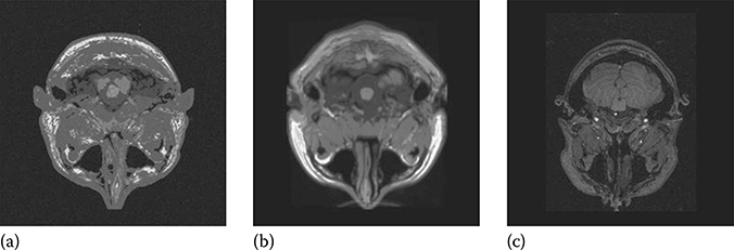
FIGURE 18.3
Ground-truth images: (a) BrainWeb new, (b) BrainWeb old, and (c) NIH.

We will provide both quantitative and qualitative reconstruction results. As in the previous section for quantitative comparison, the NMSE between the reconstructed image and the ground truth is computed. However, we also provide the reconstructed images for qualitative assessment.

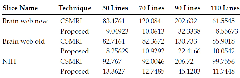
In the first set of experiments, it is assumed that the data are noise free. The number of radial sampling lines has been varied from 50 to 110 in steps of 20. In Table 18.1, the NMSE values are shown, and in Table 18.2, the reconstruction times are tabulated.

Table 18.2 shows that for the BrainWeb new and the NIH data, the reconstruction error from our proposed method is slightly higher (1%–2%) and for the BrainWeb old data, the error is slightly lower (around 1%) than CSMRI. However, these slight variations are practically indistinguishable in the reconstructed images. The reconstructed images from the proposed approach and CSMRI are shown in Figure 18.4 for visual quality assessment.

In the following table, we compare the reconstruction times required for our proposed method and by the CS-based method.

TABLE 18.2
Comparison of NMSE for Proposed and CS Reconstruction

Images

FIGURE 18.4
Reconstruction results (220 lines). (a) CSMRI reconstruction and (b) reconstruction from proposed approach. Left to right—BrainWeb new, BrainWeb old, and NIH.

Table 18.3 shows that our proposed approach is about 5–10 times faster than CSMRI. It must be remembered that the SPGL1 is one of the most sophisticated and fastest l₁-norm minimization algorithms where our algorithm has been implemented naively. The core computational demand of our algorithm is in computing the SVD in each iteration. Computing the SVD naively is time consuming since we already know that the matrix is rank deficient. Our current algorithm can be made even faster by employing PROPACK [32] for computing the SVD.

TABLE 18.3
Comparison of Reconstruction Times

Images

CS-based MR image reconstruction techniques have been successful in reconstructing image from subsampled k-space measurements. Our proposed low-rank model of the MR image aims at the same goal but from an entirely new perspective. The reconstruction results show that the proposed approach and the CS-based techniques provide virtually indistinguishable results. However, the low-rank model has a distinct advantage in terms of speed. It is about 5–10 times faster than one of the fastest CS-based reconstruction algorithms.

18.4 Accelerating Multichannel Scans

The objective of multicoil parallel MRI is to reduce the data acquisition time. Instead of scanning the whole k-space by a single receiver coil, parallel MRI uses multiple coils. Depending on the physical position of the receiver coils in the scanner, they have different field of views and thereby different sensitivity profiles/maps. Acceleration is achieved since each of the receiver coils partially samples the k-space. The sampling mask used to undersample the k-space is the same for all the coils. The ratio of the total number of possible k-space samples to the number of samples actually collected by each coil is the “acceleration factor.” In parallel MRIs, the problem is to reconstruct the underlying MR image given the partial k-space samples acquired by each coil.

Mathematically, the multicoil data acquisition process can be formulated as

y_{i} = R F S_{i} x + η_{i}, i = 1 \dots C (18.19)

$y_{i} = R F S_{i} x + η_{i}, i = 1 \dots C (18.19)$

where

y_i is the k-space data collected by the ith coil

F is the Fourier transform operator

R is the undersampling mask

S_i is the sensitivity map of the ith coil

x is the image to be reconstructed (vectorized image consisting of q pixels)

η is the noise (a complex vector of length p)

In Equation 18.19, the image to be reconstructed x and the sensitivity maps S_i’s are the unknowns. The basic parallel MR image reconstruction techniques—sensitivity encoding (SENSE) [33] and simultaneous acquisition of spatial harmonics (SMASH) [34]—explicitly require the sensitivity maps to be available. More recent techniques like generalized autocalibrating partially parallel acquisitions (GRAPPA) [35] estimate the sensitivity-dependent interpolation weights from the autocalibration signal (ACS) lines.

If the sensitivity maps are available, then SENSE is physically the most optimal reconstruction technique in terms of mean squared error. It is based on solving the following inverse problem:

y = R F S x + η (18.20)

$y = R F S x + η (18.20)$

where

$\begin{matrix} y = [\begin{matrix} y_{1} \\ \dots \\ y_{C} \end{matrix}] \\ S = [\begin{matrix} S_{1} \\ \dots \\ S_{1} \end{matrix}] \\ η = [\begin{matrix} η_{1} \\ \dots \\ η_{C} \end{matrix}] \end{matrix}$ $\begin{matrix} y = [\begin{matrix} y_{1} \\ \dots \\ y_{C} \end{matrix}] \\ S = [\begin{matrix} S_{1} \\ \dots \\ S_{1} \end{matrix}] \\ η = [\begin{matrix} η_{1} \\ \dots \\ η_{C} \end{matrix}] \end{matrix}$

R and F carry their predefined meanings.

Estimating the sensitivity maps is not trivial. The accuracy of image reconstruction is sensitive to the accuracy with which the sensitivity maps have been computed. But even with this shortcoming, SENSE is by far the most widely used parallel MR image reconstruction technique. All commercial scanners use modifications of the basic SENSE method—Philips uses SENSE, Siemens uses mSENSE, General Electric uses ASSET, and Toshiba uses SPEEDER [36].

In the section, we will discuss the basic SENSE method and its advancements in recent times based on CS techniques. In recent times, some robust SENSE algorithms have been developed that are less sensitive to the estimated sensitivity maps compared to the previous ones. In the next section, we discuss a technique that enjoys the same mathematical rigor as SENSE but does not require sensitivity map estimation either implicitly or explicitly. This is by far the most robust multicoil reconstruction algorithm that can achieve better reconstruction results than commercial and state-of-the-art algorithms in parallel MRI.

18.4.1 SENSE-based Reconstruction

The physical data acquisition model for the multicoil parallel MRI is expressed by Equation 18.20. In SENSE, it is assumed that the coil sensitivities are known, i.e., S is given. The first study that proposed the SENSE framework [33] solves the reconstruction problem by the least squares optimization:

\min_{x} {‖ y - R F S x ‖}_{2} (18.21)

$\min_{x} {‖ y - R F S x ‖}_{2} (18.21)$

However, in practical scenarios, a regularized version of the least squares problem is solved [37–39]:

\min_{x} {‖ y - R F S x ‖}_{2} + λ Φ (x) (18.22)

$\min_{x} {‖ y - R F S x ‖}_{2} + λ Φ (x) (18.22)$

where

Φ(x) is the regularization term

λ is the regularization parameter

The regularization function Φ can be the l₁-norm of the wavelet transform of the image; it can also be an isotropic or anisotropic TV of the image.

Recently, CS-based techniques have been incorporated into the SENSE framework [40]. The reconstruction problem is formulated as

\underset{x}{\arg \min} {‖ Ψ x ‖}_{1} subject to {‖ y - R F S x ‖}_{2} \leq ε (18.23)

$\underset{x}{\arg \min} {‖ Ψ x ‖}_{1} subject to {‖ y - R F S x ‖}_{2} \leq ε (18.23)$

This formulation (18.23) is named SparSENSE. Instead of incorporating the sparsity of the image in the transform domain, the information regarding the rank deficiency of the image matrix can also be used in the SENSE framework. This leads to the following nuclear norm-regularized SENSE reconstruction (NNSENSE) problem [41]:

\underset{x}{\arg \min} {‖ X ‖}_{*} subject to {‖ y - R F S x ‖}_{2} \leq ε (18.24)

$\underset{x}{\arg \min} {‖ X ‖}_{*} subject to {‖ y - R F S x ‖}_{2} \leq ε (18.24)$

Here, ‖X‖_* is the nuclear norm of the image matrix. It is the sum of the singular values of X. This is a convex metric and is a special case of the Schatten-p-norm where p equals 1.

All the aforementioned studies assume that the sensitivity maps are known. Thus, the accuracy of the reconstruction technique depends on the provided sensitivity maps. However, the estimates of the sensitivity maps are not always accurate. In order to get a robust reconstruction, a joint estimation of the image and sensitivity map has been proposed in JSENSE [42]. The sensitivity map for each coil is parameterized as a polynomial of degree N whose coefficient is a. The SENSE equation (18.20) is expressed as

y = R F S (a) x + η (18.25)

$y = R F S (a) x + η (18.25)$

where the sensitivity for the ith coil at position (m,n) is given by $s_{i} (m, n) = \sum_{p = 0}^{N} \sum_{q = 0}^{N} a_{i, p, q} x^{p} y^{q}$ $s_{i} (m, n) = \sum_{p = 0}^{N} \sum_{q = 0}^{N} a_{i, p, q} x^{p} y^{q}$ , where (m,n) denotes the position and N and a denote the degree of the polynomial and its coefficients, respectively.

In order to jointly estimate the coil sensitivities (given the polynomial formulation) and the image, the following problem has to be solved:

\underset{a, x}{\arg \min} {‖ y - R F S (a) x ‖}_{2} (18.26)

$\underset{a, x}{\arg \min} {‖ y - R F S (a) x ‖}_{2} (18.26)$

However, it has been argued in [42] that solving for all the variables jointly is an intractable nonconvex problem; hence, the image and the polynomial coefficients were solved iteratively, as follows:

\underset{x}{\arg \min} {‖ y - R F S (a) x ‖}_{2} (18.27)

$\underset{x}{\arg \min} {‖ y - R F S (a) x ‖}_{2} (18.27)$

In (18.27), it is assumed that the coil sensitivity parameters (a) are given, and the problem is to solve for the image x. In the next step, it is assumed that the image x is given, and based on that, the coil sensitivity parameters a are estimated:

\underset{a}{\arg \min} {‖ y - R F S (a) x ‖}_{2} (18.28)

$\underset{a}{\arg \min} {‖ y - R F S (a) x ‖}_{2} (18.28)$

Problem (18.26) is nonconvex, and there is no guarantee that solving it by iterating between (18.27) and (18.28) will converge. However, with reasonably good initial estimates of the sensitivity maps, JSENSE provides considerable improvement over SENSE reconstruction.

The JSENSE was regularized using the CS framework [43]. It was assumed that the image is sparse in a finite difference domain and the coil sensitivity is sparse in Chebyshev polynomial basis or in Fourier domain. Therefore, it is proposed in [43] to solve the problem by alternately solving the following two optimization problems:

\hat{x} = \min_{x} {‖ y - R F S (a) x ‖}_{2} + λ_{x} T V (x) (18.29)

$\hat{x} = \min_{x} {‖ y - R F S (a) x ‖}_{2} + λ_{x} T V (x) (18.29)$

\hat{S} = \min_{x} {‖ y - R F X s ‖}_{2} + λ_{s} Ψ {‖ s ‖}_{1} (18.30)

$\hat{S} = \min_{x} {‖ y - R F X s ‖}_{2} + λ_{s} Ψ {‖ s ‖}_{1} (18.30)$

where Ψ is the Chebyshev polynomial basis.

In (18.29), the image is solved by TV regularization assuming the sensitivity map is known. In (18.30), the sensitivity map is estimated assuming the image is known. Here, Ψ is the sparsifying basis (Chebyshev polynomial basis or Fourier basis) for the sensitivity maps.

The problem with this formulation is that the basis used for sparsifying the sensitivity maps and the measurement basis is not incoherent. This violates the basic premises of CS-based reconstruction [44] and thus does not yield good reconstruction results.

To overcome the problem of modeling the sensitivity maps as a sparse set of Fourier coefficients, we propose an alternate model in this chapter. We propose to model the sensitivity maps as rank-deficient matrices. This is a new assumption. In order to corroborate it empirically, we show plots of singular value decay of the two sensitivity maps (one and three) for an 8-channel MRI scanner in Figure 18.5a. It shows that the singular values of the sensitivity maps decay fast and thus the sensitivity maps are approximately rank deficient.

The MR image can be either modeled as a sparse set of transform coefficients or modeled as a rank-deficient matrix [30,41]. In this chapter, we propose modeling the sensitivity maps as rank-deficient matrices. Assuming that the image is sparse in a transform domain, the parallel MRI problem can be formulated as follows:

Images

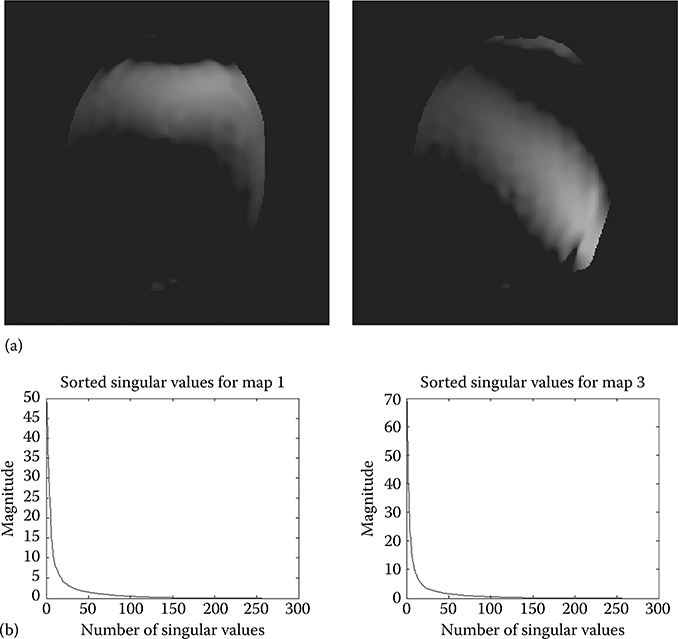
FIGURE 18.5
(a) Sensitivity maps and (b) decay of singular values.

\begin{array}{l} \min_{x, S} {‖ y - R F S x ‖}_{2} subject to \\ {‖ W x ‖}_{1} + γ T V (x) \leq τ_{1} \\ {‖ S_{i} ‖}_{*} \leq τ_{2}, \forall i \end{array} (18.31)

$\begin{array}{l} \min_{x, S} {‖ y - R F S x ‖}_{2} subject to \\ {‖ W x ‖}_{1} + γ T V (x) \leq τ_{1} \\ {‖ S_{i} ‖}_{*} \leq τ_{2}, \forall i \end{array} (18.31)$

where

τ₁ and τ₂ are the constraints on the transform domain sparsity of the image and on the rank deficiencies of the sensitivity maps, respectively

γ is the term balancing the relative importance of the transform domain sparsity and TV

Alternately, when the image is modeled as a rank-deficient matrix, one would ideally solve the following problem:

\begin{array}{l} \min_{x, S} {‖ y - R F S x ‖}_{2} subject to \\ {‖ X ‖}_{*} \leq τ_{1} \\ {‖ S_{i} ‖}_{*} \leq τ_{2}, \forall i \end{array} (18.32)

$\begin{array}{l} \min_{x, S} {‖ y - R F S x ‖}_{2} subject to \\ {‖ X ‖}_{*} \leq τ_{1} \\ {‖ S_{i} ‖}_{*} \leq τ_{2}, \forall i \end{array} (18.32)$

where τ₁ represents the constraint on the rank deficiency of the MR image to be reconstructed.

Unlike [43], we exploit the rank deficiency of the sensitivity maps in order to estimate them. The incoherency criterion required by CS-based techniques does not arise in our formulation. The proposed method is called iSENSE.

Both (18.31) and (18.32) are nonconvex problems similar to the JSENSE formulation. Solving for the MR image and the sensitivity maps jointly is an intractable problem. Following the approach in JSENSE, we propose to iteratively solve the optimization problems by the following algorithm.

Algorithm 1

Initialize: Use an initial estimate of the sensitivity maps.

Iteratively solve steps 1 and 2 until convergence.

Step 1: Using the initial or the estimated sensitivity maps obtained in step 2, solve for the image either by solving a CS problem

\min_{x} {‖ y - R F S x ‖}_{2} subject to {‖ W x ‖}_{1} + γ T V (x) \leq τ_{1}

$\min_{x} {‖ y - R F S x ‖}_{2} subject to {‖ W x ‖}_{1} + γ T V (x) \leq τ_{1}$

or by solving nuclear norm minimization

\min_{x} {‖ y - R F S x ‖}_{2} subject to {‖ X ‖}_{*} \leq τ_{1}

$\min_{x} {‖ y - R F S x ‖}_{2} subject to {‖ X ‖}_{*} \leq τ_{1}$

Step 2: Using the estimate of the image from Step 1, solve for the sensitivity maps by the nuclear norm minimization:

\min_{S} {‖ y - R F S x ‖}_{2} subject to {‖ S_{i} ‖}_{*} \leq τ_{2}, \forall i

$\min_{S} {‖ y - R F S x ‖}_{2} subject to {‖ S_{i} ‖}_{*} \leq τ_{2}, \forall i$

There are two issues with Algorithm 1—(i) There are no efficient solvers for the stated CS or nuclear norm minimization problems; (ii) it is not an easy task to specify values for τ₁ and τ₂. This is because obtaining estimates on the sparsity of the image or the rank deficiencies of image and the sensitivity maps is very difficult. Both these issues can be resolved by solving the opti-mization problems in an equivalent alternative form where the constraint is on the data fidelity term instead of on the sparsity or rank deficiency. This leads to the following algorithm.

Algorithm 2

Initialize: An initial estimate of the sensitivity maps.

Iteratively solve steps 1 and 2 until convergence.

Step 1: Using the initial or the estimated sensitivity maps obtained in step 2, solve for the image either by solving a CS problem

\min_{x} {‖ W x ‖}_{1} + γ T V (x) subject to {‖ y - R F S x ‖}_{2} \leq ε_{1}

$\min_{x} {‖ W x ‖}_{1} + γ T V (x) subject to {‖ y - R F S x ‖}_{2} \leq ε_{1}$

or by solving nuclear norm minimization

\min_{x} {‖ X ‖}_{*} subject to {‖ y - R F S x ‖}_{2} \leq ε_{1}

$\min_{x} {‖ X ‖}_{*} subject to {‖ y - R F S x ‖}_{2} \leq ε_{1}$

Step 2: Using the estimate of the image from Step 1, solve for the sensitivity maps by nuclear norm minimization:

\min_{S} {‖ S_{i} ‖}_{*} subject to {‖ y - R F S x ‖}_{2} \leq ε_{1}, \forall i

$\min_{S} {‖ S_{i} ‖}_{*} subject to {‖ y - R F S x ‖}_{2} \leq ε_{1}, \forall i$

Algorithm 2 requires solving CS and nuclear norm minimization problems. Efficient algorithms are available for both of them. It should be noted that Step 1 (which assumes that the sensitivity maps are given) is the same as SparSENSE or NNSENSE as the case may be.

The problems (18.31) and (18.32) are nonconvex. Hence, their solution is not guaranteed to reach a unique minimum. Therefore, it is not possible to theoretically analyze convergence of Algorithm 2. For similar reasons, previous studies [42,43] did not analyze the convergence of iterative SENSE algorithms. However, in this work, we found that practically the said algorithm converges in three iterations.

18.4.1.1 Experimental Evaluation

All the experiments were performed on a 64 bit AMD Athlon processor with 4 GB of RAM running Windows 7. The simulations were carried out on MATLAB^® 2009.

There are five sets of ground-truth data used for the experimental evaluation (Figure 18.6). The brain data have been used previously in [19]. The brain data come from a fully sampled T1-weighted scan of a healthy volunteer. The volunteer was scanned using spoiled gradient echo sequence with the following parameters—echo time = 8 ms, repetition time = 17.6 ms, and flip angle = 20°. The scan was performed on a GE Signa EXCITE 1.5 T scanner, using an eight-channel receiver coil. The eight-channel data for Shepp–Logan phantom were simulated using the B1 simulator (http://maki.bme.ntu.edu.tw/tool_b1.html) using the default settings for eight-channel receiver coil. The UBC MRI Lab prepared three datasets. The first one is a phantom created by doping saline with Gd-DTPA. The second and third ones are the ex vivo and in vivo images of a rat's spinal cord. A four-coil Bruker scanner was used for acquiring the data using a FLASH sequence. The ground truth has been formed by sum-of-squares reconstruction of the multichannel images. All the images had a native resolution of 256 × 256 pixels.

This method only requires an initial estimate of the sensitivity maps. For this reason, we have used the simple sum-of-squares method for sensitivity estimation [33,42]. The initial sensitivity maps were computed in the following manner:

• For each coil, the center of the k-space of the image was fully sampled (ACS lines). One-third of all the lines were used as ACS lines. The central k-space region was apodized by a Kaiser window of parameter 4 [42].

Images

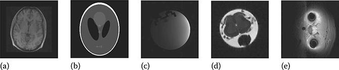
FIGURE 18.6
Ground-truth images: (a) brain, (b) Shepp–Logan phantom, (c) UBC phantom, (d) rat ex vivo, and (e) rat in vivo.

• The corresponding low-frequency images were computed by using the 2D inverse Fourier transform.

• The low-frequency images for each coil were normalized by dividing them by the sum-of-squares image. These were used as the initial estimates of sensitivity maps.

Our method needs only two parameters (∊₁ and ∊₂ in Algorithm 2) to be specified; the values of ∊₁ and ∊₂ had been fixed at 1 and 10, respectively. The choice behind the particular parametric values can be understood intuitively. From previous studies, it is known that by using CS-based and nuclear norm regularization-based techniques, it is possible to estimate the image to a high degree of accuracy. Therefore, while estimating the image, the data fidelity term (∊₁) is fixed at a small value. But estimating the sensitivity map to a high degree of accuracy is difficult. For this reason, the data fidelity term (∊₂) during sensitivity map estimation is fixed at a larger value (compared to ∊₁).

In [45], it is argued that the sensitivity maps should be normalized by their combined sum-of-squares map. The proposed iSENSE method models the sensitivity maps as rank-deficient matrices; thus, the estimated sensitivity maps are not normalized. During actual implementation, once the sensitivity maps are estimated, they are normalized by their sum-of-squares map before being used for image estimation.

We have compared our proposed iSENSE method with state-of-the-art reconstruction techniques like SparSENSE [41] and the NNSENSE [40] and a well-known traditional reconstruction technique GRAPPA [35]. All these are single-pass methods and assume either implicitly (GRAPPA) or explicitly (SparSENSE and NNSENSE) the knowledge of sensitivity maps. We also compared our work against the recently developed technique of JSENSE [42]. JSENSE alternately estimates the MR image and the sensitivity maps and is similar in spirit to our proposed iSENSE.

It must be noted that SparSENSE and NNSENSE are actually Step 1 of our proposed algorithm. We found that our proposed iSENSE converges in three iterations; after which, there is no significant improvement in results.

In this work, we simulate a variable density subsampling scheme where the center of the k-space is fully sampled, while the rest of the k-space is sampled sparsely. The k-space is fully sampled along the frequency encoding (x-axis) direction but is undersampled along the phase encoding direction. For the eight-channel data (brain and Shepp–Logan phantom), the acceleration factor is 4, while for the four-channel data (UBC MRI slices 1 and 7), the acceleration factor is 2. The dense sampling of the center of k-space is required for estimating the sensitivity maps.

First, we show the quantitative experimental results. The measurement for reconstruction accuracy is NMSE between the ground-truth image formed by sum-of-squares reconstruction from the fully sampled k-space data and the magnitude image obtained by reconstruction (by various techniques) from partially sampled k-space data. For our proposed method iSENSE, iSENSE CS denotes the case where the image reconstructed by SparSENSE and iSENSE NN denotes the case where image is reconstructed by NNSENSE.

TABLE 18.4
iSENSE Reconstruction Accuracy after 1st, 2nd, and 3rd Iterations

Images

The reconstruction accuracy from our proposed method iSENSE is shown in Table 18.4. The results are shown for all three iterations.

Next, we compare our proposed technique iSENSE against the methods mentioned earlier. It has been reported in [42] that the JSENSE method converges in three to four iterations. We ran the JSENSE algorithm for four iterations; the reconstruction accuracy after the final iteration is reported. It must be noted that after the first iteration of iSENSE, the obtained result corresponds to SparSENSE (for the CS-based technique) and NNSENSE (for the nuclear norm regularization-based technique).

The numerical results indicate that our proposed iSENSE method is better than the techniques compared against, at least for the datasets used in this work. However, the NMSE is not always the best metric for reconstruction accuracy. Table 18.5 shows that in terms of NMSE, JSENSE is almost as accurate as our proposed iSENSE CS and iSENSE NN for all the datasets and GRAPPA has similar reconstruction accuracy as our proposed iSENSE methods for the brain, Shepp–Logan phantom, and the UBC MRI phantom. We will show in Figures 18.9 through 18.12 that in terms of qualitative reconstruction, our proposed method gives considerably better results than JSENSE and GRAPPA.

TABLE 18.5
Comparison of Reconstruction Accuracy from Various Techniques

Images

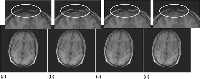
FIGURE 18.7
Brain images reconstructed by iSENSE CS: (a) after 1st iteration (SparSENSE), (b) after 2nd iteration, (c) after 3rd (final) iteration, and (d) ground truth.

Before comparing iSENSE with JSENSE and GRAPPA, we will show the benefit of iSENSE reconstruction. Especially for clinical MRI, one is interested in preserving minute anatomical details. This is evident from Figures 18.7 and 18.8. Here, we show, for the brain image, how the fine anatomical details are recovered after each iteration of our proposed iSENSE technique.

The first image (a) shows the reconstructed image after Step 1. This image (a) corresponds to SparSENSE (Figure 18.7 and NNSENSE (Figure 18.8). The second image (b) shows the reconstructed image after two iterations, i.e., Step 1 → Step 2 → Step 1. The third image (c) shows the reconstructed image after three iterations, i.e., Step 1 → Step 2 → Step 1 → Step 2 → Step 1. There is no significant improvement after the third iteration. The fourth image (d) is the ground-truth image.

Images

FIGURE 18.8
Brain images reconstructed by iSENSE NN: (a) after 1st iteration (NNSENSE), (b) after 2nd iteration, (c) after 3rd (final) iteration, and (d) ground truth.

The top portion of each image has been magnified for better clarity. It is easy to see from the magnified portions that in the SparSENSE and NNSENSE reconstruction, some fine anatomical details are missing (encircled area). After the second iteration, some of the details are captured. The third iteration shows slight improvement over the second iteration. By the third iteration, the anatomical detail captured is as good as the ground truth.

Quantitative results in Table 18.5 do not give a clear idea regarding the qualitative aspects of reconstruction. In Figures 18.9 through 18.12, it is shown how the iSENSE method fairs over GRAPPA and JSENSE. We show the reconstructed and difference images for the real datasets (brain, UBC MRI phantom, rat ex vivo, rat in vivo). The difference images are computed by taking the absolute difference between the ground-truth and the reconstructed magnitude image. The difference images have been magnified 10 times for visual clarity.^* The reconstruction results from iSENSE CS and iSENSE NN are almost similar. They do not have any quantitative or discernible differences. In this work, we therefore show the results from iSENSE CS only. We show the results for iSENSE CS, JSENSE, and GRAPPA, since the reconstruction results for SparSENSE and NNSENSE have already been shown in Figures 18.7 and 18.8.

Images

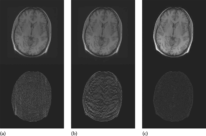
FIGURE 18.9
Reconstructed (1st row) and difference (2nd row) images of brain. (a) GRAPPA, (b) JSENSE, and (c) iSENSE.

Images

FIGURE 18.10
Reconstructed (1st row) and difference (2nd row) images of UBC MRI phantom 1. (a) GRAPPA, (b) JSENSE, and (c) iSENSE.

Images

FIGURE 18.11
Reconstructed (1st row) and difference (2nd row) images of rat ex vivo 1. (a) GRAPPA, (b) JSENSE, and (c) iSENSE.

Images

FIGURE 18.12
Reconstructed (1st row) and difference (2nd row) images of rat in vivo 1. (a) GRAPPA, (b) JSENSE, and (c) iSENSE.

Both GRAPPA and JSENSE reconstruction methods show visible aliasing artifacts for all the images. This is especially discernible from the difference images. Our proposed iSENSE yields the best reconstruction results for all the images with very little reconstruction artifacts (the difference image is almost dark in all cases).

In most cases, the reconstruction times for static MRI reconstruction are not at a premium. However, it is worthwhile to compare the speed of the reconstruction algorithms especially when the iSENSE NN gives about an order of improvement in speed over the iSENSE CS-based method. The reconstruction times are shown in Table 18.6. The results reported here are at par with results from previous studies [30,41], where it was shown that NN regularization yields about an order of magnitude faster reconstruction compared to CS-based techniques.

TABLE 18.6
Reconstruction Times (Rounded in Seconds) for iSENSE CS and iSENSE NN

Images

Both the methods iSENSE CS and iSENSE NN recover images with high accuracy in terms of quantitative and qualitative evaluation. However, given the present challenges of using low-rank techniques in 3D reconstruction, the CS-based reconstruction technique is more practical.

18.4.2 Calibration-Free Parallel MRI Reconstruction

All previous multicoil parallel MR image reconstruction algorithms require some form of parameter estimation pertaining to the sensitivity profiles. The image domain methods require the estimate of the sensitivity profiles from the calibration data, while the frequency domain methods require computing the linear interpolation weights from the calibration data. In both cases, the assumption is that the estimates based on the calibration data should hold for the unknown image (to be reconstructed) as well. For image domain methods, there are different ways to compute the sensitivity profiles, and the reconstruction results are dependent on the technique used to compute them. For frequency domain methods, besides the calibration data, the interpolation weights also depend on the calibration kernel. In short, all known methods for multicoil parallel MRI are dependent on their respective parameter estimation stage. In the section on Experimental Evaluation, we will show that the well-known image domain and frequency domain methods are indeed sensitive to the results of the calibration stage.

In order to alleviate the sensitivity issues associated with calibration, we propose a solution that does not require calibration in any form. Our method is named CaLM (Calibration-Less Multicoil) MRI [55].

We rewrite the physical data acquisition model (18.19) for multicoil MRI:

y_{i} = R F S_{i} x + η_{i}, i = 1 \dots C

$y_{i} = R F S_{i} x + η_{i}, i = 1 \dots C$

This can be expressed in a slightly different fashion as

y_{i} = R F x_{S_{i}} + η_{i}, i = 1 \dots C (18.33)

$y_{i} = R F x_{S_{i}} + η_{i}, i = 1 \dots C (18.33)$

where $x_{S_{i}} = S_{i} x$ $x_{S_{i}} = S_{i} x$ are the sensitivity-encoded images for each coil.

Incorporating the wavelet transform into (18.33), we get

y_{i} = R F W^{T} α_{S_{i}} + η_{i}, i = 1 \dots C (18.34)

$y_{i} = R F W^{T} α_{S_{i}} + η_{i}, i = 1 \dots C (18.34)$

In compact matrix–vector notation, (18.34) can be expressed as

y = E_{W} α_{S} + η (18.35)

$y = E_{W} α_{S} + η (18.35)$

where

y = [\begin{matrix} y_{1} \\ \dots \\ y_{C} \end{matrix}], E_{W} = [\begin{matrix} R F W^{T} & 0 & 0 \\ 0 & \dots & 0 \\ 0 & 0 & R F W^{T} \end{matrix}], α = [\begin{matrix} α_{S_{1}} \\ \dots \\ α_{S_{C}} \end{matrix}] and η = [\begin{matrix} η_{1} \\ \dots \\ η_{C} \end{matrix}]

$y = [\begin{matrix} y_{1} \\ \dots \\ y_{C} \end{matrix}], E_{W} = [\begin{matrix} R F W^{T} & 0 & 0 \\ 0 & \dots & 0 \\ 0 & 0 & R F W^{T} \end{matrix}], α = [\begin{matrix} α_{S_{1}} \\ \dots \\ α_{S_{C}} \end{matrix}] and η = [\begin{matrix} η_{1} \\ \dots \\ η_{C} \end{matrix}]$

Images

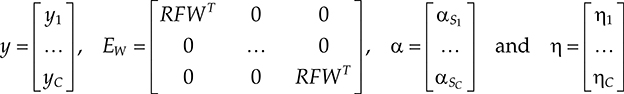
The problem is to solve the inverse problem (18.35). This is an underdeter-mined system of equations (the length of is $α_{S_{i}}$ $α_{S_{i}}$ the same as the total number of pixels in the image, but the length of y_i is less than the number of pixels as the k-space is undersampled) unlike SENSE or CS SENSE where the system is overdetermined. Thus, solving (18.35) requires the conditions of CS recovery to hold. These conditions are as follows:

The solution α_S is sparse in some sense.
The matrix E_W should follow the restricted isometric property (RIP) [23].

It is easy to argue that the α_S (wavelet coefficients) will be sparse. But we will argue that α_S will also be group sparse. In a group-sparse vector, all the coefficients are segregated into groups. Group sparsity means that in that vector, only a few groups will have nonzero coefficients, and the rest will be all zeros. Theoretically, group sparsity leads to stronger reconstruction accuracy compared to ordinary sparsity [46,47]. It is not possible to ensure that E_W will satisfy RIP. However, the sampling pattern can be designed to yield good results and will be discussed in the next subsection.

18.4.2.1 Group-Sparse Reconstruction

The wavelet transform encodes the discontinuities (singularities) in the images. The wavelet transform coefficients corresponding to the discontinuities are of high value, while those related to smooth areas are of low values (zero or near about zero). MR images are mostly smooth with a small number of discontinuities, and thus the wavelet coefficients of MR images are sparse.

In all previous parallel MRI studies, the underlying assumption was that the sensitivity profile is smooth. This is the reason why it can be computed from the low-frequency components of the k-space or by polynomial curve fitting. Since the sensitivity profile is smooth, it does not introduce jump discontinuities when it represents the underlying image; neither does it get rid of any existing discontinuities. Thus, the discontinuities that existed in the original MR image x also exist in the sensitivity-encoded images $x_{S_{i}}$ $x_{S_{i}}$ .

This does not imply that the levels of discontinuities in the sensitivity-encoded image would be the same as the original image, but the locations of the discontinuities will be the same. This in turn implies that the wavelet coefficients of the original image will be of similar values to those of the sensitivity-encoded images at corresponding positions; that is, if for a particular index the wavelet coefficient is large in the original MR image (x), then the wavelet coefficients of the sensitivity-encoded images $(x_{S_{i}})$ $(x_{S_{i}})$ will be high at the corresponding index. Similarly, for low-valued wavelet coefficients, the correspondence holds as well.

In summary, the wavelet coefficients corresponding to different sensitivity-encoded images will have similar values at corresponding positions/indices.

Now, the full wavelet coefficient vector α_S in (18.35) is usually expressed as

{\underset{α_{S_{1}}}{\underset{︸}{α_{S_{1}} (1), α_{S_{1}} (2), \dots, α_{S_{1}} (N)}} \underset{α_{S_{2}}}{\underset{︸}{α_{S_{2}} (1), α_{S_{2}} (2), \dots, α_{S_{2}} (N)}} \dots \underset{α_{S_{C}}}{\underset{︸}{α_{S_{C}} (1), α_{S_{C}} (2), \dots, α_{S_{C}} (N)}}}^{T} (18.36)

${\underset{α_{S_{1}}}{\underset{︸}{α_{S_{1}} (1), α_{S_{1}} (2), \dots, α_{S_{1}} (N)}} \underset{α_{S_{2}}}{\underset{︸}{α_{S_{2}} (1), α_{S_{2}} (2), \dots, α_{S_{2}} (N)}} \dots \underset{α_{S_{C}}}{\underset{︸}{α_{S_{C}} (1), α_{S_{C}} (2), \dots, α_{S_{C}} (N)}}}^{T} (18.36)$

where N is the total number of wavelet coefficients for each image. This wavelet coefficient vector α_S can also be grouped according to the position/index of the wavelet coefficients as follows:

{\underset{α (1)}{\underset{︸}{α_{S_{1}} (1), α_{S_{2}} (1), \dots, α_{S_{C}} (1)}} \underset{α (2)}{\underset{︸}{α_{S_{1}} (2), α_{S_{2}} (2), \dots, α_{S_{C}} (2)}} \dots \underset{α (N)}{\underset{︸}{α_{S_{1}} (N), α_{S_{2}} (N), \dots, α_{S_{C}} (N)}}}^{T} (18.37)

${\underset{α (1)}{\underset{︸}{α_{S_{1}} (1), α_{S_{2}} (1), \dots, α_{S_{C}} (1)}} \underset{α (2)}{\underset{︸}{α_{S_{1}} (2), α_{S_{2}} (2), \dots, α_{S_{C}} (2)}} \dots \underset{α (N)}{\underset{︸}{α_{S_{1}} (N), α_{S_{2}} (N), \dots, α_{S_{C}} (N)}}}^{T} (18.37)$

It is concluded that in (18.37), the coefficients in each of the groups (α(i)) will have similar values, i.e., the coefficients in any group will all be of high values or all be of very small values (zeroes or close to zero). In other words, α_S will be group sparse.

18.4.2.1.1 Synthesis Prior Formulation

The inverse problem (18.35) should be solved by taking into account the fact that the solution is group sparse. A group-sparse solution ${\hat{α}}_{S}$ ${\hat{α}}_{S}$ can be obtained by solving the following l_2,1 mixed-norm optimization problem [47–49]:

{\hat{α}}_{S} = \min_{α S} {‖ α_{S} ‖}_{2, 1} such that {‖ y - E_{W} α_{S} ‖}_{2}^{2} \leq σ (18.38)

${\hat{α}}_{S} = \min_{α S} {‖ α_{S} ‖}_{2, 1} such that {‖ y - E_{W} α_{S} ‖}_{2}^{2} \leq σ (18.38)$

where the l_2,1 mixed-norm is defined as ${‖ v ‖}_{2, 1} = {\sum_{j = 1}^{N} (\sum_{k = 1}^{C} v_{j}^{2} (k))}^{1 / 2}$ ${‖ v ‖}_{2, 1} = {\sum_{j = 1}^{N} (\sum_{k = 1}^{C} v_{j}^{2} (k))}^{1 / 2}$ and there are N groups and C coefficients in each group.

The l₂ norm ${(\sum_{k = 1}^{C} v_{j}^{2} (k))}^{1 / 2}$ ${(\sum_{k = 1}^{C} v_{j}^{2} (k))}^{1 / 2}$ over the group of coefficients enforces the selection of the entire group of coefficients (j), whereas the summation over the l₂-norm enforces group sparsity, i.e., the selection of only a few groups.

18.4.2.1.2 Analysis Prior Formulation

The formulation (18.38) solves for the wavelet transform coefficients of the image and is called the synthesis prior formulation. Following our previous study in single-channel MRI reconstruction [22], we propose to solve (18.35) with analysis prior constraints, since analysis prior is known to give better results as seen in Section 18.3.1 and in [21–23].

For framing the analysis prior group sparsity problem, we require expressing (18.34) in the following form:

y = F_{D} x_{S} + η (18.39)

$y = F_{D} x_{S} + η (18.39)$

where

y = [\begin{matrix} y_{1} \\ \dots \\ y_{C} \end{matrix}], F_{D} = [\begin{matrix} R F & 0 & 0 \\ 0 & \dots & 0 \\ 0 & 0 & R F \end{matrix}], x = [\begin{matrix} x_{S_{1}} \\ \dots \\ x_{S_{C}} \end{matrix}] and η = [\begin{matrix} η_{1} \\ \dots \\ η_{C} \end{matrix}]

$y = [\begin{matrix} y_{1} \\ \dots \\ y_{C} \end{matrix}], F_{D} = [\begin{matrix} R F & 0 & 0 \\ 0 & \dots & 0 \\ 0 & 0 & R F \end{matrix}], x = [\begin{matrix} x_{S_{1}} \\ \dots \\ x_{S_{C}} \end{matrix}] and η = [\begin{matrix} η_{1} \\ \dots \\ η_{C} \end{matrix}]$

Images

The group-sparse analysis prior reconstruction proceeds by solving the following optimization problem:

{\hat{x}}_{S} = \min_{x_{S}} {‖ W_{D} x_{S} ‖}_{2, 1} such that {‖ y - F_{D} x_{S} ‖}_{2}^{2} \leq σ (18.40)

${\hat{x}}_{S} = \min_{x_{S}} {‖ W_{D} x_{S} ‖}_{2, 1} such that {‖ y - F_{D} x_{S} ‖}_{2}^{2} \leq σ (18.40)$

where

W_{D} = [\begin{matrix} W & 0 & 0 \\ 0 & \dots & 0 \\ 0 & 0 & W \end{matrix}]

$W_{D} = [\begin{matrix} W & 0 & 0 \\ 0 & \dots & 0 \\ 0 & 0 & W \end{matrix}]$

Images

Analysis prior is not widely used in CS applications. Hence, there is no out-of-the-box algorithm to solve (18.40). We propose solving the analysis prior group-sparse problem using the majorization–minimization approach. The algorithm for solving the analysis prior group-sparse optimization problem has been derived in [51].

18.4.2.2 Experimental Evaluation

The reconstruction accuracy from the method described earlier (CaLM MRI) is dependent on the sampling trajectory used. Unlike SENSE-based approaches, the proposed formulation requires solving an underdetermined system of equations. The accuracy of the reconstruction is heavily dependent on the RIP concept in CS [3]. Thus, in this chapter, we experiment with four different sampling schemes (Figure 18.13):

Images

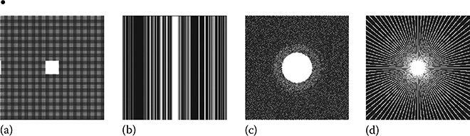
FIGURE 18.13
(a) Uniform sampling (26%), (b) random sampling (25%), (c) Gaussian sampling (20%), and (d) radial sampling (23%).

Periodic undersampling of k-space
Random omission of k-space lines in vertical direction
Gaussian random sampling of k-space
Radial sampling

Periodic undersampling is traditionally the most often used parallel MRI acceleration method. However, it is unsuitable for CS reconstruction. As we will see in the results section, it yields the worst results for CaLM MRI.

Randomly skipping k-space lines in the vertical direction has been used previously for CS-based MRI [18]. This gives better results than periodic undersampling.

Gaussian sampling yields extremely good results. In general, such sampling points cannot be efficiently acquired. However, when undersampling both phase-encoded directions in 3D scans, they can be efficiently acquired in two dimensions. Such sampling has been used in the past [52,53].

Radial sampling is by far the best suited practical and efficient sampling scheme for CS-based MR image reconstruction techniques. It is very fast and could be used for real-time MR data acquisition and is robust to object motion and ghosting artifacts.

There are four sets of ground-truth data used for our experimental evaluation (Figure 18.14). The brain data and the Shepp–Logan phantom have been used previously in [54]. The brain data come from a fully sampled T1-weighted scan of a healthy volunteer. The volunteer was scanned using spoiled gradient echo sequence with the following parameters—echo time = 8 ms, repetition time = 17.6 ms, and flip angle = 20°. The scan was performed by a GE Signa EXCITE 1.5 T scanner, using an eight-channel receiver coil. The eight-channel data for Shepp–Logan phantom were simulated. The UBC MRI Lab prepared a phantom by doping saline with Gd-DTPA. An MRI scanner with four-channel RF coil was used for acquiring the data using a FLASH sequence. In this work, we have selected slices one and seven for experimentation. The ground truth is formed by sum-of-squares reconstruction of the multichannel images.

Images

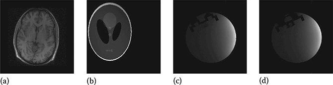
FIGURE 18.14
Ground-truth images: (a) brain, (b) Shepp–Logan phantom, (c) UBC MRI phantom slice 1, and (d) UBC MRI phantom slice 7.

We compare the proposed CaLM MRI with three state-of-the-art auto-calibrated methods—GRAPPA, l1SPIRiT, and CS SENSE. For non-Cartesian sampling, the GRAPPA operator gridding (GROG) method is used instead of GRAPPA. For CS SENSE and CaLM MRI, the mapping from non-Cartesian k-space to the Cartesian image space is the nonuniform fast Fourier transform (NUFFT).

For the CS SENSE and the proposed CaLM MRI, we tried orthogonal and redundant versions of Haar, Daubechies wavelets, and orthogonal fractional spline. But we found the best results were obtained for complex dual-tree wavelets. This has a small redundancy (factor of two) and has proved to yield good results on MR images in the past [22].

For CS SENSE, the sensitivity profiles are estimated in the fashion shown in [13]. A window at the center of the k-space is densely sampled, from which a low-resolution image for each coil is obtained. These images are combined by sum of squares. The sensitivity map is computed by dividing the low-resolution image of the corresponding coil by the combined sum-of-squares image.

The two objectives in this work are as follows:

To show that the reconstruction from existing parallel MRI techniques (CS SENSE, GRAPPA, and SPIRiT) is sensitive to the calibration stage. CaLM MRI however is not dependent on the calibration stage.
To show that our proposed CaLM MRI yields results that are at par with the best results obtained from state-of-the-art parallel MRI techniques—CS SENSE, GRAPPA, and SPIRiT.

For CS SENSE, the reconstruction accuracy is sensitive to the size of the calibration window, i.e., the size of the window used for densely sampling the center of the k-space. GRAPPA and SPIRiT are sensitive to the size of the calibration kernel and the calibration window. Here, the sizes of the calibration window and the calibration kernel are varied to show that the existing parallel MRI reconstruction methods are sensitive to the calibration stage.

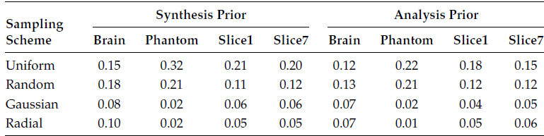
In the following, we first show the quantitative reconstruction results in Tables 18.7 through 18.10. The measure for reconstruction accuracy is the NMSE. Tables 18.7 through 18.9 show how the reconstruction accuracies from GRAPPA, l1SPIRiT, and CS SENSE are sensitive to their corresponding calibration stages. Table 18.10 tabulates results for CaLM MRI.

Tables 18.7 and 18.8 show the reconstruction results by the frequency domain methods—GRAPPA and l1SPIRiT. The results are plotted for three different calibration configurations and four different sampling schemes.

The first configuration is the default configuration as suggested in [54]. The calibration uses the maximum possible samples from the center of the k-space, and the kernel size is 5 × 5. The second configuration has a window size of 16 × 16 and a kernel size of 3 × 3, and the third configuration has a window size of 32 × 32 and a kernel size of 9 × 9. In the following tables, the configuration is written as window size and kernel size, i.e., 16, 3 denote a window size of 16 and kernel size of 3.

In Table 18.9, the reconstruction results from CS SENSE are tabulated. For CS SENSE, the sensitivity profile needs to be estimated/calibrated. In SENSE, the size of the calibration window determines the sensitivity map. Here, we show the results for three window sizes—16 × 16, 32 × 32, and 64 × 64.

TABLE 18.7
NMSE for GRAPPA Reconstruction

Images

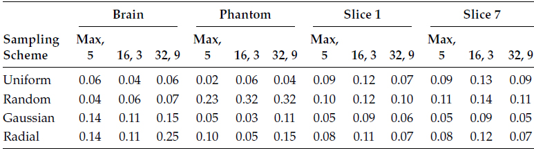
TABLE 18.8
NMSE for l1SPIRiT Reconstruction

Images

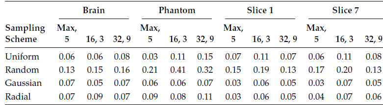
TABLE 18.9
NMSE for CS SENSE Reconstruction

Images

TABLE 18.10
NMSE for CaLM MRI Reconstruction

Images

For GRAPPA and l1SPIRiT, the average variation of reconstruction error is about 15% of the mean. For CS SENSE, the variation in reconstruction error is larger; it is about 25% of the mean. Moreover, there is not a single configuration that yields the best reconstruction results consistently.

Our proposed method CaLM MRI does not require any calibration. In the following table, the results from CaLM MRI method are shown. We show the results for both the synthesis and the analysis prior.

Even though we have shown the results for the analysis and the synthesis priors, we had already argued that the results from the analysis prior are expected to yield better results. This is in line with our previous work [22]. As mentioned before, CaLM MRI does not show good results for uniform undersampling. For the other Gaussian and radial sampling schemes, CaLM MRI method is at par with or even better than the best reconstruction results from GRAPPA, l1SPIRiT, and CS SENSE.

For visual qualitative evaluation, we provide the reconstructed brain images. Radial and Gaussian samplings show good results for all the reconstruction methods. For GRAPPA, l1SPIRiT, and CS SENSE, the images corresponding to the best configuration are shown. Since the UBC MRI slices are similar in nature and have very close reconstruction accuracies, we only show results for slice 1 during qualitative evaluation in Figures 18.15 and 18.16.

l1SPIRiT yields by far the best reconstruction results in terms of visual assessment. Both GRAPPA and CS SENSE show reconstruction artifacts. The reconstructed images are grainy (much like taking a picture with a digital camera in low light with high film speed). CaLM MRI (both analysis and synthesis prior) does not produce grainy reconstruction artifacts. For the synthetic Shepp–Logan phantom and the UBC MRI slices, our method is as good as l1SPIRiT. But for the anatomical image of the brain, CaLM MRI method produces a slightly smooth reconstruction.

The results from CaLM MRI are at par with the best results (at least for the data available with us) obtained from state-of-the-art multicoil parallel MR image reconstruction. The main advantage of our CaLM MRI method is that it does not require any calibration, unlike the other methods. This is a significant advantage since it is known that the parametric reconstruction methods are sensitive to the calibration stage.

Images

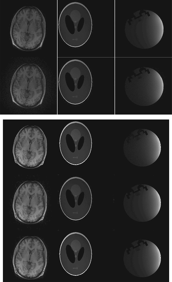
FIGURE 18.15
Reconstructed images from radial sampling. Left to right: brain, Shepp–Logan phantom, and UBC MRI slice 1; top to bottom: l1SPIRiT, GRAPPA, CS SENSE, CaLM MRI synthesis, and CaLM MRI analysis.

Images

FIGURE 18.16
Reconstructed images from Gaussian sampling. Left to right: brain, Shepp–Logan phantom, and UBC MRI slice 1; top to bottom: l1SPIRiT, GRAPPA, CS SENSE, CaLM MRI synthesis, and CaLM MRI analysis.

18.5 Conclusion

This chapter discusses some recent techniques in accelerating single-channel and multichannel MRI scans. Most of these techniques are based on the development of a newly developed branch of signal processing called CS. The main idea is to collect less k-space samples than is traditionally acquired and to use a smart reconstruction method to obtain good-quality images. CS-based techniques exploit the spatial redundancy of the images in order to reconstruct them from subsampled k-space measurements. The fundamentals of CS are briefly discussed in Section 18.2.

In Section 18.3.1, we discuss the problem of single-channel MRI reconstruction. There are different CS formulations that can be used for image recovery. The problem is that different researchers claim the superiority of their own method over others. This becomes a source of confusion to the practitioner who does not know which method to use. We review the different CS-based techniques that are used for MR image recovery and evaluate them via thorough experimentation. We find that the analysis prior formulation yields the best reconstruction results.

CS-based methods exploit the spatial redundancy of an MR image in terms of its transform domain sparsity. In Section 18.3.2, we showed that instead of exploiting the sparsity (in a transform domain), it is possible to recover the image by exploiting its rank deficiency. We showed that this technique yields the same reconstruction accuracy as CS-based methods but has about an order of magnitude faster reconstruction time.

Section 18.4 discusses the problem of multichannel parallel MRI reconstruction. In the parallel MRI problem, both the image and the sensitivity maps are unknown. However, joint solution of the two leads to an intractable problem. All parallel MRI reconstruction algorithms assume that the sensitivity maps either are provided or can be estimated from the data itself. Traditionally, the SENSE is an optimal method for parallel MRI reconstruction when the sensitivity maps are known. The sensitivity maps are either estimated from calibration scans or estimated from the actual data itself. Both of these estimation techniques are error prone, and the error introduced during the sensitivity map estimation unfortunately affects the final reconstructed image.

In Section 18.4.1, we discuss the variations of the basic SENSE technique. After the advent of CS, SENSE reconstruction is regularized by introducing sparsity promoting terms into the optimization problem. This, however, does not lead to any major improvement—the problem introduced from the sensitivity map estimation still remains. In recent studies, it has been shown how the SENSE reconstruction can be made robust against initial errors introduced during the sensitivity map estimation process. These methods iteratively reconstruct the maps and the MR image. They start with the initial estimates of the maps. Given the maps, they reconstruct the image. In the next iteration, they estimate the maps given the image. This procedure continues till convergence. There are two such studies—JSENSE and iSENSE. Both of them are more robust than the SENSE method. The iSENSE yields better reconstruction than the JSENSE.

The iSENSE and JSENSE though robust are not insensitive to the map estimation errors. In Section 18.4.2, we discuss our proposed CaLM MRI method. This technique does not require any explicit or implicit estimation of the sensitivity maps. It performs better than commercial and state-of-the-art techniques in MRI reconstruction.

References

1. D. Donoho, Compressed sensing, IEEE Transactions on Information Theory, 52(4), 1289–1306, 2006.

2. E. Candès, Compressive sampling, International Congress of Mathematicians, 3, 1433–1452, 2006.

3. E. Candès, J. Romberg, and T. Tao, Stable signal recovery from incomplete and inaccurate measurements, Communications on Pure and Applied Mathematics, 59(8), 1207–1223, 2006.

4. D. L. Donoho, For most large underdetermined systems of linear equations the minimal l1-norm solution is also the sparsest solution, Communications on Pure and Applied Mathematics, 59(6), 797–829, 2006.

5. J. Tropp and A. Gilbert, Signal recovery from random measurements via orthogonal matching pursuit, IEEE Transactions on Information Theory, 53(12), 4655–4666, 2007.

6. D. Needell and R. Vershynin, Uniform uncertainty principle and signal recovery via regularized orthogonal matching pursuit, Foundations of Computational Mathematics, 9(3), 317–334, 2009.

7. T. Blumensath and M. E. Davies, Stagewise weak gradient pursuits, IEEE Transactions on Signal Processing, 57(11), 4333–4346, 2009.

8. R. Saab, R. Chartrand, and Ö. Yilmaz, Stable sparse approximation via noncon-vex optimization, IEEE International Conference on Acoustics, Speech, and Signal Processing, Las Vegas, NV, pp. 3885–3888, 2008.

9. R. Saab and Ö. Yllmaz, Sparse recovery by non-convex optimization—Instance optimality, Applied and Computational Harmonic Analysis, 29(1), 30–48, 2010.

10. R. Chartrand and V. Staneva, Restricted isometry properties and nonconvex compressive sensing, Inverse Problems, 24(035020), 1–14, 2008.

11. R. Chartrand, Exact reconstruction of sparse signals via nonconvex minimization, IEEE Signal Processing Letters, 14, 707–710, 2007.

12. J. Trzasko and A. Manduca, Highly undersampled magnetic resonance image reconstruction via homotopic l0-minimization, IEEE Transactions on Medical Imaging, 28(1), 106–121, 2009.

13. K. T. Block, M. Uecker, and J. Frahm, Iterative image reconstruction using a total variation constraint, Magnetic Resonance in Medicine, 57(6), 1086–1098, 2007.

14. B. Liu, L. Ying, M. Steckner, J. Xie, and J. Sheng, Regularized sense reorthogonalization, using iteratively refined total variation method, IEEE International Symposium on Biomedical Imaging, Washington, DC, pp. 121–124, 2007.

15. S. Nam, M. E. Davies, M. Elad, and R. Gribonval, The co-sparse analysis model and algorithms, Applied and Computational Harmonic Analysis, 34(1), 30–56, 2013.

16. M. Elad, P. Milanfar, and R. Rubinstein, Analysis versus synthesis in signal priors, Inverse Problems, 23, 947–968, 2007.

17. M. Guerquin-Kern, D. Van De Ville1, C. Vonesch, J.-C. Baritaux, K. P. Pruessmann, and M. Unser, Wavelet-regularized reconstruction for rapid MRI, IEEE International Symposium on Biomedical Imaging, Boston, MA, pp. 193–196, 2009.

18. M. Lustig, D. L. Donoho, and J. M. Pauly, Sparse MRI: The application of compressed sensing for rapid MR imaging, Magnetic Resonance in Medicine, 58(6), 1182–1195, 2007.

19. S. Ma, W. Yin, Y. Zhang, and A. Chakraborty, An efficient algorithm for compressed MR imaging using total variation and wavelets, IEEE International Conference on Computer Vision and Pattern Recognition, Anchorage, AK, 2008.

20. R. Chartrand, Fast algorithms for nonconvex compressive sensing: MRI reconstruction from very few data, IEEE International Symposium on Biomedical Imaging, Boston, MA, pp. 262–265, 2009.

21. I. W. Selesnick and M. A. T. Figueiredo, Signal restoration with overcomplete wavelet transforms: Comparison of analysis and synthesis priors, Proceedings of SPIE, 7446 (Wavelets XIII), 2009.

22. A. Majumdar and R. K. Ward, Under-determined non-Cartesian MR reconstruction, Medical Image Computing and Computer Assisted Intervention, Beijing, China, pp. 513–520, 2010.

23. A. Majumdar and R. K. Ward, On the choice of compressed sensing priors: An experimental study, Signal Processing: Image Communication, 27(9), 1035–1048, 2012.

24. I. Baeza, J. A. Verdoy, R. J. Villanueva, and J. V. Oller, SVD lossy adaptive encoding of 3D digital images for ROI progressive transmission, Image and Vision Computing, 28(3), 449–457, 2010.

25. A. Al-Fayadh, A. J. Hussain, P. Lisboa, and D. Al-Jumeily, An adaptive hybrid image compression method and its application to medical images, IEEE International Symposium on Biomedical Imaging, Paris, France, pp. 237–240, 2008.

26. B. Recht, W. Xu, and B. Hassibi, Necessary and sufficient conditions for success of the nuclear norm heuristic for rank minimization, 47th IEEE Conference on Decision and Control 2008, Cancun, Mexico, pp. 3065–3070, 2008.

27. B. Recht, W. Xu, and B. Hassibi, Null space conditions and thresholds for rank minimization, Mathematical Programming, Cary, NC, 2010.

28. B. Recht, M. Fazel, and P. A. Parrilo, Guaranteed minimum rank solutions to linear matrix equations via nuclear norm minimization, SIAM Review, 52, 471–501, 2010.

29. K. Dvijotham and M. Fazel, A nullspace analysis of the nuclear norm heuristic for rank minimization, IEEE International Conference on Acoustics, Speech, and Signal Processing, Dallas, TX, March 2010.

30. A. Majumdar and R. K. Ward, An algorithm for sparse MRI reconstruction by Schatten p-norm minimization, Magnetic Resonance Imaging, 29(3), 408–417, 2011.

31. E. van den Berg and M. P. Friedlander, Probing the Pareto frontier for basis pursuit solutions, SIAM Journal on Scientific Computing, 31(2), 890–912, 2008.

32. R. M. Larsen, Lanczos bidiagonalization with partial reorthogonalization, Department of Computer Science, Aarhus University, Technical Report, DAIMI PB-357, September 1998. http://soi.stanford.edu/∼rmunk/PROPACK/

33. K. P. Pruessmann, M. Weiger, M. B. Scheidegger, and P. Boesiger, SENSE: Sensitivity encoding for fast MRI, Magnetic Resonance in Medicine, 42, 952–962, 1999.

34. D. K. Sodickson and W. J. Manning, Simultaneous acquisition of spatial harmonics (SMASH): Fast imaging with radiofrequency coil arrays, Magnetic Resonance in Medicine, 38(4), 591–603, 1997.

35. M. A. Griswold, P. M. Jakob, R. M. Heidemann, M. Nittka, V. Jellus, J. Wang, B. Kiefer, and A. Haase, Generalized autocalibrating partially parallel acquisitions (GRAPPA), Magnetic Resonance in Medicine, 47(6), 1202–1210, 2002.

36. M. Blaimer, F. Breuer, M. Mueller, R. M. Heidemann, M. A. Griswold, and P. M. Jakob, SMASH, SENSE, PILS, GRAPPA: How to choose the optimal method, Topics in Magnetic Resonance Imaging, 15(4), 223–236, 2004.

37. F. H. Lin, T. Y. Huang, N. K. Chen, F. N. Wang, S. M. Stufflebeam, J. W. Belliveau, L. L. Wald, and K. K. Kwong, Functional MRI using regularized parallel imaging acquisition, Magnetic Resonance in Medicine, 54(2), 343–353, 2005.

38. S. Ramani and J. A. Fessler, Parallel MR image reconstruction using augmented Lagrangian methods, IEEE Transactions on Medical Imaging, 30(3), 694–706, 2011.

39. B. Liu, K. King, M. Steckner, J. Xie, J. Sheng, and L. Ying, Regularized sensitivity encoding (SENSE) reconstruction using Bregman iterations, Magnetic Resonance in Medicine, 61, 145–152, 2009.

40. D. Liang, B. Liu, J. Wang, and L. Ying, Accelerating SENSE using compressed sensing, Magnetic Resonance in Medicine, 62(6), 1574–1584, 2009.

41. A. Majumdar and R. K. Ward, Nuclear norm regularized SENSE reconstruction, Magnetic Resonance Imaging, 30(2), 213–221, 2012.

42. L. Ying and J. Sheng, Joint image reconstruction and sensitivity estimation in SENSE (JSENSE), Magnetic Resonance in Medicine, 57, 1196–1202, 2007.

43. C. Fernández-Granda and J. Sénégas, L1-norm regularization of coil sensitivities in non-linear parallel imaging reconstruction, International Society for Magnetic Resonance in Medicine 2010, Stockholm, Sweden, 2010.

44. E. J. Candès and J. Romberg, Sparsity and incoherence in compressive sampling, Inverse Problems, 23(3), 969–985, 2007.

45. D. K. Sodickson and C. A. McKenzie, A generalized approach to parallel magnetic resonance imaging, Medical Physics, 28(8), 1629–1643, 2001.

46. R. G. Baraniuk, V. Cevher, M. F. Duarte, and C. Hegde, Model-based compressive sensing, arXiv:0808.35 72v5.

47. J. Huang and T. Zhang, The benefit of group sparsity, Annals of Statistics, 38(4), 1978–2004, 2010.

48. E. van den Berg and M. P. Friedlander, Theoretical and empirical results for recovery from multiple measurements, IEEE Transactions on Information Theory, 56(5), 2516–2527, 2010.

49. A. Majumdar and R. K. Ward, Non-convex group sparsity: Application to color imaging, IEEE International Conference on Acoustics, Speech, and Signal Processing, Dallas, TX, pp. 469–472, 2010.

50. A. Majumdar and R. K. Ward, Accelerating multi-echo T2 weighted MR imaging: Analysis prior group sparse optimization, Journal of Magnetic Resonance, 210(1), 90–97, 2011.

51. A. Majumdar and R. K. Ward, Compressive color imaging with group sparsity on analysis prior, IEEE International Conference on Image Processing, Hong Kong, China, pp. 1337–1340, 2010.

52. R. Chartrand, Nonconvex compressive sensing and re construction of gradient-sparse images: Random vs. tomographic Fourier sampling, IEEE International Conference on Image Processing (ICIP), San Diego, CA, 2008.

53. M. Lustig, D. L. Donoho, and J. M. Pauly, Rapid MR imaging with compressed sensing and randomly under-sampled 3DFT trajectories, Proceedings of the 14th Annual Meeting of ISMRM, Seattle, WA, 2006.

54. M. Lustig and J. M. Pauly, SPIRiT: Iterative self- consistent parallel imaging reconstruction from arbitrary k-space, Magnetic Resonance in Medicine, 64, 457–471, 2010.

55. A. Majumdar and R. K. Ward, Calibration-less multi-coil MR image reconstruction, Magnetic Resonance Imaging, 30(7), 1032–1045, 2012.

* W^TW = I = WW^T.

^†W^TW = I ≠ WW^T.

* The images, especially the difference images, should be viewed on a computer screen. The contrast resolution required for observing the fine variations is not fulfilled by most printers.

..................Content has been hidden....................

You can't read the all page of ebook, please click here login for view all page.

Table of Contents for
18 Multicoil Parallel MRI