22 Medical Image Registration: A Review

With the advent of different medical imaging modalities, clinicians can now perform diagnosis in a minimally invasive manner. Nevertheless, each modality currently only provides particular types of information. CT and MRI, for example, provide structural information of our body (e.g., an anatomical map), but do not convey functional information^* (i.e., relating to metabolic functions of an imaged organ). Conversely, modalities such as PET and SPECT capture functional but not structural information. This motivates image registration, the task of bringing two medical images into spatial alignment. Once images are aligned, information from different modalities can then be integrated and examined as a whole.

MIR indeed is a crucial step for many image analysis problems where information from different sources are combined and examined. The images involved may come from the same modality but captured at different times, or from multiple modalities and/or at different times, for example, as introduced earlier. Some general applications of MIR are listed in the following; more can be found in [18,38,89,160].

Multi-temporal image analysis. Images of the same subject are acquired at different times and/or under different physical conditions. Registration of these intra-subject images allows us to monitor disease progression, or to detect and/or quantify changes in an anatomy. Registration of intra-operative (between preoperative and postoperative) images can also enhance surgical procedures.
Multi-subject image analysis. Also known as (aka) intersubject registration; images of different subjects are registered for deformation-based morphology [8,114]. The subjects may also be of different species (e.g., human brain to chimpanzee brain for “asymmetry analysis” [7]).
Multimodality image fusion. As introduced earlier, images acquired from different modalities are aligned to create image fusions that facilitate clinical diagnosis [44,113]. Some clinical applications may also involve matching images of different dimensionality.
Construction and use of atlases. Group of images that are acquired from different sites and/or at different times are aligned simultaneously. This allows for statistical analysis of anatomical shapes [146], creation of probabilistic segmentations [139], brain functional localization [43], etc.
Dynamic image sequence analysis. This analysis involves dynamic stacking static images that were acquired at different time steps form dynamic image sequences, which are typically used to capture and quantify motion of an anatomy, for example, respiratory/cardiac cycle of the lungs/heart. One example application is the fusion of 2D+time ultrasound with 2D+time MRI to measure the distensibility of carotid arteries [87].

As we will see later, most of the proposed techniques for the aforementioned problems involve performing the following tasks: (1) characterizing the registration solution, which may involve a set of constraints imposed on the desired solution; (2) defining a list of criteria to quantify the optimality of a candidate solution; and (3) devising a strategy to find the desired solution. In the coming sections, we will individually examine the essential components central to each task. Let us first review the preliminaries to MIR.

22.2 Preliminaries

22.2.1 Image Representation and Imaging Terminologies

A digital image I gives a discrete representation of a continuous signal that measures physical quantities (e.g., light in photographs, or photon densities in an x-ray image). Following conventions of [56,92], the term physical or world coordinate is used to describe an arbitrary location in a continuous domain and the term image coordinate is used to index a particular cell on the image grid. We also refer to the data value at a grid center as its intensity value (“pixel” or “voxel” are also used in the context of a 2D or 3D domain, respectively) and denote a physical coordinate as x (in 2D, x = [x₁ x₂] represents the position of a point in the x and y dimensions).

Typically, structural images acquired from invisible light medical imaging modalities are scalar functions, that is, I: Ω ↦ ℝ^r, r = 1. For color images, or visible light medical images in general (e.g., dermoscopy, wound care imageries, etc.), I is a vector-valued function with r = 3. When I is an image sequence that is acquired to capture dynamic information occurring over time which is typically created by stacking static images to form 2D + time or 3D + time data, one may instead denote as I: ℝ^d × ℝ ↦ ℝ^r.

22.2.2 Data Interpolation

When one wants to query for intensity values at locations between cell centers (e.g., one third position of a cell), one must approximate these values from the original data. This is known as image interpolation or image resam-pling, and is usually done in a process where a continuous function is fitted to the original set of data points.

Common interpolation methods include nearest neighbor, linear (bi- or tri-), polynomial (cubic, quintic, etc.), and windowed sinc. Other less commonly used ones include Lagrange and Gaussian interpolation, as well as methods based on the Fourier and Wavelet transforms. For details on the latter methods proposed, see the survey of [72].

The simplest interpolation method is nearest neighbor (aka piecewise constant or proximal interpolation) where the intensity value of x is determined as the intensity value of its closest grid location. However, being a discontinuous function, nearest neighbor is not normally used for registration.

The more commonly used interpolant is linear interpolation (bilinear and trilinear for 2D and 3D, respectively). In 2D, it is defined as

\begin{matrix} ℐ_{l i n e a r} (x, I) = (1 - ε_{1}) (1 - ε_{2}) I (i_{1}, i_{2}) + ε_{1} (1 - ε_{2}) I (i_{1} + 1, i_{2}) \\ + (1 - ε_{1}) ε_{2} I (i_{1}, i_{2} + 1) + ε_{1} ε_{2} I (i_{1} + 1, i_{2} + 1) \end{matrix}

$\begin{matrix} ℐ_{l i n e a r} (x, I) = (1 - ε_{1}) (1 - ε_{2}) I (i_{1}, i_{2}) + ε_{1} (1 - ε_{2}) I (i_{1} + 1, i_{2}) \\ + (1 - ε_{1}) ε_{2} I (i_{1}, i_{2} + 1) + ε_{1} ε_{2} I (i_{1} + 1, i_{2} + 1) \end{matrix}$

Images

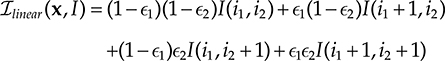
where i₁ and ∊₁ are, respectively, the integer and remainder parts of x₁ (similarly defined for those of x₂). Unlike nearest neighbor, it generates spatially continuous intensity values. However, it is not differentiable at the center of grid cells, which is a problem when a gradient-based optimization technique is used to optimize the registration objective (see Section 22.3.4.2). It also causes spatially varying, low-pass filtering of the images [38], which can be a problem when computing similarity metrics on image pairs.

From the perspective of signal processing theory, the most ideal interpo-lant is one that uses the sine function because it has the fullest potential to recover the continuous signal underlying I [56,72]. For reasons of practicality, the sine function is only approximated with a Window function w. In 2D, a windowed sine interpolant is defined as

ℐ_{s i n c} (x, I) = \sum_{p = ⌊ x_{1} ⌋ + 1 - m}^{⌊ x_{1} ⌋ + m} \sum_{q = ⌊ x_{2} ⌋ + 1 - m}^{⌊ x_{2} ⌋ + m} I (x) K (x_{1} - p) K (x_{2} - q), (22.1)

$ℐ_{s i n c} (x, I) = \sum_{p = ⌊ x_{1} ⌋ + 1 - m}^{⌊ x_{1} ⌋ + m} \sum_{q = ⌊ x_{2} ⌋ + 1 - m}^{⌊ x_{2} ⌋ + m} I (x) K (x_{1} - p) K (x_{2} - q), (22.1)$

where m is the radius or spatial extent of w and

K (t) = w (t) \sin c (t) (22.2)

$K (t) = w (t) \sin c (t) (22.2)$

Nevertheless, the windowed sine interpolant has several trade-offs in its utilization, for example, large m, while being more precise, will require longer computation times [144].

Spline interpolation may arguably give optimal balance between computation time and precision of interpolation [73]. The spline interpolant involves representing the continuous form of I by a set of spline basis functions β_j and computing a set of expansion coefficients c_j of β_j such that the resulting basis function interpolates the values of I at grid locations. The set of coefficients are computed by solving a linear system of equations, which is most effi-ciently done by recursive digital filtering. Intensity at x is computed by multiplying the B-spline coefficients with shifted B-spline kernels within a small support region of the requested position; in 2D, this is done as

ℐ_{s p l i n e} (x, I) = \sum_{j} c_{j} β^{(d)} (x - x_{j}) (22.3)

$ℐ_{s p l i n e} (x, I) = \sum_{j} c_{j} β^{(d)} (x - x_{j}) (22.3)$

where j indices the pixel coordinates within the support region of the spline window.

22.2.3 Spatial (Geometric) Transformations

In image registration, a spatial transform plays the crucial role of representing registration solutions in a precise manner. Mathematically, it may be defined as U: Ω ↦ ℝ^d, Ω ⊆ ℝ^d, which describes a mapping between the coordinate system of one image and that of another image.

22.2.3.1 Terminologies

A mapping U is said to be smooth if all of its partial derivatives of up to a certain order exist and are continuous. It is said to be bijective if it is a one-to-one mapping. It is said to be invertible (aka homeomorphic or topology-preserving) if it is bijective and continuous, and that its inverse is also continuous. Note that smoothness of U is not equivalent to invertibility, that is, invertibility does not require differentiability of U. When U is both smooth and invertible, it is called diffeomorphic.

Some of these properties of U are highly desirable; after all, properties of U affect the appearance of the image to which it is applied. Generally, smoothness of U is desired as it directly affects the smoothness of the image on which it is applied to. Applying a random warp (vector field with random displacements) to an image, for instance, will destroy the morphology (level sets) of an image [34].

Bijectivity, on the other hand, may or may not be required. Bijectivity of U ensures that the folding of space does not happen as multiple points cannot be mapped into the same point. In some cases, however, the folding of space should be allowed. This occurs, for example, in intra-operative image registration where tearing and resection of tissues can occur in the postoperative image. Even for registration of intersubject brain images, the topology of the brain, the shape of the ventricles, the number and shape of the sulci may vary significantly from one subject to another [114] such that bijectivity should not be strictly enforced.

Invertibility also may or may not be required. It is needed when one needs to map individual images from a set to a common space. It is also needed in order to allow for decomposition of the transformation Jacobian, which is often done in registrations of diffusion tensor images to reorient tensor values at each location after deforming an image.

Lastly, we desire a diffeomorphic transform when we need to maintain the (non-) connectivities between neighboring anatomical structures after registration [12]. Note that a diffeomorphic transform that matches arbitrary number of points can always be found (proof given in [63]).

22.2.3.2 Spatial Transformation Models

Spatial transformation models (transforms) are often used to parameterize U, thereby allowing U to be compactly represented. The ones commonly used for image registration are categorized as either linear or nonlinear.

Linear transforms include translation, rotation, rigid, affine, and perspective. A rigid transform allows for translations and rotations only; an affine transform allows for rigid as well as scale and skew (distortions that preserve parallelism of lines); a projective transform allows for all distortions that preserve colinearity (lines remain straight after distortion).

Compared to linear models, nonlinear transformation models allow for more localized deformations. Common nonlinear models include those that are based on radial basis functions (RBF). Under these models, a set of points ℘ = {x_i}, for example, manually identified landmarks in Ω, is used to extrapolate U:

U (x) = H_{m - 1} (x) + \sum_{i} c_{j} β (x - P_{i}) . (22.4)

$U (x) = H_{m - 1} (x) + \sum_{i} c_{j} β (x - P_{i}) . (22.4)$

where

H_m₋₁ (x) is a polynomial of degree m − 1

β is a basis function

c_i are coefficients to be solved in a system of equations

Note that ℘ may be irregularly located in Ω. Different forms of β(r) results in different types of spline [124]. For example, with r = ‖x − ℘_i‖, defining the RBF as β(r) = r² ln r and β(r) = r gives the thin-plate-spline (TPS) in 2D and 3D, respectively. With (r² + a²), where 0 < b < 1 and a is a user-parameter that increases the amount of smoothing, one gets the multi-quadric splines (MQ). Other choices are described in [52,124].

Many RBFs like TPS and MQ give global support, that is, one control point has a global effect on U (i.e., deformations in one image region affects the entire domain). This property may cause problems as large and inconsistent displacements in ℘ can lead to singularities in the systems of equation to be solved. Furthermore, the size of ℘ directly affects computational complexity of solving the system.^* In these regards, basis functions with local support are highly desired.

One of such locally supported functions is the basis-spline (B-spline). When extended to a multivariate function via the use of tensor products, it gives the free-form deformation (FFD) model. Under FFDs, the image domain is divided into a lattice whose intersections represent the positions of a set of control points B such that translating the control points induces local deformations. Performing registration is then reduced to finding the optimal translations for each control point [46], or the optimal values of the set of B-spline coefficients [107], or the divergence^{^†} and curl of U at control point [54]. The DOFs of FFD is thus determined by the size of this set of parameters. The spacing between control points determines the scale of local deformations, for example, lowering the spacing allows for more localized motion. In 2D, it has the form:

U (x) = \sum_{l = 0}^{n} \sum_{m = 0}^{n} β_{l, n} (r) β_{m, n} (s) B_{i + l, j, m} . (22.5)

$U (x) = \sum_{l = 0}^{n} \sum_{m = 0}^{n} β_{l, n} (r) β_{m, n} (s) B_{i + l, j, m} . (22.5)$

where

β.,. is a basis function of degree n

(r, s) are lattice coordinates relative to x

Despite some of its deficiencies [126], FFD is a popular choice in many applications due to its ease of implementation, low computational complexity, and the superior properties of B-spline functions (continuity and locality).

Another popular choice is to represent U with finite elements [102,122], which involves discretizing Ω with mesh elements, each with a set of meshes. To obtain values of U at points within a mesh element e, one then uses linear interpolation:

U (x) = \sum_{l = 0}^{n} B^{2} (q_{l}^{e}) {[U (q_{1}^{e}) U (q_{1}^{e}) \dots U (q_{n}^{e})]}^{T} . (22.6)

$U (x) = \sum_{l = 0}^{n} B^{2} (q_{l}^{e}) {[U (q_{1}^{e}) U (q_{1}^{e}) \dots U (q_{n}^{e})]}^{T} . (22.6)$

where

B^e is a basis function for e

$q_{n}^{e}$ $q_{n}^{e}$ the nth node of mesh e

Lastly, parameterization of U has also been done with discrete Fourier transformation (DFT) [27] and discrete cosine transformation (DCT) [52], which involve globally supported basis functions (as they operate in frequency domain). Usually, only low-frequency basis functions are used for parameterization, which by construction gives inherently smooth regu-larized solutions [159]. Gefen [42] also modeled U with wavelet expansion and showed that its use can give more accurate registrations than use of TPS. However, the complexity of the wavelet approach depends on the size of U.

In summary, linear models and nonlinear models differ in terms of their DOFs, which in turn determine the different types of geometric distortions they induce on images. In some applications, linear models are sufficient to describe misalignment between two images, for example, registration of brain images. In others, both linear and nonlinear models are needed to correct for global and local misalignment between two images. There are also cases where misalignment between two images involve both articulation (e.g., of rigid bones) and elastic deformations (e.g., soft tissues surrounding rigid bones) such that the use of a global nonlinear transform will give elastic deformations everywhere, or conversely, the use of a global linear transform will fail to align elastic tissues. In these cases, a common strategy is to partition the image domain into different regions, determine a local (non) linear transform for each region, and employ a scheme to spatially fuse the piecewise local transforms [100]. Another approach is the use of polyrigid models [3]. Details on the aforementioned linear and nonlinear models can also be found in focused reviews [52,144] or general surveys [18,44,77,83].

22.3 Fundamentals of Image Registration

22.3.1 Mathematical Formulation of Image Registration

Let there be two images F and M. The goal of registering F and M is to find a spatial transformation U that optimally maps points in F to the corresponding points in M.^* Optimality of U is measured by a set of criteria of two types: regularization (aka internal forces), which measures the regularity of U, and data dissimilarity (aka external forces), which measures how well U relate F and M based on image data. Details on these terms will be surveyed in the following subsections. Once a set of criteria has been defined for a specific registration problem, the optimal U can then be found via minimization of a cost function C that contains a weighted sum of two or more of these criteria, for example,

C (U) = α_{i} D_{i} (F, M \circ U) + α_{i + 1} ℛ_{i + 1} (U) + \dots (22.7)

$C (U) = α_{i} D_{i} (F, M \circ U) + α_{i + 1} ℛ_{i + 1} (U) + \dots (22.7)$

where

$D_{i}$ $D_{i}$ denotes a data dissimilarity term

ℛ_i+1 denotes a regularization term

α_i is a weight on the ith term

22.3.2 Regularization

Solution of an image registration problem, U, is generally not unique.^{^†} To reg-ularize U, we may restrict the type of U to a certain space, such as the space of affine transformations or the space of diffeomorphisms (Section 22.4.1). We may also explicitly enforce constraints on the behavior of U based on our prior knowledge about the expected solution. For example, when registering x-ray breast images, one might impose incompressibility constraints in tissue deformation [104]. When registering images containing rigid bodies (e.g., bones [129]) one might impose local rigidity constraints to disallow elastic deformations in rigid regions.

In Section 22.2.3, we have outlined the desired properties of U, including smoothness and invertibility, arguably two of the most important ones. We next present how these may be achieved. Other regularization constraints proposed in the literature are highlighted in Section 22.3.2.4.

22.3.2.1 Smoothness Regularization: Implicit Approaches

A common approach to regularization is to constrain the behavior of U via use of a spatial transformation model. As discussed previously, these models impose constraints on the type of geometric distortions they induce on images. For example, rigid transforms preserve all internal angles and distances, perspective transforms only preserve colinearity (points that lie on a line remain so after they have undergone transformation), while nonlinear transforms allow for localized deformations.

Solving U using parametric transforms generally simplifies the optimization of the objective function (Equation 1.7). Rather than solving for U at each spatial location in Ω (c.f. Section 22.4.1), one only needs to resolve the transform's parameters, effectively reducing the size of the solution space (in case of linear transforms, the dimension of the search space is equal to the number of transform parameters). Furthermore, the inherent smoothness properties provided by a given spatial transformation model ensure some regularity of U. Thus, in many older works, for example [82], no explicit regularization was done. However, in more recent works, invertibility has become an important criterion [29]. As all of the aforementioned parametric models do not enforce invertibility, additional regularization terms are needed; these will be examined in Section 22.3.2.4.1.

22.3.2.2 Smoothness Regularization: Explicit Approaches

When no parameterization of U is used, any point may be displaced arbitrarily, which would lead to an unrealistic warp of M. To ensure smoothness of U, as well as other desired properties of U outlined in Section 22.2.3, explicit energy terms are needed (ℛ_i+1 in Equation 22.7). We now examine in detail some of the common ones found in the literature.

22.3.2.2.1 Regularizers Motivated from Basis Functions

Regularization terms in Equation 22.7 are typically defined based on an application-dependent Sobolev semi-norm (bilinear form) [90]:

ℛ_{n o r m} (U) = {‖ L (U) ‖}_{L_{2} {(Ω)}^{q}} d x (22.8)

$ℛ_{n o r m} (U) = {‖ L (U) ‖}_{L_{2} {(Ω)}^{q}} d x (22.8)$

where L is a differential operator on U.

One regularizer proposed by Horn and Schunk [53] is the diffusion regularizer, which penalizes variations in the gradients of U. In 2D, it is defined as

ℛ_{d i f f} (U) = \frac{1}{2} \int_{x \in Ω} \sum_{i}^{d} {‖ \nabla U_{i} (x) ‖}^{2} d x (22.9)

$ℛ_{d i f f} (U) = \frac{1}{2} \int_{x \in Ω} \sum_{i}^{d} {‖ \nabla U_{i} (x) ‖}^{2} d x (22.9)$

where U_i(x) denotes the ith component of U at x. This definition relates closely to the classical Tikhonov regularization for ill-posed problems. When instead an L¹ norm is used, such regularization falls in the class of total variation (TV) methods [10,41], leading to a TV regularizer that is defined as

ℛ_{T V} (U) = \int_{x \in Ω} \sum_{i}^{d} | \nabla U_{i} (x) | d x (22.10)

$ℛ_{T V} (U) = \int_{x \in Ω} \sum_{i}^{d} | \nabla U_{i} (x) | d x (22.10)$

which allows for discontinuities in U. However, as it is non-differentiable at zero, researchers have proposed to replace |x| with $\sqrt{x^{2} + k^{2}}$ $\sqrt{x^{2} + k^{2}}$ where value of k affects amount of discontinuities allowed.

Note that the aforementioned regularizers also penalize linear transformations [92]. To address this, the curvature regularization (aka bi-harmonic) [20,92] was proposed:

ℛ_{c u r v} (U) = \frac{1}{2} \int_{x \in Ω} \sum_{i}^{d} Δ U_{i} {(x)}^{2} d x (22.11)

$ℛ_{c u r v} (U) = \frac{1}{2} \int_{x \in Ω} \sum_{i}^{d} Δ U_{i} {(x)}^{2} d x (22.11)$

which approximates the mean curvature of the surface of U. By taking the Laplacian of U instead of its gradient, linear transforms result in zero smoothness cost. Furthermore, as the null-space of the operator has infinite dimension and contains all harmonic vector fields, use of this regularizer ensures smooth deformations [92].

Another common regularizer is based on the thin-plate-spline model (Section 22.2.3):

ℛ_{t h i n - p l a t e} (U) = \frac{1}{2} \int_{x \in Ω} (\frac{\partial^{2} U (x)}{\partial^{2} x_{1}} + 2 \frac{\partial^{2} U (x)}{\partial x_{1} \partial x_{2}} + \frac{\partial^{2} U (x)}{\partial^{2} x_{2}}) d x . (22.12)

$ℛ_{t h i n - p l a t e} (U) = \frac{1}{2} \int_{x \in Ω} (\frac{\partial^{2} U (x)}{\partial^{2} x_{1}} + 2 \frac{\partial^{2} U (x)}{\partial x_{1} \partial x_{2}} + \frac{\partial^{2} U (x)}{\partial^{2} x_{2}}) d x . (22.12)$

Note that this regularization term is zero for any affine transformations and therefore penalizes only non-affine transformations.

In [22], Chen and Suter proposed a generalization of the scalar thin-plate splines (TPS) called the m-order regularization:

ℛ_{d i v + c u r l} (U) = \frac{1}{2} \int_{Ω} β_{1} {| \nabla^{m} d i v U |}^{2} + β_{2} {| \nabla^{m} c u r l U |}^{2} d x (22.13)

$ℛ_{d i v + c u r l} (U) = \frac{1}{2} \int_{Ω} β_{1} {| \nabla^{m} d i v U |}^{2} + β_{2} {| \nabla^{m} c u r l U |}^{2} d x (22.13)$

where the divergence and curl operators are used to impose incompressible flow and irrotational flow, respectively, and β₁ and β₂ weight the respective components. According to [22], this regularizer is applicable in tagged cardiac MRI registration that require the solenoidal component of U to be divergence-free.

22.3.2.2.2 Regularizers Based on Continuum Mechanics

The linear-elastic and fluid-flow models are two classic physics-based regularization methods [52,92,103].^* Both models borrow concepts from continuum mechanics to describe the amount and type of forces exerted on a medium and model image deformations as responses to forces acting on either a elastic body or viscous fluid.

Elastic regularization is based on the theory of linear elasticity, which states that the body forces and “surface stresses” of a linear elastic material sum to zero when the material is in equilibrium, thus giving rise to the following Navier-Cauchy linear elastic partial differential equation (PDE) [52]:

μ \nabla^{2} U (x) + (μ + λ) \nabla {(\nabla \cdot U)}^{2} + f (x) = 0 (22.14)

$μ \nabla^{2} U (x) + (μ + λ) \nabla {(\nabla \cdot U)}^{2} + f (x) = 0 (22.14)$

where f denotes the body force; μ and λ are the Lame parameters, which can be interpreted in terms of Young's modulus and Poisson's ratio^{^†}, and are used to describe the relationship between stress and strain (internal forces that bring the material into equilibrium). The first term is associated to the incom-pressibility of the material [15,52]. The second term allows for expansion (dilation) or contraction of the material [17,124]. Formulating MIR with this PDE, f is modeled as matching forces based on image similarity (more details in Section 22.3.3) and the remaining terms are seen as internal forces that regu-larize U. Accordingly, elastic regularization can be formulated as [92]

ℛ_{e l a s t i c} (U) = \frac{1}{2} \int_{Ω} μ \nabla^{2} U (x) + (μ + λ) \nabla {(\nabla \cdot U)}^{2} d x . (22.15)

$ℛ_{e l a s t i c} (U) = \frac{1}{2} \int_{Ω} μ \nabla^{2} U (x) + (μ + λ) \nabla {(\nabla \cdot U)}^{2} d x . (22.15)$

The derivation of Equation 22.14 assumes that the stress and strain are linearly related, thus assuming that the elastic properties of the material is homogeneously by isotropic [52]. This is generally not true in many biological materials. In practical terms, the linear relationship assumes that the restoring forces increase monotonically with strain [29], thus penalizing large deformations. Additionally, ignoring the second-order derivatives of U would lead to large numerical errors for large deformations [52].

To address these problems, Christensen et al. [29] proposed a viscous-fluid-based model, which views a deforming image as a highly viscous (sticky and thick) fluid. Specifically, this model is built on several physical laws that govern conservation of mass, energy, linear and angular momentum. We will highlight two of the most relevant. The first is the constitutive equations [52], which state that the stress tensor Σstress is linearly related to the rate of deformation tensor D as follows:

Σ_{s t r e s s} = - p I + λ_{f} trace (D) I + 2 μ_{f} D (22.16)

$Σ_{s t r e s s} = - p I + λ_{f} trace (D) I + 2 μ_{f} D (22.16)$

where D is expressed as

D = \frac{1}{2} (\nabla V + {(\nabla V)}^{T}) (22.17)

$D = \frac{1}{2} (\nabla V + {(\nabla V)}^{T}) (22.17)$

with V being the instantaneous velocity of U.

The second is the conservation of linear momentum, which states that

\nabla ρ + f = ρ \frac{\partial V}{\partial t} + η V (22.18)

$\nabla ρ + f = ρ \frac{\partial V}{\partial t} + η V (22.18)$

where η is a parameter that allows for “arbitrary creation or destruction of mass.” Combining Equations 22.16 through 22.18 results in the Navier–Stokes–Duhem equation:

ρ \frac{\partial V}{\partial t} = f - \nabla p + μ_{f} \nabla^{2} U (x) + (μ_{f} + λ_{f}) \nabla {(\nabla \cdot V)}^{2} - η V (22.19)

$ρ \frac{\partial V}{\partial t} = f - \nabla p + μ_{f} \nabla^{2} U (x) + (μ_{f} + λ_{f}) \nabla {(\nabla \cdot V)}^{2} - η V (22.19)$

and assuming negligible change in ρ and ignoring^* the inertial terms $ρ \frac{\partial V}{\partial t}$ $ρ \frac{\partial V}{\partial t}$ and ηV) yield the following Navier–Stokes PDE:

V \nabla^{2} V (x) + (μ + λ) \nabla {(\nabla \cdot V)}^{2} + f (x) = 0 (22.20)

$V \nabla^{2} V (x) + (μ + λ) \nabla {(\nabla \cdot V)}^{2} + f (x) = 0 (22.20)$

Remarkably, Equation 22.20 is similar to Equation 22.14 except that this PDE operates on V instead of U. Intuitively, operating on V gives a more accurate calculation of the displacement gradients (second-order gradients of U are not ignored) leading to a more realistic model of material deformations.

22.3.2.3 Constraints for Invertibility

None of the aforementioned regularization methods detailed so far ensures invertibility of U. A simple approach to ensure invertibility is to add a regu-larization term to the registration objective function (Equation 22.7) that penalizes cases when |D| < 0.3 [106,126].

R_{in v e r t i b i l i t y} (U) = | D (x) - 1 | . (22.21)

$R_{in v e r t i b i l i t y} (U) = | D (x) - 1 | . (22.21)$

In [62], Chen and Lee showed that FFD based on cubic B-splines is locally injective over Ω if the maximum displacement of control points is limited to 0.40δ, where δ is the spacing of control point grid. This means that invert-ibility of U can also be ensured by constraining the maximum displacement of control points of an FFD lattice (e.g., control points on a lattice with 20 mm spacing should be constrained to translate no more than 8 mm). However, this restriction becomes impractical when one needs to recover large deformations (i.e., >8 mm). A better alternative may be the polyrigid/polyaffine transformation models proposed in [3].

22.3.2.4 Other Regularization Constraints

22.3.2.4.1 Inverse Consistency

Related to the invertibility constraint is inverse consistency, which demands that registration results be consistent or symmetric: if U₂ is the inverse transform of U, that is, M ° U = F and F ° U₂ = M, then U₂ ° U = Id [8,27]. Inverse consistency is important when the end-goal of MIR is to transfer some quan-titation from one image to another (e.g., segmentation via registration) such that results are invariant to choice of the reference image.

Theoretically, the process of finding an invertible transform is inherently symmetric; however, this is practically not true if an asymmetric data similarity cost is used [11]. One solution is to symmetrize the data term as done in [5,11,111], or to add a regularization that penalizes the residue between U and its inverse [26], for example,

ℛ_{in v - c o n s i s i s t e n c y} \sum_{x \in Ω} {‖ U^{- 1} (x) - U (x) ‖}^{2} . (22.22)

$ℛ_{in v - c o n s i s i s t e n c y} \sum_{x \in Ω} {‖ U^{- 1} (x) - U (x) ‖}^{2} . (22.22)$

22.3.2.4.2 Volume-Preservation

One may require U to be volume-preserving (VP), which is desired^* when F and M are known to be capturing the same anatomy that does not change in size. An interesting formulation of VP is based on the optimal mass transport problem of Monge-Kantorovich [127]. A simpler alternative is the incom-pressibility constraint:

ℛ_{j} (U) \int_{Ω} | \log (D (x)) | d x . (22.23)

$ℛ_{j} (U) \int_{Ω} | \log (D (x)) | d x . (22.23)$

Other forms include $\int_{Ω} | D (x) - 1 | d x$ $\int_{Ω} | D (x) - 1 | d x$ and those given in [104].

22.3.2.4.3 Local Rigidity

When registering images containing rigid objects (e.g., bones, hard tissues), one demands that these hard objects remain rigid after registration. One can do this by enforcing additional local rigidity constraints over selected regions; for example, in 2D [91]:

ℛ_{r i g i d i t y} (U) = \sum_{}^{} (\sum_{}^{} {‖ \frac{\partial^{2} U (x)}{\partial x_{i} \partial x_{j}} ‖}^{2} + {‖ J^{T} (x) J (x) - I d ‖}^{2} + {‖ D (x) - 1 ‖}^{2}) (22.24)

$ℛ_{r i g i d i t y} (U) = \sum_{}^{} (\sum_{}^{} {‖ \frac{\partial^{2} U (x)}{\partial x_{i} \partial x_{j}} ‖}^{2} + {‖ J^{T} (x) J (x) - I d ‖}^{2} + {‖ D (x) - 1 ‖}^{2}) (22.24)$

where each aforementioned term measures local deviations from area-preservation (linearity), angle-preservation (orthogonality), and VP, respectively. Another [48] formulates local rigidity as hard constraints. Pennec et al. [98] also measured local rigidity with trace((J^T J − Id)²).

22.3.3 Data (Dis)Similarity

The sources of information that the data (dis)similarity term is built upon can generally be classified as model-based or intensity-based [2,92].

Model-based information is often provided in forms of landmark correspondences identified by clinical experts or manual segmentation of the input images. Examples include [30] where Chui et al. used the Robust Point Matching algorithm to match manually extracted sulcal points for brain image registration, and [25,63] where researchers have matched landmarks via dif-feomorphic warps. Fuzzy or hard segmentation labels, too, can be matched using the cardinality match or Kappa statistics similarity metrics [56].

Due to the need for human intervention, accuracy of model-driven registration highly depends on the correctness of landmark correspondences or segmentation. When employing landmark correspondences, the identified landmarks should be spatially distributed [56,92]. When using segmentation, one needs to ensure that interpolation artifacts would not corrupt evaluations of image similarity. Consequently, pure use of model-based data terms is quite restrictive.

In contrast to model-based information, intensity-based information is derived entirely from the input images. This information may be based on raw image intensities or features extracted from the intensities.

In mono-modality registration, data similarity terms using information about raw intensities usually assume that the similarity between F and M is related to their intensity distributions. Assuming both F and M contain the same anatomy and U represents an optimal alignment, their intensity relationship becomes:

F = M \circ U + τ + ζ (22.25)

$F = M \circ U + τ + ζ (22.25)$

where

τ is zero-mean Gaussian noise

ζ is an intensity correction field

Essentially, Equation 22.25 states that after applying U to M, M and F only differ by an intensity mapping with an additive noise.

For some applications, e.g., CT-CT intra-subject image registrations, we may assume ζ = 0, thus allowing for the use of the Sum of Squared Difference (SSD) metric. If instead, intensities of F and M are linearly related, then one may use the (normalized) cross-correlation (CC) metric [5,144], the coefficient of variation [143], or those based on the normalized intensity gradients [49].

The assumption that ζ is zero or linear can easily be violated when images are corrupted by spatially-varying or “nonstationary” intensity distortions, for example, MR images. Real-world images are also often corrupted by spatially varying distortions, occlusions, illumination inhomogeneity, and reflectance artifacts [77,95].

To address intensity inhomogeneities, measures based on information theory may be used. These include joint entropy [92], entropy correlation coefficient [40], cumulative residual entropy [138], normalized mutual information (NMI) [2] and its numerous other extensions, for example, regional MI, alpha-MI, generalized survival exponential entropy–based MI (GSEE-MI) [75,78,81,107,137]. As these measures belong to a subclass of the divergence measures, which measures distances between distributions [101], they can be more robust against intensity inhomogeneities. However, while they are shown to be effective for many multimodal registration problems [2], these measures still assume global spatial dependencies between corresponding pixels. To better capture nonstationary dependencies, authors have proposed to compute these measures locally, that is, average over a small pixel neighborhood, based on the observation that spatially varying intensity distortion is constant within a small pixel neighborhood. Examples include local CC and regional MI.^* More explicit ways include performing intensity correction and registration simultaneously or removing ζ (via some training procedures, etc.) before metric evaluation [37,93,95]. Alternatively, Droske and Rumpf [34] proposed to match image level sets using a Mumford-Shah formulation for registration.

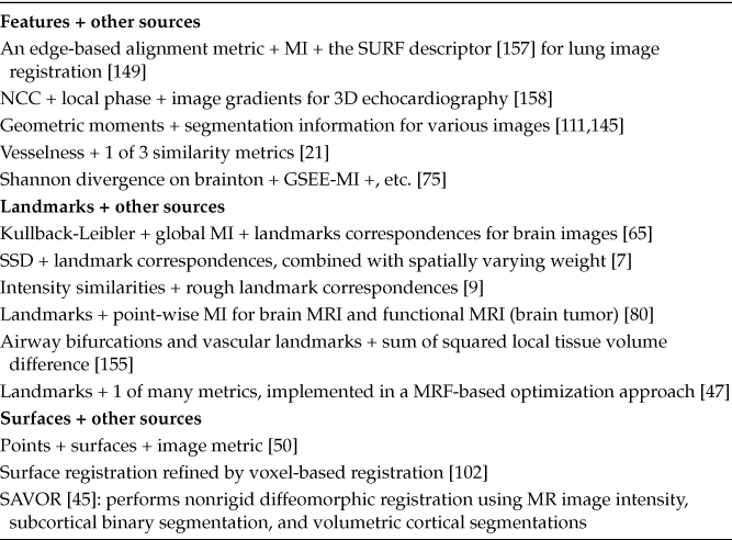
Data dissimilarity terms built on feature-based information generally involve extracting and using particular type of information from the images for registration. Edge-based features include edgeness, ridges, local curvature extrema, corners, crest, and extremal lines [17,83,96,149]. Others that examine the texture of image regions include Gabor [16] and grey level cooccurrence matrix (GLCM) [16], “braintons” [75], and Laws’ texture coefficients [60]. Features that analyze and capture the structural properties in images include vesselness [21], local structure [116], and moment invariants [39,151]. Those adopted from the computer vision community include SIFT [23], SURF [157], and shape context [1,128].

In the past decade, researchers began to adopt a hybrid approach where multiple sources of information are combined to improve existing metrics. One of the most prominent examples includes the HAMMER algorithm (Section 22.4.2), which combines segmentation-based information and geometric moment invariants (GMI), which are calculated in neighborhoods of different sizes. Avants et al. also [6] proposed the idea of integrating different image metrics and sources for DTI-registration (e.g., combining a correlation-based metric on T1 and FA images). Their software, too, allows users to combine multiple image metrics as well as landmarks. Hartkens et al. [50] also combined user-provided surface information with NMI for nonrigid registration of brain images, while Cao et al. [21] combined a feature-based measure with a conventional intensity-based measure for lung image registration. Table 22.1 highlights various other hybrid approaches.

22.3.4 Solution-Search

If the registration objective contains only one data term (e.g., Equation 22.7 contains D only), it may be possible to perform registration analytically, as we shall see in the next section. However, as Section 22.3.2 explained, reg-ularization constraints are generally needed, meaning that Equation 22.7 involves more than one energy term. Optimization methods are therefore needed to minimize a potentially complex and nonlinear objective function. Section 22.3.4.2 will highlight some of the optimization methods that have been devised for MIR.

22.3.4.1 Closed-Form Solutions for Image Registration

Most closed-form solutions for image registration operate on ordered point sets (point sets with known correspondences) that have been extracted from the images to be registered. As discussed in Section 22.2.3.2, if point correspondences are available, one may compute a nonlinear transform directly via TPS interpolation. It is also possible to resolve the parameters of a rigid transform between two ordered point sets in closed form. According to [36], the earliest method for closed-form rigid registration is based on minimization of a least squares (LS) error^* (known as fiducial registration error if the point correspondences originate from fiducial markers or expert-identified landmarks) and is solved via SVD. Its later variants include different formulations of the Eigen system describing the point correspondences. Three of such are described in [36].

TABLE 22.1
Hybrid Approaches to Construction of Data Dissimilarity Terms

Images

For affine motions based on least squares, regularization is needed to prevent all points in one point set to be mapped to a single point of the other set (as this would give an LS error of zero) [35]. For this, one may employ the Laplacian operator (i.e., L = a∇² + cI where a, b are constants) for regularization and allow for inexact point correspondences by assuming Gaussian distributed noise around each. This led to the following Bayesian energy minimization as proposed in [28]:

\arg \min_{U, A, t} \sum_{i = 1}^{m} [(A {P^{'}}_{i} + t) - (P_{i} - U (P_{i}))] σ_{i} [(A {P^{'}}_{i} + t) - (P_{i} - U (P_{i}))] + {‖ L U ‖}^{2} . (22.26)

$\arg \min_{U, A, t} \sum_{i = 1}^{m} [(A {P^{'}}_{i} + t) - (P_{i} - U (P_{i}))] σ_{i} [(A {P^{'}}_{i} + t) - (P_{i} - U (P_{i}))] + {‖ L U ‖}^{2} . (22.26)$

where

m is the number of correspondences

A, t are respectively the affine matrix and translation vector to be estimated

σ_i is the covariance matrix that represents the spatial uncertainty of the ith pair of correspondence

By inverting the system matrix of the following system of linear equations

\begin{matrix} (A {P^{'}}_{i} + t) = P_{i} (\sum_{j = 1}^{m} K (P_{i}, P_{j}) β_{j} - σ_{i} β_{i}), \\ \sum_{i = 1}^{m} β_{i} {P^{'}}_{i} = 0, \sum_{i = 1}^{m} β_{i} = 0, \end{matrix}

$\begin{matrix} (A {P^{'}}_{i} + t) = P_{i} (\sum_{j = 1}^{m} K (P_{i}, P_{j}) β_{j} - σ_{i} β_{i}), \\ \sum_{i = 1}^{m} β_{i} {P^{'}}_{i} = 0, \sum_{i = 1}^{m} β_{i} = 0, \end{matrix}$

Images

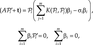
one attains the optimal values for A, t, and β_i (a vector of weights to be calculated for each correspondence), with K(x, y) = k Id being a d × d matrix where k ∝ e^{‖x − y‖}. The optimal transformation is then computed as $U (x_{i}) = \sum_{i = 1}^{m} K ({x,x}_{i}) β_{i}$ $U (x_{i}) = \sum_{i = 1}^{m} K ({x,x}_{i}) β_{i}$ . Another closed-form approach for affine registration is to reduce the affine problem to that of the orthogonal case [51]. However, the accuracy of this approach is questioned in [35].

When correspondences between extracted point sets are not known, rough estimation of the translation and rotation parameters can be done independently by first computing the displacement vector that would align the centroids of the point sets and then resolving for the rotation parameters via principal axis transform [18]. Spectral algorithms may also be used to solve rigid registrations, for example [58]. These algorithms operate by encoding point sets as affinity matrices and performing eigen-decomposition on these matrices. However, for spectral methods to work robustly, the eigen-structure of the affinity matrix must be rich in order to provide discriminating features for proper determination of point correspondences. Otherwise, optimization techniques such as the iterative closest point algorithm and its variants may be better alternatives [35].

Affine transformations may be solved in closed form using properties of the Fourier transform [125]. Furthermore, if U can be described by a finite set of displacement vectors, one may also solve for U by formulating a linear assignment problem (LAP) [130]. Recently, Westin et al. [64] also developed the polynomial expansion framework that was designed to solve global and local linear registrations analytically.

22.3.4.2 Iterative Optimization

A common approach taken by many optimization methods is to view the solution space as a 1D landscape, known as functional landscape, where a position on the landscape corresponds to a candidate solution and elevation corresponds to the optimality of a solution, that is, C. One then takes a step from the current to a new position on a path that would lead to the location of lowest elevation in the landscape. This can be mathematically expressed as

P_{k + 1} = P_{k} + a_{k} d_{k} (22.27)

$P_{k + 1} = P_{k} + a_{k} d_{k} (22.27)$

where P_k denotes a vector of transform parameters obtained in the current iteration, P_k+1 corresponds to a candidate vector to be examined next, d_k is the direction of the next step, and a_k is the size of the step.

There are many strategies for determining a_k. For example, it can simply be set to a fixed value. It can also be defined using a decaying function of k or a line search scheme where for every k, one tries to minimize C along the search direction d_k:

a_{k} = \arg \min_{a} C (P_{k} + a d_{k}) (22.28)

$a_{k} = \arg \min_{a} C (P_{k} + a d_{k}) (22.28)$

This can be costly as each iteration involves multiple evaluations of C, so inexact searches are usually used [67].

How one exactly computes d_k and a_k differentiates different optimization techniques from one and another. We next present two general classes of optimization methods: gradient-based and gradient-free. The former computes d_k based on the gradient of the cost function, typically by examining the cost function with regard to changes in transformation parameters. Conversely, gradient-free approaches operate on the cost function directly. The next subsections present the details of each.

22.3.4.2.1 Gradient-Based

Gradient-based methods may be deterministic or stochastic, where the difference lies in the use of a deterministic or random process during the entire optimization process [67].

Deterministic techniques that have been employed for image registration include gradient descent, quasi-Newton, nonlinear conjugate gradient, etc. These are common in that the search direction d_k is based on the derivative of the cost function with respect to the parameters. Under gradient descent techniques, the search direction is updated as

P_{k + 1} = P_{k} - a_{k} \frac{\partial C}{\partial P_{k}} (22.29)

$P_{k + 1} = P_{k} - a_{k} \frac{\partial C}{\partial P_{k}} (22.29)$

Klein et al. [66] explored two variants of the gradient descent method. One applies a decaying function on k for a_k; the other uses an inexact line search routine called “More-Thuente” to determine a_k.

Quasi-Newton (QN) methods may have “better theoretical convergence properties than gradient descent,” thanks to the use of second-order information [66]. They are based on the Newton–Raphson algorithm, which is given by

P_{k + 1} = P_{k} - {[H (P_{k})]}^{- 1} \frac{\partial C}{\partial P_{k}} (22.30)

$P_{k + 1} = P_{k} - {[H (P_{k})]}^{- 1} \frac{\partial C}{\partial P_{k}} (22.30)$

where H(P_k) is the Hessian matrix of the cost function. However, calculation of the inverse of the computation is expensive, so QN methods approximate the Hessian, for example, L = [H(P_k)]⁻¹. Calculation of L_k can be done in several ways, including Symmetric-Rank-1, Davidon–Fletcher–Powell, Broyden–Fletcher–Goldfarb–Shanno (BFGS), and the Limited memory BFGS, which is a variant of BFGS that avoids the need to store L in memory. According to [67], BFGS is very efficient in many applications.

The nonlinear conjugate gradient (NCG) method is based on the linear conjugate gradient method, which was first designed for solving a system of linear equations. NCG is an extension that is suitable for minimizing nonlinear functions. Under NCG, the search direction is defined as a linear combination of the cost gradient and the previous search direction, that is,

d_{k} = - \frac{\partial C}{\partial P_{k}} + β_{k} d_{k - 1} (22.31)

$d_{k} = - \frac{\partial C}{\partial P_{k}} + β_{k} d_{k - 1} (22.31)$

where the scalar β_k affects the convergence property and can be computed using different equations (see examples in [67]).

All of the aforementioned methods require an exact calculation or close approximation of the first- or second-order functional gradient. This can be very computational expensive. To address this, approximation of the cost gradient using stochastic sampling is done. The Kiefer–Wolfowitz method, for instance, uses finite difference to approximate the gradient, that is, $\tilde{g} \approx \partial / \partial P_{k}$ $\tilde{g} \approx \partial / \partial P_{k}$ [67]. This method requires 2N evaluations of the cost function for each k where N is the dimensionality of the solution space. The simultaneous perturbation method may also be used, which only performs two evaluations of the cost function, independent of N. The Robbins-Monro algorithm approximates the functional derivative using only a small subset of voxels randomly selected in every iteration. It was shown to give best compromise between convergence and accuracy over all aforementioned methods (both deterministic and stochastic ones), as evaluated in various registration experiments [67]. For further details on the aforementioned or other gradient-based optimization algorithms, we refer readers to Klein's thesis [67].

22.3.4.2.2 Gradient-Free

Next, we present different classes of gradient-free approaches, many of which make few or no assumptions about the problem being optimized and can conduct searches in a very large solution space. Often, some form of stochastic procedures is used in these methods.

22.3.4.2.2.1 Search Approaches

Powell's method (Powell's conjugate gradient descent method) is one commonly used gradient-free, search-based optimization technique. It finds the optimum in a d-dimensional solution space with a series of 1D searches. For example, finding the optimal parameters for an affine 3D transformation usually starts with a 1D search along lateral translation direction, then along the cranial–caudal translation direction, and followed by a rotation about each of the three axes. The choice of ordering influences the success of optimization and many have adopted heuristics to select the most suitable order.

A related algorithm is the simplex algorithm (aka Nelder-Mead simplex, downhill simplex, or amoeba method). Following the analogy of [144], one can see simplex as a creature with n + 1 feet crawling in an n-D search space. One of its feet stands on the initial parameter estimate while the rest are randomly placed. At each iteration, the cost function is evaluated at each foot position and the foot with the worst cost is moved to improve its cost. Some specific rules are designed to guide which foot to move next and by how much.

Other examples of search-based algorithms include simulated annealing, DIRECT [135], and Tabu search.

22.3.4.2.2.2 Evolutionary Algorithms

A representative class of metaheuristics is evolutionary algorithms (EAs). EAs are based on the principle of natural selection, that is, the fittest survives. The solution space is seen as a dynamic population. A candidate solution plays the role of an individual in a population and its function cost corresponds to its fitness value of surviving in the population. Evolution of the population then occurs after repeated applications of reproduction (aka inheritance), mutation, recombination (aka crossover), and selection. Many methods based on this idea have been proposed in the literature; an extensive review is given in [31].

One popular choice is the evolutionary strategy (ES). In each iteration, “children” are created via mutation of the population (its “parents”). A mutation is a random vector generated from a multidimensional normal distribution. The covariance matrix of the distribution is adapted in each iteration: it is increased if the new population consists of better individuals or decreased otherwise. The population then reduces back to its original size by keeping only the fittest. A variant is the one-plus-one ES [115], where both the population size and the number of children generated are equal to 1; this variant was used by Chillet et al. [24] to affinely register 3D models of brain and liver vasculatures (encoded with an inverted distance map) to CT or MR images.

A relatively new class of algorithms for multimodal function optimization is those based on artificial immune systems (AIS), which are inspired by theoretical immunologic models. They are capable of locating the global minimum of a function as well as a large number of strong local optima by automatically adjusting the population size and combining local with global searches. Recently, Delibasis et al. [33] applied it to solve for a spatial matching between point correspondences identified in medical images.

Of all EA methods, the current state-of-the-art is probably the covariance matrix adaptation method [67]. It has several phases. In the reproduction phase, a set of m search directions (d_k) is generated from a normal distribution whose covariance matrix is computed to favor search directions that were successful in previous iterations (and m is a user-defined parameter controlling the population size). In the selection phase, the cost function is evaluated for each search direction using Equation 22.28, and the l best search directions are selected. Finally, in the recombination phase, a weighted average of the l selected trial directions is computed to generate the next set of search directions. Recommendations for the choice of m and l based on n are given in [67].

22.3.4.2.2.3 Discrete Optimization

Discrete optimization operates by searching for the best solution out of a discrete set of solutions. When applied to image registration, they usually involve modeling the deformation U as a random field and recasting registration of F and M as a Markov Random Field (MRF) energy minimization problem [14,46,71,109], which formulates the statistical dependence between F and M as

p (F, U | M) = p (F | U, M) p (U) . (22.32)

$p (F, U | M) = p (F | U, M) p (U) . (22.32)$

where the conditional probability p(F|U, M) is the data likelihood that models dependence between intensity values between the two images and the prior probability p(U) is the prior that favors plausible deformations. As we will see shortly, these probabilities essentially correspond to data dissimilarity and regularization terms of a typical registration objective given in Equation 22.7. Assume F is conditionally independent of U and M, the first term in the preceding becomes

p (F, U | M) = \underset{x \in Ω}{\prod^{​}} p (F (x) | U (x), M (x)) . (22.33)

$p (F, U | M) = \underset{x \in Ω}{\prod^{}} p (F (x) | U (x), M (x)) . (22.33)$

Assuming further that F(x) only depends on M ° U(x) and not the rest of the values in M, one obtains

p (F (x) | U (x), M (x)) = p (F (x) | M \circ U (x)) (22.34)

$p (F (x) | U (x), M (x)) = p (F (x) | M \circ U (x)) (22.34)$

We will now see how use of discrete optimization can simplify maximum a posterior (MAP) inference. Let the spatial coordinates of M be a graph G (whose set of nodes V correspond to x ∊ Ω and edges (x_i, x_j) ∊ ∊ encode neighborhood relationships, for example, 4-connectivity in 2D, etc.). In the simplest form, the data likelihood can model pixel-wise dependence between F and M with a Gaussian noise model, that is,

p (F | M \circ U)) = \underset{x_{i} \in v}{\prod^{​}} p (F (x_{i}) | M (U (x_{i}))) = \underset{x_{i} \in v}{\prod^{​}} e^{- 0.5 {(F (x_{i}) - M (U (x_{i})))}^{2}}; (22.35)

$p (F | M \circ U)) = \underset{x_{i} \in v}{\prod^{}} p (F (x_{i}) | M (U (x_{i}))) = \underset{x_{i} \in v}{\prod^{}} e^{- 0.5 {(F (x_{i}) - M (U (x_{i})))}^{2}}; (22.35)$

and the prior can be encoded as a regularization penalty that examines the interactions between displacements of two neighboring points x_i, x_j, that is,

p (U) = \underset{(x_{i}, x_{j}) \in ε}{\prod^{​}} {‖ U (x_{i}) - U (x_{j}) ‖}^{2} (22.36)

$p (U) = \underset{(x_{i}, x_{j}) \in ε}{\prod^{}} {‖ U (x_{i}) - U (x_{j}) ‖}^{2} (22.36)$

Performing MAP inference can now be done as minimization of the following:

E (U) = - p (F, U | M) = - \prod_{x_{i} \in ν} p (F (x_{i}) | M (U (x_{i}))) p (U (x_{i})) (22.37)

$E (U) = - p (F, U | M) = - \prod_{x_{i} \in ν} p (F (x_{i}) | M (U (x_{i}))) p (U (x_{i})) (22.37)$

which leads to minimization of the following MRF energy:

- \log (E (U)) = \sum_{x_{i} \in ν} \underset{θ_{i}}{\underset{︸}{{(F (x_{i}) - M (U (x_{i})))}^{2}}} + \sum_{(x_{i}, x_{j}) \in ε} \underset{θ_{i j}}{\underset{︸}{{‖ U (x_{i}) - U (x_{j}) ‖}^{2}}} (22.38)

$- \log (E (U)) = \sum_{x_{i} \in ν} \underset{θ_{i}}{\underset{︸}{{(F (x_{i}) - M (U (x_{i})))}^{2}}} + \sum_{(x_{i}, x_{j}) \in ε} \underset{θ_{i j}}{\underset{︸}{{‖ U (x_{i}) - U (x_{j}) ‖}^{2}}} (22.38)$

where the first summation over unary potentials θ_i is identical to the SSD metric (Section 22.3.3) and the second summation over pair-wise potentials θ_ij resembles a Laplacian regularizer on U (Section 22.3.2). Note that this MRF energy contains potentials of first-order^* and that the maximum clique of its corresponding graph is size of 2.

MAP inference with MRF as given earlier can be solved with different classes of algorithms; these include linear programming, message passing, and graph-cut. Algorithms for solving integer linear programs include cutting-plane method, branch-and-bound, branch-and-cut, etc. Message passing algorithms include Belief Propagation, Tree Reweighted Message Passing (TRMP), and Max-Product algorithms. Graph-cut algorithms include α-expansion and α-β swap [14].

Different matching problems have adopted a discrete optimization approach [14,70]. For MIR, one of the earliest applications of MRF energy minimization include [121] where Tang and Chung resolved U at every location via minimization of Equation 22.38. Lombaert et al. [79] later extended [120] by incorporating the use of landmarks for deformable registration of coronary angiograms.

To control deformations more effectively, Glocker et al. [46] parameterized U with FFD transformation model and applied MAP inference to solve for the optimal translations of the control points of the B-spline model. To minimize their objective function, they employed Fast-PD [69] (stands for Fast Primal-Dual approximation), which works by solving the energy minimization problem by a series of graph-cut computations. The process reuses the primal and dual solutions of the linear programming relaxation of the energy minimization problem obtained in the previous iteration, thus effectively decreases run time; see review [47] for details. Their method was widely accepted due to its high efficiency and public availability made possible through their software called DROP, which contains implementations of various image similarity measures. Kwon et al. [71] also used the FFD framework for 2D registration, but proposed the following higher-order regularization term that does not penalize global transformations like Equation 22.38 would:

\sum_{(x_{i}, x_{j}, x_{k})} \sum_{d = {1, 2}} {‖ - U_{d} (x_{i}) + 2 U (x_{j}) - U_{d} (x_{k}) ‖}^{2} (22.39)

$\sum_{(x_{i}, x_{j}, x_{k})} \sum_{d = {1, 2}} {‖ - U_{d} (x_{i}) + 2 U (x_{j}) - U_{d} (x_{k}) ‖}^{2} (22.39)$

where U_d denotes the dth component of U. The higher-order MRF energy was then converted to a pair-wise one, so it could be solved with TRWP.

In [109], Shekhovtsov et al. performed MRF-based matching using a linear programming relaxation technique. However, they proposed to decompose a 2D deformation model into x and y components so that the problem could be solved with sequential TRMP. Lastly, Lempitsky et al. [74] proposed the fusion-move approach to combine discrete optimization with continuously valued solutions for 2D image registration, effectively avoiding local minima while avoiding problems due to discretizing the deformation space. Specifically, candidate flow fields (Û) were generated using the method of [53]. Each candidate flow was seen as a “proposal” label l ∊ ℒ, which was then iteratively examined and fused in a moving-making approach. MRF-energy minimization in each iteration was performed with the Quadratic Pseudo Boolean Optimization algorithm [68]. In regularizing U, the authors proposed the following pair-wise potentials:

θ_{i j} = \sum_{d = 1, 2} ρ (\frac{U_{d} (x_{i}) - U_{d} (x_{i})}{‖ x_{i} - x_{j} ‖}) (22.40)

$θ_{i j} = \sum_{d = 1, 2} ρ (\frac{U_{d} (x_{i}) - U_{d} (x_{i})}{‖ x_{i} - x_{j} ‖}) (22.40)$

where $ρ (x) = \log (1 + \frac{1}{2 b^{2}} x^{2})$ $ρ (x) = \log (1 + \frac{1}{2 b^{2}} x^{2})$ and b is a constant. Fused solutions were then refined with gradient-based optimization.

22.4 Two Commonly Adopted Registration Paradigms

22.4.1 Demons Algorithm and Its Extensions

To better understand thermodynamic equilibrium, the Scottish physicist James Maxwell [123] came up with the concept of demons as door guards that selectively allow “hot” molecules through. Adopting this concept, Thirion [123] proposed to formulate registration as a process where demons locally push voxels into or out of object boundaries to allow for image matching, by treating images as isointensity contours and computing demon forces to push these contours in their normal direction to encourage image alignment. The orientation and magnitude of the forces are derived from the instantaneous optical flow equation [56], which assumes that M is the deformed F, whose deformations δx are due to local motions that occur after δt, that is,

\begin{array}{l} M (x) = F (x + δ x, t + δ t) \\ F (x, t) - F (x + δ x, t + δ t) = 0 \end{array}

$\begin{array}{l} M (x) = F (x + δ x, t + δ t) \\ F (x, t) - F (x + δ x, t + δ t) = 0 \end{array}$

Images

where the last equation is known as the brightness constancy assumption. Using linear approximation, we get,

\begin{matrix} F (x + δ x, t + δ t) = F (x, t) + \frac{\partial F}{\partial x} δ x + \frac{\partial F}{\partial t} δ t \\ 0 = \frac{\partial F}{\partial x} \frac{δ x}{δ t} + \frac{\partial F}{\partial t} δ t (known as the optical flow constraint) \\ - \frac{\partial F}{\partial t} δ t = \nabla F \frac{δ x}{δ t} \\ - (M (x) - F (x)) = \nabla F (x) V (x) \end{matrix}

$\begin{matrix} F (x + δ x, t + δ t) = F (x, t) + \frac{\partial F}{\partial x} δ x + \frac{\partial F}{\partial t} δ t \\ 0 = \frac{\partial F}{\partial x} \frac{δ x}{δ t} + \frac{\partial F}{\partial t} δ t (known as the optical flow constraint) \\ - \frac{\partial F}{\partial t} δ t = \nabla F \frac{δ x}{δ t} \\ - (M (x) - F (x)) = \nabla F (x) V (x) \end{matrix}$

Images

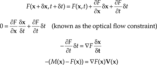
The method alternates between computing the image forces and performing regularization on the motion field using Gaussian smoothing. This simple scheme is computationally efficient. In [97], Pennec et al. showed that the Demons algorithm can be seen as an approximation of a second-order gradient-descent on the SSD metric. Bro-Nielsen [17] also showed that applying the Gaussian filter instead of the real linear elastic filter is an approximation of the fluid model; see details in Section 22.3.2.2.2. Surveys of the state of art of optical flow algorithms are given in [10,135] and the references therein; the latter in particular also provides public data sets and methodologies for evaluation of optical flow algorithms. [75] also provides ground truth motion fields of real-world videos.

Since its conception, different extensions of Thirion's Demons algorithm were proposed; these include extension of the image forces to be based on cross-correlation [5] or phase [59]. In [19], Cachier et al. proposed the PASHA algorithm, which incorporates the addition of a random field C (essentially, an “intermediate transformation” [85]) to allow for inexact point correspondences as given by U. This leads to minimization of the following energy

E (C, U) = \frac{1}{γ_{n}} {‖ F - M \circ C ‖}^{2} + \frac{1}{γ_{c}} {‖ C - U ‖}^{2} + \frac{1}{γ} {‖ \nabla U ‖}^{2} (22.41)

$E (C, U) = \frac{1}{γ_{n}} {‖ F - M \circ C ‖}^{2} + \frac{1}{γ_{c}} {‖ C - U ‖}^{2} + \frac{1}{γ} {‖ \nabla U ‖}^{2} (22.41)$

where the first term measures the quality of the field of point correspondence C between the deformed M and F based on a data dissimilarity measure; γ_n accounts for the noise in the image, γ_c accounts for spatial uncertainty on the correspondences, and γ controls the amount of regularization on U. Rather than solving the complex energy minimization in Equation 22.46, Cachier et al. alternatively optimize Equation 22.46 with regard to C given U, and then optimize Equation 22.46 with regard to U given C. The second optimization has a closed-form solution when the regularization is quadratic and uniform, and can be obtained by setting it as the convolution of C by a Gaussian kernel [132].

To solve the first optimization, that is, minimize $\frac{1}{γ_{n}} {‖ F - M \circ C ‖}^{2} + \frac{1}{γ_{c}} {‖ C - U ‖}^{2}$ $\frac{1}{γ_{n}} {‖ F - M \circ C ‖}^{2} + \frac{1}{γ_{c}} {‖ C - U ‖}^{2}$ with regard to C given U, one linearly approximates the data (first) term for every pixel as

ψ (x) = F (x) M (x) \circ U \circ C (x) \approx F (x) - M (x) \circ U (x) + I (x) \circ C (x) (22.42)

$ψ (x) = F (x) M (x) \circ U \circ C (x) \approx F (x) - M (x) \circ U (x) + I (x) \circ C (x) (22.42)$

where J(x) = − ∇M° U(x). This allows one to rewrite the first optimization as

E (C | U) \approx \frac{1}{2 | Ω |} \underset{x \in Ω}{\sum^{​}} {‖ [\begin{matrix} F - M \circ U (x) \\ 0 \end{matrix}] + [\begin{matrix} J (x) \\ \frac{γ_{n} (x)}{γ_{c}} I \end{matrix}] C (x) ‖}^{2} (22.43)

$E (C | U) \approx \frac{1}{2 | Ω |} \underset{x \in Ω}{\sum^{}} {‖ [\begin{matrix} F - M \circ U (x) \\ 0 \end{matrix}] + [\begin{matrix} J (x) \\ \frac{γ_{n} (x)}{γ_{c}} I \end{matrix}] C (x) ‖}^{2} (22.43)$

where γ_n(x) = |F(x) − M ° C(x)| is a local estimation of noise that is used. Since the approximation for each pixel is independent of each other, one instead solves a simple system for each pixel using the following normal equation:

(J^{T} (x) J (x) + \frac{γ_{n}}{γ_{c}} I) C (x) = - (F (x) - M \circ U (x)) J^{T} (x) (22.44)

$(J^{T} (x) J (x) + \frac{γ_{n}}{γ_{c}} I) C (x) = - (F (x) - M \circ U (x)) J^{T} (x) (22.44)$

C (x, F, M) = - \frac{F (x) - M \circ U (x)}{{‖ J (x) ‖}^{2} + \frac{γ_{n}^{2} (x)}{γ_{c}^{2}}} J^{T} (22.45)

$C (x, F, M) = - \frac{F (x) - M \circ U (x)}{{‖ J (x) ‖}^{2} + \frac{γ_{n}^{2} (x)}{γ_{c}^{2}}} J^{T} (22.45)$

All of this leads to the following modified demons algorithm:

Start with an initial estimate of Û.
Compute an update for C as given in Equation 22.45.
To enforce fluid-like regularization (Section 22.3.2.2), set C ← K ^* C, where K is generally a Gaussian kernel.^* Otherwise, skip this step.
Compute C ← U + C.
- To enforce elastic-like regularization, compute U ← K * C.
- Otherwise, compute U ← C.

where the convolution of C with a Gaussian kernel is an efficient approximation to elastic or fluid regularization.

To spatially adapt regularization, Stefanescu et al. [114] smoothed U using a variable Gaussian kernel whose size depended on a scalar field that encoded the expected amount of deformations as estimated from prior segmentation of the anatomy. The authors also filtered C after each iteration according to a measure that is based on local intensity variance and gradient.

Yet another extension is called the Log Domain Diffeomorphic Demons (LDDD), which was proposed by Vercauteren et al. [131,133] to constrain U to reside in the space of diffeomorphisms Diff(Ω). Recall that when performing an n-dimensional optimization search in ℛⁿ, the iterative step used in Newton's optimization method is of the form P_k+1 = P_k + a_kd_k, where d_k is the descent direction, which lies in the tangent space of ℛⁿ. ⁿ to the space of diffeomorphisms (i.e., smooth manifold), the descent direction that lies in the tangent space at P_k is different from the tangent spaces of any other point. To map a point on the tangent space of P_k to a point on the manifold, one thus employs the exponential map operation, that is, exp: V↦ Diff(Ω). Accordingly, parameter-izing U and C by stationary velocity fields V and V_C via exponential map, that is, U = exp(V), C = exp(V_C), one now minimizes the log-domain version of Equation 22.46 with regard to V_C:

E (C, U) = \frac{1}{γ_{n}} {‖ F - M \circ \exp (V_{C}) ‖}^{2} + \frac{1}{γ_{c}} {‖ l o g (\exp (- V) \circ \exp (V_{C})) ‖}^{2} + \frac{1}{γ} ‖ \nabla V ‖^{2} . (22.46)

$E (C, U) = \frac{1}{γ_{n}} {‖ F - M \circ \exp (V_{C}) ‖}^{2} + \frac{1}{γ_{c}} {‖ l o g (\exp (- V) \circ \exp (V_{C})) ‖}^{2} + \frac{1}{γ} ‖ \nabla V ‖^{2} . (22.46)$

The iterative update in the aforementioned step 4 becomes

C \leftarrow U \circ \exp (δ v), (22.47)

$C \leftarrow U \circ \exp (δ v), (22.47)$

where δv is a small update velocity field that was derived in [84] as $\frac{F (x) - M \circ U (x)}{{‖ J (x) ‖}^{2} + \frac{γ_{n}^{2}}{γ_{c}^{2}}} J (x)$ $\frac{F (x) - M \circ U (x)}{{‖ J (x) ‖}^{2} + \frac{γ_{n}^{2}}{γ_{c}^{2}}} J (x)$ .

To further enforce inverse consistency (Section 22.3.2.4.1), Vercauteren et al. further proposed a symmetric version of LDDD [132]. Other extensions of the demons algorithm include multichannel diffeomorphic demons [99]; spherical demons, which operates on the sphere for surface registration [153]; as well as iLogDemons [85], which incorporates elasticity and incompress-ibility constraints.

22.4.2 block-Matching and HAMMER

Block-matching (BM) is an efficient scheme for isolating and selecting salient parts of an image to drive the process of registration. Usually, a BM algorithm consists of the following steps that iterate until certain convergence criterion is met. First, blocks of image pixels computed from F and M are matched according to their similarity scores and displacement vectors are computed from the best matches. Second, displacements of all voxels in the entire domain are then computed from the matches via interpolation, for example, using TPS [84] or a Gaussian weighting scheme [111]. Then, regularization on U is subsequently enforced via Gaussian filtering on U.

This matching method was originally proposed for video sequence^* matching but has been successfully used for MIR since its first adoption in [32] by Collins et al. Some of its successful applications include elastic registration of neck-and-head, paraspine, and prostate images as performed in [84] (where blocks belonging to detected anatomical landmarks were matched based on local cross-correlation), as well as piecewise affine registration of biological images (e.g., histological sections, autoradiographs, cryosections, etc.) as performed in [100] (where robust least square was used to estimate the local transformations associated to each matching pair).

Both demons framework and BM algorithms are quite similar in that both perform regularization of U via post-filtering (i.e., apply filtering on update of U per iteration). However, rather than computing the data forces for all voxels, BM involves an additional/explicit step of preselecting salient regions only in which data forces are calculated for matching. Unlike the original demons algorithm, BM algorithms are also capable of recovering large deformations thanks to the strategy of matching blocks of different scales hierarchically (e.g., start with large blocks, then reduce their sizes in subsequent stages). For example, it was shown capable of recovering rotations up to 28° in a study involving rat brain sections (see details in [100]).

One frequently cited BM-based registration framework is called HAMMER, which stands for Hierarchical Attribute Matching Mechanism for Elastic Registration. First proposed in [111] by Shen and Daatziko, important voxels or driving voxels are selected based on the attribute vectors (AV) (Section 22.3.3) computed from each voxel. The selection of voxels and their influences on the current estimate of U are hierarchically determined. Specifically, in the early stages of registration, the similarity between two driving voxels is determined based on the weighted sum of the AV similarities in the subvol-umes that encompass each of the two voxels. A match occurs only when the integrated similarity is beyond a user-defined threshold, which is initially set to a high value. The threshold as well as the size of the subvolumes are then decreased at a user-defined rate in each iteration.

Some of the later extensions and applications of HAMMER include the following:

Optimize parameters that define the set of AVs [145]
Use of local spatial intensity histogram [110] or wavelets [150] to define the AVs
Incorporation of landmark correspondences for matching, and replace Gaussian with TPS for interpolation of U [147]
Groupwise registration using HAMMER [148]

22.5 Evaluating Registrations

A logical start on evaluating registration results is to examine them subjectively. For images of the same modality, one can visualize the results by examining the registered images individually on separate windows with a linked cursor (“split window validation” [86]), examining their checker-board or difference image, or viewing them jointly with alpha-bending.^* For images of different modality, the alpha-bending is the most common tool as all image characteristics in both images can be displayed simultaneously [119]. Furthermore, if segmentation of one or both of the two images is available, one can also overlay the segmentation contours of one image on top of the image to be matched to; see [16] for examples.

In general, due to limits of subjective evaluation,^{^†} qualitative approaches are also guided with quantitative evaluation.

Quantitative evaluation of a registration technique may be broadly classified in terms of the nature of the experiment: synthetic or real.

Validation based on synthetic data is generally conducted in a controlled setting, usually performed to evaluate particular components of a registration method. For example, when performing registration with gradient-based optimization, one often examines the “smoothness” and the capture range of the metric (by computing the metric between two images with regard to a range of misalignments). One may also examine the robustness of an algorithm, that is, registration results remain reasonable even in extreme scenarios. A formalized protocol involving the aforementioned measures on a given image pair with known “ground truth” registration is given in [112]. One may also examine an algorithms’ performance by studying its inverse consistency and transitivity (i.e., registration results transfer, e.g., propagating registration result from A to B to C to B, and then back to A should yield zero in the composition of all obtained deformations maps [13]).

For mono-modality registration, where one assumes that M is a deformed version of F with additive noise corruption, one common practice to quantify registration quality is to compute the mean square error (MSE) between the deformed moving image and fixed image. MSE may further be used to compute the Peak-Signal-to-Noise Ratio (PSNR), which equals to $10 l o g (I_{\max}^{2} / M S E)$ $10 l o g (I_{\max}^{2} / M S E)$ where I_max is the maximum intensity between two images. The PSNE is a common measure to evaluate image reconstruction quality, and has been used in [134] to measure registration accuracy. However, an implausible warp may always produce zero MSE. Generally, examining intensity values alone does not evaluate the plausibility and quality of U and so both MSE and PSNR should not be the sole quantitative measurements.

A more direct and arguably more complete evaluation approach is to examine an algorithm's ability to recover known misalignments. Starting with a pair of images, subjectively judged as registered, one then applies random misalignments and/or warps to one of the pair [61]. Then, a registration error metric (e.g., angular error or mean Euclidean distance) is computed to measure the residual between the obtained transform and the known transform (that misaligned the original pair) within the region of interest. Countless works, for example [10,46,71,109,117,118,121,140,157–159], have adopted this approach.

Validation based on real data involves performing actual image registrations and employing additional data, ideally provided by clinical experts, to quantify accuracy of the obtained results. For example, if landmark correspondences can be acquired, one may compute the target registration error (TRE) [141]. However, in order for precise assessment, it is important that the correspondences are as spatially distributed as possible, especially for results obtained from deformable registration. If segmentation of the images is available, one can also apply the warp to the segmentation and compute overlap measures^* between the target and deformed segmentations. The latter approach is known as morphology-based evaluation [5,66].

Several issues evolve around landmark-based and morphology-based evaluations. First, acquiring additional validation data is difficult and laborious. For instance, landmarking 3D images (usually using 2D displays) is a challenging task due to limited sense of spatial context and depth. And when one or both of the input images are functional data (e.g., PET or SPECT, where anatomical boundaries cannot be reliably segmented automatically or manually), it becomes extremely difficult [136], if not impossible. Second, low interoperator variability^{^†} of the segmentation/landmarking results cannot always be guaranteed. To reduce variability that may be introduced by operator's biases and experience, protocols have been established for segmentation, for example, brain images [66], and for identification of anatomical landmark, for example, femur [108]. Third, morphology-based evaluation does not provide a complete insight of registration accuracy. One problem is that quantitation cannot be expressed in a unit that is relevant for task of registration (e.g., distance in mm). Another is that it focuses only on segmented regions and disregards unsegmented structures as well as the regions within or surrounding the segmented regions.

Due to the aforementioned factors, evaluation based on segmentations are usually regarded as “bronze” evaluation, suggesting that one should interpret with caution.

In the MIR literature, numerous researchers have performed comparative studies to evaluate a set of registration algorithms that have been designed for different problems. The earliest work is the Nonrigid Image Registration Evaluation Project (NIREP), which standardized a set of benchmarks and metrics (overlap, variance of image intensities in a population of registered images,^{^‡} transitivity, and inverse consistency). The initial phase of NIREP involved a data set of 16 labeled brain images. Other comparative analyses include study of [128], where Urschler et al. compared six deformable registration algorithms with an experiment involving synthetic deformations applied to two pairs CT lung images.

Recently in 2010, Murphy et al. [94] have set up a web-based public platform called EMPIRE to allow for a “fair and meaningful comparison of registration algorithms applied to thoracic CT data.” The website allows developers to download image pairs and upload the corresponding registrations they obtained for evaluation as performed by the website. Four sets of measures are then later reported on the site, which include those based on alignment of lung boundary and fissures. As of October 2011, over 30 teams have submitted their results to this website.

For brain image, comparative studies in which at least three nonlinear algorithms were compared on whole-brain registrations that have been completed in the last decade include:

Studies by Hellier et al. (see [66]): A series of publications that compared five nonlinear methods that focused on registration accuracy in the cortical areas. Two sets of evaluation measures were used, including segmentation overlap, deformation quality (amount of singularities present), and symmetric hausdorff distance between segmented sulci surfaces. The authors also examined results in terms of shape similarity using PCA.
Study by Yassa and Stark [152]: Six algorithms and two semi-automated methods were compared based on two measures (overlap and “measure of blur” similar to intensity variance) computed in the cortical areas. They remarked that their evaluation involving 18 images could not affirm that the nonrigid methods they examined can perform better in registering major cortical sulci.
Study of Klein et al. [66]: the study compared 14 registration algorithms using four data sets by performing over 2168 image registrations per algorithm and computing various evaluation measures and performing statistical analyses on the obtained evaluation measures. Top-ranking methods were SyN (Symmetric Normalization) [8]), ART^*, IRTK [105], and SPM's DARTEL toolbox [4], with the first two giving top scores in all tests and for all label sets. SyN is recommended if high accuracy is desired; ROMEO^{^†} and Diffeomorhpic Demons [131] are more efficient alternatives for time-sensitive tasks.

22.6 Conclusions

This chapter reviewed the various techniques proposed for MIR, as well as those relating to registration evaluation. In summary, key tasks of a registration procedure include (1) characterization of the registration solution Section 22.3.2; (2) definition of one or a set of criterion to quantify the optimality of the solution (Section 22.3.3; and (3) design and employment of an optimization strategy for finding the solution (Section 22.3.4.2). As there is currently no generic registration algorithm that works in all applications, choices of data (dis)similarity terms and optimization strategy remain highly problem-specific.

There remain many open questions in MIR. For instance, MIR is challenged by the need for tuning a potentially long list of parameters that relate to optimization and feature extraction settings, as well as the weights between data dissimilarity and regularization terms. Furthermore, when operated on large images (e.g., vector- or tensor-valued images and dynamic sequences), MIR is burdened by heavy computation and memory demands. Future research works that aim at addressing these issues are therefore both interesting and important.

References

1. O. Acosta, J. Fripp, A. Rueda, D. Xiao, E. Bonner, P. Bourgeat, and O. Salvado. 3D shape context surface registration for cortical mapping. In Proceedings of the 2010 IEEE International Conference on Biomedical Imaging: From Nano to Macro, ISBI’10, IEEE Press, Piscataway, NJ, 2010, pp. 1021–1024.

2. A. Pluim, J. Maintz, and M. Viergever. Mutual information based registration of medical images: A survey. IEEE Transactions on Medical Imaging, 21:61–75, 2003.

3. V. Arsigny, X. Pennec, and N. Ayache. Polyrigid and polyaffine transformations: A new class of diffeomorphisms for locally rigid or affine registration. In Proceedings of MICCAI, Springer, Heidelberg, Germany, 2003, pp. 829–837.

4. J. Ashburner. A fast diffeomorphic image registration algorithm. Neuroimage, 38(1):95–113, 2007.

5. B. Avants, C. Epstein, M. Grossman, and J. Gee. Symmetric diffeomorphic image registration with cross-correlation: Evaluating automated labeling of elderly and neurodegenerative brain. Medical Image Analysis, 12(1):26–41, 2008. Special Issue on The Third International Workshop on Biomedical Image Registration—WBIR 2006.

6. B. Avants, N. Tustison, and G. Song. Advanced normalization tools: V1.0. Insight Journal, http://hdl.handle.net/10380/3113, July 2009.

7. B. B. Avants, P. T. Schoenemann, and J. C. Gee. Lagrangian frame diffeomor-phic image registration: Morphometric comparison of human and chimpanzee cortex. Medical Image Analysis, 10(3):397–412, 2006. Special Issue on The Second International Workshop on Biomedical Image Registration (WBIR’03).

8. B. B. Avants, N. J. Tustison, G. Song, P. A. Cook, A. Klein, and J. C. Gee. A reproducible evaluation of ANTS similarity metric performance in brain image registration. Neuroimage, 54(3):2033–2044, 2011.

9. A. Azar, C. Xu, X. Pennec, and N. Ayache. An interactive hybrid non-rigid registration framework for 3D medical images. In Third IEEE International Symposium on Biomedical Imaging: Nano to Macro, 2006, Paris, France, April 2006, pp. 824–827.

10. S. Baker, D. Scharstein, J. P. Lewis, S. Roth, M. J. Black, and R. Szeliski. A database and evaluation methodology for optical flow. International Journal of Computer Vision, 92(1):1–31, 2011.

11. M. Beg and A. Khan. Symmetric data attachment terms for large deformation image registration. IEEE Transactions on Medical Imaging, 26(9):1179–1189, September 2007.

12. M. F. Beg, M. I. Miller, A. Trouvé, and L. Younes. Computing large deformation metric mappings via geodesic flows of diffeomorphisms. International Journal of Computer Vision, 61:139–157, February 2005.

13. E. T. Bender and W. A. Tomé. The utilization of consistency metrics for error analysis in deformable image registration. Physics in Medicine and Biology, 54(18):5561, 2009.

14. Y. Boykov and V. Kolmogorov. An experimental comparison of min-cut/max-flow algorithms for energy minimization in vision. In Proceedings of the Third International Workshop on Energy Minimization Methods in Computer Vision and Pattern Recognition, EMMCVPR ‘01, Springer-Verlag, London, U.K., 2001, pp. 359–374.

15. M. Bro-Nielsen. Medical image registration and surgery simulation. PhD thesis, IMM-DTU, 1996.

16. M. Bro-Nielsen. Rigid registration of CT, MR and cryosection images using a GLCM framework. In J. Troccaz, E. Grimson, and R. Mösges, eds., CVRMed-MRCAS’97, vol. 1205 of Lecture Notes in Computer Science, Springer, Berlin, Germany, 1997, pp. 171–180. 10.1007/BFb0029236.

17. M. Bro-Nielsen and C. Gramkow. Fast fluid registration of medical images. In Proc. Visualization in Biomedical Computing (VBC’96), September, Springer Lecture Notes in Computer Science, Hamburg, Germany, vol. 1131, 1996, pp. 267–276.

18. L. G. Brown. A survey of image registration techniques. ACM Computing Surveys, 24:325–376, December 1992.

19. P. Cachier, J.-F. Mangin, X. Pennec, D. Rivière, D. Papadopoulos-Orfanos, J. Régis, and N. Ayache. Multisubject non-rigid registration of brain MRI using intensity and geometric features. In Proceedings of MICCAI, Utrecht, the Netherlands, 2001, pp. 734–742.

20. N. D. Cahill, J. A. Noble, and D. J. Hawkes. A demons algorithm for image registration with locally adaptive regularization. In Proceedings of the 12th International Conference on Medical Image Computing and Computer-Assisted Intervention: Part I, MICCAI ‘09, Springer-Verlag, Berlin, Germany, 2009, pp. 574–581.

21. K. Cao, K. Ding, G. E. Christensen, M. L. Raghavan, R. E. Amelon, and J. M. Reinhardt. Unifying vascular information in intensity-based nonrigid lung CT registration. In WBIR, Springer-Verlag, Berlin, Germany, 2010, pp. 1–12.

22. F. Chen and D. Suter. Image coordinate transformation based on div-curl vector splines. In ICPR’98, IEEE Computer Society Press, Brisbane, QLD, Australia, 1998, pp. 518–520.

23. W. Cheung and G. Hamarneh. n-sift: n-dimensional scale invariant feature transform. IEEE Transactions on Image Processing, 18(9):2012–2021, September 2009.

24. D. Chillet, J. Jomier, D. Cool, and S. Aylward. Vascular atlas formation using a vessel-to-image affine registration method. In R. Ellis and T. Peters, eds., Medical Image Computing and Computer-Assisted Intervention—MICCAI 2003, vol. 2878 of Lecture Notes in Computer Science, Springer, Berlin, Germany, 2003, pp. 335–342.

25. G. Christensen, P. Yin, M. W. Vannier, K. Chao, J. F. Dempsey, and J. Williamson. Large-deformation image registration using fluid landmarks. In Fourth IEEE Southwest Symposium on Image Analysis and Interpretation, 2000, pp. 269–273.

26. G. E. Christensen and H. J. Johnson. Consistent image registration. IEEE Transaction on Medical Imaging, 20(7):568–582, 2001.

27. G. E. Christensen and H. J. Johnson. Invertibility and transitivity analysis for nonrigid image registration. Journal of Electronic Imaging, 12(1):106–117, 2003.

28. G. E. Christensen, S. C. Joshi, M. I. Miller, and S. Member. Volumetric transformation of brain anatomy. IEEE Transactions on Medical Imaging, 16:864–877, 1997.

29. G. E. Christensen, R. D. Rabbitt, and M. I. Miller. 3D brain mapping using a deformable neuroanatomy. Physics in Medicine and Biology, 39(3):609–618, 1994.

30. H. Chui, J. Rambo, J. Duncan, R. Schultz, and A. Rangarajan. Registration of cortical anatomical structures via robust 3D point matching. In A. Kuba, M. áamal, and A. Todd-Pokropek, eds., Information Processing in Medical Imaging, vol. 1613 of Lecture Notes in Computer Science, 1999, pp. 168–181.

31. C. A. C. Coello. A comprehensive survey of evolutionary-based multiobjective optimization techniques. Knowledge and Information Systems, 1:269–308, 1998.

32. D. L. Collins and A. C. Evans. ANIMAL: Validation and applications of nonlinear registration-based segmentation. IJPRAI, 11(8):1271–1294, 1997.

33. K. K. Delibasis, P. A. Asvestas, and G. K. Matsopoulos. Automatic point correspondence using an artificial immune system optimization technique for medical image registration. Computerized Medical Imaging and Graphics (in press).

34. M. Droske and M. Rumpf. Multiscale joint segmentation and registration of image morphology. IEEE Transactions on Pattern Analysis and Machine Intelligence, 29(12):2181–2194, December 2007.

35. S. Du, N. Zheng, S. Ying, and J. Liu. Affine iterative closest point algorithm for point set registration. Pattern Recognition Letters, 31(9):791–799, 2010.

36. D. Eggert, A. Lorusso, and R. Fisher. Estimating 3-d rigid body transformations: a comparison of four major algorithms. Machine Vision and Applications, 9:272–290, 1997. 10.1007/s00138005 0048.

37. A. El-Baz, A. Farag, G. Gimel'farb, and A. Abdel-Hakim. Image alignment using learning prior appearance model. In 2006 IEEE International Conference on Image Processing, Atlanta, Georgia, October 2006, pp. 341–344.

38. J. M. Fitzpatrick, D. L. G. Hill, and C. R. Maurer. Image registration. In J. M. Fitzpatrick and M. Sonka, eds., Handbook of Medical Imaging, Vol. 2. Medical Image Processing and Analysis (SPIE Press Book). Academic Press, Inc., San Diego, CA, 2000, pp. 449–506.

39. J. Flusser. Moment invariants in image analysis. In Proceedings of the International Conference on Computer Science. ICCS’06, Reading, U.K., 2006, pp. 196–201.

40. F. Maes, A. Collignon, D. Vandermeulen, G. Marchal, and P. Suetens. Multi-modality image registration by maximization of mutual information. IEEE Transaction on Medical Imaging, 16:187–189, 1997.

41. C. Frohn-Schauf, S. Henn, and K. Witsch. Multigrid based total variation image registration. Computing and Visualization in Science, 11:101–113, 2008. 10.1007/s00791-007-0060-2.

42. S. Gefen, O. Tretiak, and J. Nissanov. Elastic 3D alignment of rat brain histological images. IEEE Transactions on Medical Imaging, 22(11):1480–1489, November 2003.

43. A. Gholipour, N. Kehtarnavaz, S. Yousefi, K. Gopinath, and R. Briggs. Symmetric deformable image registration via optimization of information theoretic measures. Image and Vision Computing, 28(6):965–975, 2010.

44. A. Gholipour, N. D. Kehtarnavaz, R. W. Briggs, M. Devous, and K. S. Gopinath. Brain functional localization: A survey of image registration techniques. IEEE Transaction Medical Imaging, 26(4):427–451, 2007.

45. E. Gibson, A. Khan, and M. Beg. A combined surface and volumetric registration (SAVOR) framework to study cortical biomarkers and volumetric imaging data. In G.-Z. Yang, D. Hawkes, D. Rueckert, A. Noble, and C. Taylor, eds., Medical Image Computing and Computer-Assisted Intervention MICCAI 2009, vol. 5761 of Lecture Notes in Computer Science. Springer, Berlin, Germany, 2009, pp. 713–720.

46. B. Glocker, N. Komodakis, G. Tziritas, N. Navab, and N. Paragios. Dense image registration through mrfs and efficient linear programming. Medical Image Analysis, 12(6):731–741, 2008.

47. B. Glocker, A. Sotiras, N. Komodakis, and N. Paragios. Deformable medical image registration: Setting the state of the art with discrete methods. Annual Review of Biomedical Engineering, 13(1):null, 2011.

48. E. Haber, S. Heldmann, and J. Modersitzki. A computational framework for image-based constrained registration. Linear Algebra and its Applications, 431(3–4):459–470, 2009. Special Issue in honor of Henk van der Vorst.

49. E. Haber and J. Modersitzki. Intensity gradient based registration and fusion of multi-modal images. Methods of Information in Medicine, 46(3):292–299, 2007.

50. T. Hartkens, D. L. G. Hill, A. D. Castellano-Smith, D. J. Hawkes, C. R. MaurerJr., A. J. Martin, W. A. Hall, H. Liu, and C. L. Truwit. Using points and surfaces to improve voxel-based non-rigid registration. In Proceedings of the Fifth International Conference on Medical Image Computing and Computer-Assisted Intervention-Part II, MICCAI ‘02, Springer-Verlag, London, U.K., 2002, pp. 565–572.

51. J. Ho, M.-H. Yang, A. Rangarajan, and B. Vemuri. A new affine registration algorithm for matching 2d point sets. In Applications of Computer Vision, 2007. WACV ‘07. IEEE Workshop on, Austin, TX, February 2007, p. 25.

52. M. Holden. A review of geometric transformations for nonrigid body registration. IEEE Transactions on Medical Imaging, 27(1):111–128, January 2008.

53. B. K. P. Horn and B. G. Schunck. “Determining optical flow”: A retrospective. Artificial Intelligence, 59(1–2):81–87, 1993.

54. H.-Y. Hsiao, H. mei Chen, T.-H. Lin, C.-Y. Hsieh, M.-Y. Chu, G. Liao, and H. Zhong. A new parametric nonrigid image registration method based on Helmholtz's theorem. In J. M. Reinhardt and J. P. W. Pluim, eds., Medical Imaging 2008: Image Processing, vol. 6914, 2008, pp. 69142W. SPIE.

55. Y.-W. Huang, C.-Y. Chen, C.-H. Tsai, C.-F. Shen, and L.-G. Chen. Survey on block matching motion estimation algorithms and architectures with new results. The Journal of VLSI Signal Processing, 42:297–320, 2006.

56. L. Ibanez, W. Schroeder, L. Ng, and J. Cates. The ITK Software Guide. Kitware, Inc. ISBN 1-930934-15-7, http://www.itk.org/ItkSoftwareGuide.pdf, 2nd edn., 2005.

57. H. Ishikawa. Higher-order clique reduction in binary graph cut. In IEEE Conference on Computer Vision and Pattern Recognition, Miami, FL, 2009, pp. 20–25.

58. V. Jain and H. Zhang. Robust 3d shape correspondence in the spectral domain. In IEEE International Conference on Shape Modeling and Applications, 2006. SMI 2006, Washington, DC, June 2006, p. 19.

59. G. Janssens, L. Jacques, J. O. de Xivry, X. Geets, and B. M. Macq. Diffeomorphic registration of images with variable contrast enhancement. International Journal of Biomedical Imaging, 2011, http://dx.doi.org/10.1155/2011/891585, 2011.

60. A. Jarc, P. Rogelj, and S. Kovacic. Texture feature based image registration. In Biomedical Imaging: From Nano to Macro, 2007. ISBI 2007. 4th IEEE International Symposium on, Arlington, VA, April 2007, pp. 17–20.

61. P. Jassi, G. Hamarneh, and L. Tang. Simulation of ground-truth validation data via physically- and statistically-based warps. In Proceedings of MICCAI, Springer, Heidelberg, Germany, 2008, pp. 459–467.

62. J. Chen, S. Caputlu-Wilson, H. Shi, J. Galt, T. Faber, and E. Garcia. Automated quality control of emission-transmission misalignment for attenuation correction in myocardial perfusion imaging with SPECT-CT. Journal of Nuclear Cardiology, 13(1):43–49, January–February 2006.

63. S. Joshi and M. Miller. Landmark matching via large deformation diffeomor-phisms. IEEE Transactions on Image Processing, 9(8):1357–1370, August 2000.

64. Y. jun Wang, G. Farnebäck, and C.-F. Westin. Multi-affine registration using local polynomial expansion. Journal of Zhejiang University—Science C, 11(7):495–503, 2010.

65. J.-S. Kim, J.-M. Lee, Y.-H. Lee, J.-S. Kim, I.-Y. Kim, and S. I. Kim. Intensity based affine registration including feature similarity for spatial normalization. Computers in Biology and Medicine, 32(5):389–402, 2002.

66. A. Klein, J. Andersson, B. A. Ardekani, J. Ashburner, B. Avants, M.-C. Chiang, G. E. Christensen Evaluation of 14 nonlinear deformation algorithms applied to human brain MRI registration. Neuroimage, 46(3):786–802, 2009.

67. S. Klein. Optimisation methods for medical image registration, PhD thesis, Image Sciences Institute, UMC Utrecht, the Netherlands, 2008.

68. V. Kolmogorov and C. Rother. Minimizing nonsubmodular functions with graph cuts-a review. IEEE Transactions on Pattern Analysis and Machine Intelligence, 29(7):1274–1279, July 2007.

69. N. Komodakis, G. Tziritas, and N. Paragios. Performance vs. computational efficiency for optimizing single and dynamic MRFs: Setting the state of the art with primal-dual strategies. Computer Vision and Image Understanding, 112(1):14–29, 2008. Special Issue on Discrete Optimization in Computer Vision.

70. M. P. Kumar, P. H. S. Torr, and A. Zisserman. Learning layered motion segmentation of video. In Proceedings of the Tenth IEEE International Conference on Computer Vision (ICCV’05) Volume 1–Volume 01, IEEE Computer Society. Washington, DC, 2005, pp. 33–40.

71. D. Kwon, K. J. Lee, I. D. Yun, and S. U. Lee. Nonrigid image registration using dynamic higher-order MRF model. In ECCV ‘08: Proceedings of the 10th European Conference on Computer Vision, Springer-Verlag, Berlin, Germany, 2008, pp. 373–386.

72. T. Lehmann, C. Gonner, and K. Spitzer. Survey: Interpolation methods in medical image processing. IEEE Transactions on Medical Imaging, 18(11):1049–1075, November 1999.

73. T. Lehmann, C. Gonner, and K. Spitzer. Addendum: B-spline interpolation in medical image processing. IEEE Transactions on Medical Imaging, 20(7):660–665, July 2001.

74. V. Lempitsky, C. Rother, S. Roth, and A. Blake. Fusion moves for Markov random field optimization. IEEE Transactions on Pattern Analysis and Machine Intelligence, 32:1392–1405, 2010.

75. S. Liao and A. Chung. A novel multi-layer framework for non-rigid image registration. In 2010 IEEE International Symposium on Biomedical Imaging: From Nano to Macro, Varna, Bulgaria, April 2010, pp. 344–347.

76. C. Liu, W. Freeman, E. Adelson, and Y. Weiss. Human-assisted motion annotation. In IEEE Conference on Computer Vision and Pattern Recognition, 2008. CVPR 2008, Anchorage, Alaska, June 2008, pp. 1–8.

77. W. Liu and E. Ribeiro. A survey on image-based continuum-body motion estimation. Image and Vision Computing (in press).

78. D. Loeckx, P. Slagmolen, F. Maes, D. Vandermeulen, and P. Suetens. Nonrigid image registration using conditional mutual information. IEEE Transactions on Medical Imaging, 29(1):19–29, January 2010.

79. H. Lombaert, Y. Sun, and F. Cheriet. Landmark-based non-rigid registration via graph cuts. In International Conference on Image Analysis and Recognition. Springer-Verlag, August 2007.

80. H. Lu, P. Cattin, and M. Reyes. A hybrid multimodal non-rigid registration of MR images based on diffeomorphic demons. In Engineering in Medicine and Biology Society (EMBC), 2010 Annual International Conference of the IEEE, vol. 31, San-Diego, CA, September 2010, pp. 5951–5954.

81. H. Luan, F. Qi, Z. Xue, L. Chen, and D. Shen. Multimodality image registration by maximization of quantitative-qualitative measure of mutual information. Pattern Recognition, 41(1):285–298, 2008.

82. Maes, D.Vandermeulen, and P. Suetens. Medical image registration using mutual information. Proceedings of the IEEE, 91(10):1699–1722, October 2003.

83. J. Maintz and M. A. Viergever. A survey of medical image registration. Medical Image Analysis, 2(1):1–36, 1998.

84. U. Malsch, C. Thieke, P. E. Huber, and R. Bendl. An enhanced block matching algorithm for fast elastic registration in adaptive radiotherapy. Physics in Medicine and Biology, 51(19):4789, 2006.

85. T. Mansi, X. Pennec, M. Sermesant, H. Delingette, and N. Ayache. ILogDemons: A demons-based registration algorithm for tracking incompressible elastic biological tissues. International Journal of Computer Vision, 92:92–111, March 2011.

86. D. Mattes, D. Haynor, H. Vesselle, and T. Lewellen. PET-CT image registration in the chest using free-form deformations. IEEE Transaction on Medical Imaging, 22(1):120–128, January 2003.

87. C. Metz, S. Klein, M. Schaap, T. van Walsum, and W. J. Niessen. Nonrigid registration of dynamic medical imaging data using nD + t B-splines and a group-wise optimization approach. Medical Image Analysis, 15(2):238–249, 2011.

88. H. Mirzaalian, G. Hamarneh, and T. Lee. Graph-based approach to skin mole matching incorporating template-normalized coordinates. In IEEE Conference on Computer Vision and Pattern Recognition, (CVPR), Miami, FL, June 2009, pp. 2152–2159.

89. T. Makela, P. Clarysse, O. Sipil, N. Pauna, Q. C. Pham, T. Katila, and I. E. Magnin. A review of cardiac image registration methods. IEEE Transaction on Medical Imaging, 21(9):1011–1021, 2002.

90. J. Modersitzki. Numerical Methods for Image Registration. Oxford University Press, New York, 2004.

91. J. Modersitzki. Flirt with rigidity: Image registration with a local non-rigidity penalty. International Journal of Computer Vision, 76:153–163, 2008.

92. J. Modersitzki. FAIR: Flexible Algorithms for Image Registration. SIAM, Philadelphia, PA, 2009.

93. J. Modersitzki and S. Wirtz. Combining homogenization and registration. In Biomedical Image Registration, vol. 4057. Springer, Berlin, Germany, 2006, pp. 257–263.

94. K. Murphy, B. van Ginneken, J. M. Reinhardt, S. Kabus, K. Ding, X. Deng, and J. P. Pluim. Evaluation of methods for pulmonary image registration: The EMPIRE10 study. In Medical Image Analysis for the Clinic—A Grand Challenge, 14(4):527–5382, 2010.

95. A. Myronenko and X. Song. Intensity-based image registration by minimizing residual complexity. IEEE Transactions on Medical Imaging, 29(11):1882–1891, November 2010.

96. X. Pennec, N. Ayache, and J.-P. Thirion. Landmark-based registration using differential geometric features. In I. N. Bankman and PhD, eds., Handbook of Medical Image Processing and Analysis, 2nd edn. Academic Press, Burlington, VT, 2009, pp. 499–513.

97. X. Pennec, P. Cachier, and N. Ayache. Understanding the “demon's algorithm”: 3D non-rigid registration by gradient descent. In Proceedings of MICCAI, Cambridge, U.K., 1999, pp. 597–605.

98. X. Pennec, R. Stefanescu, V. Arsigny, P. Fillard, and N. Ayache. Riemannian elasticity: A statistical regularization framework for non-linear registration. In Proceeding of MICCAI (2), Palm Springs, CA, 2005, pp. 943–950.

99. J.-M. Peyrat, H. Delingette, M. Sermesant, C. Xu, and N. Ayache. Registration of 4d cardiac CT sequences under trajectory constraints with multichannel diffeomorphic demons. IEEE Transactions on Medical Imaging, 29(7):1351–1368, July 2010.

100. A. Pitiot, E. Bardinet, P. M. Thompson, and G. Malandain. Piecewise affine registration of biological images for volume reconstruction. Medical Image Analysis, 10(3):465–483, 2006.

101. J. P. W. Pluim, J. B. A. Maintz, and M. A. Viergever. f-information measures in medical image registration. Transactions on Medical Imaging, 23(12):1508–1516, 2004.

102. G. Postelnicu, L. Zollei, and B. Fischl. Combined volumetric and surface registration. IEEE Transactions on Medical Imaging, 28(4):508–522, April 2009.

103. P. Risholm, E. Samset, and W. Wells. Bayesian estimation of deformation and elastic parameters in non-rigid registration. Biomedical Image Registration, 6204:104–115, 07 2010.

104. T. Rohlfing, C. R. M. Jr., D. A. Bluemke, and M. A. Jacobs. Volume-preserving nonrigid registration of MR breast images using free-form deformation with an incom-pressibility constraint. IEEE Transactions on Medical Imaging, 22:730–741, 2003.

105. D. Rueckert. IRTK: Image Registration Toolkit. Visual Information Processing Group, Imperial College, London, U.K., 2009.

106. D. Rueckert, P. Aljabar, R. A. Heckemann, J. Hajnal, and A. Hammers. Diffeomorphic registration using B-splines. In 9th International Conference on Medical Image Computing and Computer-Assisted Intervention (MICCAI 2006), Copenhagen, Denmark, October 2006.

107. D. Rueckert, L. I. Sonoda, C. Hayes, D. L. G. Hill, M. O. Leach, and D. J. Hawkes. Non-rigid registration using free-form deformations: Application to breast MR images. IEEE Transaction on Medical Imaging, 18(8):712–721, 1999.

108. C. Seiler, X. Pennec, L. Ritacco, and M. Reyes. Femur specific polyaffine model to regularize the log-domain demons registration. In SPIE Medical Imaging (Image Processing), Orlando, FL, February 2011.

109. A. Shekhovtsov, I. Kovtun, and V. Hlavac. Efficient MRF deformation model for non-rigid image matching. Computer Vision Image Understanding, 112(1):91–99, 2008.

110. D. Shen. Image registration by hierarchical matching of local spatial intensity histograms. Lecture Notes in Computer Science, In Proceeding of MICCAI, 3216, 2004, pp. 582–590.

111. D. Shen and C. Davatzikos. HAMMER: Hierarchical attribute matching mechanism for elastic registration. IEEE Transaction on Medical Imaging, 21:1421–1439, 2002.

112. D. Skerl, B. Likar, and F. Pernus. A protocol for evaluation of similarity measures for non-rigid registration. Medical Image Analysis, 12(1):42–54, 2008.

113. P. Slomka and R. Baum. Multimodality image registration with software: state-of-the-art. European Journal of Nuclear Medicine and Molecular Imaging, 36:44–55, 2009.

114. R. Stefanescu, X. Pennec, and N. Ayache. Grid powered nonlinear image registration with locally adaptive regularization. Medical Image Analysis, 8(3):325–342, 2004. Medical Image Computing and Computer-Assisted Intervention—MICCAI 2003.

115. M. Styner and G. Gerig. Evaluation of 2D/3D bias correction with 1 + 1 ES-optimization. Technical report, BIWI, ETH Zurich, Switzerland, 2000.

116. E. Suarez, C.-F. Westin, E. Rovaris, and J. Ruiz-Alzola. Nonrigid registration using regularized matching weighted by local structure. In Fifth International Conference on Medical Image Computing and Computer-Assisted Intervention (MICCAI’02), Tokyo, Japan, 2003.

117. L. Tang and G. Hamarneh. Efficient search and adaptive image similarity for multi-modal deformable registration using random walks. In Proceedings of MICCAI, Springer, Nagoya, Japan, 2013, pp. 1–8.

118. L. Tang, G. Hamarneh, and R. Abugharbieh. Reliability-driven, spatially-adaptive regularization for deformable registration. In WBIR’10, Springer, Heidelberg, Germany, July 2010, pp. 173–185.

119. L. Tang, G. Hamarneh, and A. Celler. Validation of mutual information-based registration of CT and bone SPECT images in dual-isotope studies. Computer Methods and Programs in Biomedicine, 92:173–185, November 2008.

120. T. Tang and A. Chung. Non-rigid image registration using graph-cuts. In MICCAI (1), Springer Verlag, Berlin, Germany, 2007, pp. 916–924.

121. L. Tang, A. Hero, and G. Hamarneh. Locally-adaptive similarity metric for deformable medical image registration. In Proceedings of Biomedical Imaging: From Nano to Macro (ISBI’12), Barcelona, Spain, May 2012, pp. 728–731.

122. N. Tatsuya. A two-dimensional, finite element analysis of vasogenic brain edema. Neurologia Medico-Chirurgica, 30(1):1–9, 1990.

123. J.-P. Thirion. Image matching as a diffusion process: An analogy with Maxwell's demons. Medical Image Analysis, 2(3):243–260, 1998.

124. P. M. Thompson and A. W. Toga. Warping strategies for intersubject registration. In I. N. Bankman PhD, ed., Handbook of Medical Image Processing and Analysis, 2nd edn. Academic Press, Burlington, VT, 2009, pp. 643–673.

125. P. K. Turaga, A. Veeraraghavan, and R. Chellappa. Unsupervised view and rate invariant clustering of video sequences. Computer Vision and Image Understanding, 113:353–371, 2009.

126. N. J. Tustison, B. B. Avants, and J. C. Gee. Directly manipulated free-form deformation image registration. IEEE Transactions on Image Processing, 18(3):624–635, 2009.

127. T. ur Rehman, E. Haber, G. Pryor, J. Melonakos, and A. Tannenbaum. 3d nonrigid registration via optimal mass transport on the GPU. Medical Image Analysis, 13(6):931–940, 2009. Includes Special Section on Computational Biomechanics for Medicine.

128. M. Urschler, J. Bauer, H. Ditt, and H. Bischof. SIFT and shape context for feature-based nonlinear registration of thoracic CT images. In CVAMIA’06, 2006, pp. 73–84.

129. M. van de Giessen, G. Streekstra, S. Strackee, M. Maas, K. Grimbergen, L. van Vliet, and F. Vos. Constrained registration of the wrist joint. IEEE Transactions on Medical Imaging, 28(12):1861–1869, December 2009.

130. O. van Kaick, H. Zhang, G. Hamarneh, and D. Cohen-Or. A survey on shape correspondence. In Proceedings of Eurographics State-of-the-Art Report, 2010, pp. 1–23.

131. T. Vercauteren, X. Pennec, A. Perchant, and N. Ayache. Non-parametric dif-feomorphic image registration with the demons algorithm. In N. Ayache, S. Ourselin, and A. Maeder, eds., Medical Image Computing and Computer Assisted Intervention (MICCAI’07), vol. 4792/2007 of Lecture Notes in Computer Science, Brisbane, QLD, Australia, 2007, pp. 319–326.

132. T. Vercauteren, X. Pennec, A. Perchant, and N. Ayache. Symmetric log-domain diffeomorphic registration: A demons-based approach. In Medical Image Computing and Computer Assisted Intervention, New York, 2008.

133. T. Vercauteren, X. Pennec, A. Perchant, and N. Ayache. Diffeomorphic demons: Efficient non-parametric image registration. Neuroimage, 45, 2009.

134. S. Vishnukumar and M. Wilscy. A comparative study on adaptive local image registration methods. In 2009 International Conference on Signal Processing Systems, May 2009, pp. 140–145.

135. M. Wachowiak and T. Peters. High-performance medical image registration using new optimization techniques. IEEE Transactions on Information Technology in Biomedicine, 10(2):344–353, April 2006.

136. V. Walimbe and R. Shekhar. Automatic elastic image registration by interpolation of 3D rotations and translations from discrete rigid-body transformations. Medical Image Analysis, 10(6):899–914, 2006.

137. J. Walters-Williams and Y. Li. Estimation of mutual information: A survey. In P. Wen, Y. Li, L. Polkowski, Y. Yao, S. Tsumoto, and G. Wang, eds., Rough Sets and Knowledge Technology, vol. 5589 of Lecture Notes in Computer Science. Springer, Berlin, Germany, 2009, pp. 389–396.

138. F. Wang, B. C. Vemuri, M. Rao, and Y. Chen. A new and robust information theoretic measure and its application to image alignment. In IPMI, Ambleside, U.K., 2003, pp. 388–400.

139. Q. Wang, L. Chen, P.-T. Yap, G. Wu, and D. Shen. Groupwise registration based on hierarchical image clustering and atlas synthesis. Human Brain Mapping, 31(8):1128–1140, 2010.

140. J. Weickert, A. Bruhn, T. Brox, and N. Papenberg. A survey on variational optic flow methods for small displacements. In H.-G. Bock, F. Hoog, A. Friedman, A. Gupta, H. Neunzert, W. R. Pulley-blank, T. Rusten, F. Santosa, A.-K. Tornberg, V. Capasso, R. Mattheij, H. Neunzert, O. Scherzer, and O. Scherzer, eds., Mathematical Models for Registration and Applications to Medical Imaging, volume 10 of Mathematics in Industry. Springer, Berlin, Germany, 2006, pp. 103–136.

141. J. West. Comparison and evaluation of retrospective intermodality brain image registration techniques. Journal of Computer Assisted Tomography, 21:554–566, 1997.

142. J. Wong, C. Studholme, D. Hawkes, and M. Maisey. Evaluation of the limits of visual detection of image misregistration in a brain fluorine-18 FDG PET-MRI study. European Journal of Nuclear Medicine, 24(6):642–650, June 1997.

143. R. Woods, J. Mazziotta, and S. Cherry. MRI-PET registration with automated algorithm. Journal of Computer Assisted Tomography, 17:536–546, 1993.

144. R. P. Woods. Within-modality registration using intensity-based cost functions. In I. N. Bankman and PhD, eds., Handbook of Medical Image Processing and Analysis, 2nd edn. Academic Press, Burlington, VT, 2009, pp. 605–611.

145. G. Wu, F. Qi, and D. Shen. Learning best features and deformation statistics for hierarchical registration of MR brain images. In IPMI’07: Proceedings of the 20th International Conference on Information Processing in Medical Imaging, Springer-Verlag, Berlin, Germany, 2007, pp. 160–171.

146. G. Wu, Q. Wang, H. Jia, and D. Shen. Feature-based groupwise registration by hierarchical anatomical correspondence detection. Human Brain Mapping, 2011.

147. G. Wu, P.-T. Yap, M. Kim, and D. Shen. TPS-HAMMER: Improving HAMMER registration algorithm by soft correspondence matching and thin-plate splines based deformation interpolation. Neuroimage, 49(3):2225–2233, 2010.

148. G. Wu, P.-T. Yap, Q. Wang, and D. Shen. Groupwise registration from exemplar to group mean: Extending hammer to groupwise registration. In ISBI, Paris, France, 2010, pp. 396–399.

149. X. Han. Feature-constrained nonlinear registration of lung CT images. In MICCAI 2010 Grand Challenges in Medical Image Analysis: Evaluation of Methods for Pulmonary Image Registration (EMPIRE 10), Beijing, China, 2010.

150. Z. Xue, D. Shen, and C. Davatzikos. Correspondence detection using wavelet-based attribute vectors. In Proceedings of MICCAI (2), Springer-Verlag, Berlin, Germany, 2003, pp. 762–770.

151. X. Yang, W. Birkfellner, and P. Niederer. A similarity measure based on Tchebichef moments for 2D/3D medical image registration. International Congress Series, 1268:153–158, 2004. CARS 2004—Computer Assisted Radiology and Surgery. Proceedings of the 18th International Congress and Exhibition.

152. M. A. Yassa and C. E. Stark. A quantitative evaluation of cross-participant registration techniques for MRI studies of the medial temporal lobe. Neuroimage, 44(2):319–327, 2009.

153. B. T. T. Yeo, M. R. Sabuncu, T. Vercauteren, N. Ayache, B. Fischl, and P. Golland. Spherical demons: Fast diffeomorphic landmark-free surface registration. IEEE Transaction on Medicine Imaging, 29(3):650–668, 2010.

154. L. S. Yin, L. Tang, G. Hamarneh, B. Gill, A. Celler, S. Shcherbinin, T. F. Fua, A. Thompson, M. Liu, C. Duzenli, F. Sheehan, and V. Moiseenko. Complexity and accuracy of image registration methods in SPECT-guided radiation therapy. Physics in Medicine and Biology, 55(1):237, 2010.

155. Y. Yin, E. A. Hoffman, K. Ding, J. M. Reinhardt, and C.-L. Lin. A cubic B-spline-based hybrid registration of lung CT images for a dynamic airway geometric model with large deformation. Physics in Medicine and Biology, 56(1):203–218, September 2011.

156. Y. Zeng, C. Wang, Y. Wang, X. Gu, D. Samaras, and N. Paragios. Dense non-rigid surface registration using high-order graph matching. In 2010 IEEE Conference on Computer Vision and Pattern Recognition (CVPR), June 2010, pp. 382–389.

157. G. Zhao, L. Chen, and G. Chen. A speeded-up local descriptor for dense stereo matching. In 2009 16th IEEE International Conference on Image Processing (ICIP), Cairo, Egypt, November 2009, pp. 2101–2104.

158. X. Zhuang, C. Yao, Y. Ma, D. Hawkes, G. Penney, and S. Ourselin. Registration-based propagation for whole heart segmentation from compounded 3D echo-cardiography. In 2010 IEEE International Symposium on Biomedical Imaging: From Nano to Macro, April 2010, pp. 1093–1096.

159. D. Zikic, A. Kamen, and N. Navab. Unifying characterization of deformable registration methods based on the inherent parametrization. In WBIR’10, 2010, pp. 161–172.

160. B. Zitova and J. Flusser. Image registration methods: A survey. Image and Vision Computing, 21(11):977–1000, October 2003.

* An analogy would be a topographic map of a city, which does not indicate the functional aspect of the city, i.e., information conveying population growth or utility of a location (residential vs. commercial).

* Malsch et al. [84] proposed to partition the image domain and employ separate TPS models for each partition.

^†This parameterization approach was shown to be more capable of avoiding grid folding more than uniform B-spline parameterization [54].

* Following conventions of [56], the image which we apply U is called the moving image and the target image which M is matched to is called the fixed image. The literature also refers to the fixed and moving images as the target and source images, or the reference and floating images, respectively.

^†One intuition is that registration involves solving for a vector-valued mapping (i.e., T(x)) based on scalar information $D$ $D$ , thus leading to an under-determined problem [92]. Consider too an example where two images are completely homogeneous in grey values, then any arbitrary transformation would be a valid solution even though many are undesired ones.

* Note Zikic et al. [159] categorize them as parametric via use of particular basis functions.

^†Poisson's ratio is the ratio between lateral shrinking and longitudinal stretching. A value of 0.5 means the material is incompressible.

* Valid for slow flow rates.

* Conversely, it should not be enforced when, for example, matching two different perspective projections of an object, or matching MRI to PET where image intensities are assumed to predict mass density.

* MI have several “weaknesses”; one being sensitivity to interpolation artifacts [38], another being its “globality” [5], that is, it examines joint and marginal intensity distributions only. One variant of MI addresses this problem to estimate MI locally. However, one requires a large number of samples to estimate MI; conversely, as locality in the MI estimate increases, its statistical reliability decreases. Thus, MI and local MI may be arguably less efficient and less robust than CC [5].

* Least squares error may be defined as $\sum_{m} ‖ ℘_{m} - \hat{R} {℘^{'}}_{m} - \hat{T} ‖$ $\sum_{m} ‖ ℘_{m} - \hat{R} {℘^{'}}_{m} - \hat{T} ‖$ where (℘_m,℘′_m) denotes the mth pair of corresponding points in point sets ℘ and ℘′ and $\hat{R}$ $\hat{R}$ and $\hat{T}$ $\hat{T}$ are, respectively, the candidate rotation and translation components.

* Modeling U with pair-wise relationships may be sufficient; however, some problems may require terms of higher-order energies, e.g., surface registration [156] or point (hypergraph) matching [88], which would require more elaborate techniques, e.g., [57] to optimize.

* The Gaussian kernel is an estimate to the Green's kernel for the linear operator L for the fluid model [17].

* A survey of BM algorithms applied to video sequence matching is given in [55].

* A checkerboard image is created by combining parts of two images in an interlaced manner. A difference image is computed as pixel-wise subtraction between them. In a color overlay, one image is displayed in gray-scale and another is overlaid on top with a color-scale.

^†Wong et al. [142] studied limits of visual detection of misregistrations in PET-to-MRI brain registrations.

* For example, Jaccard index, Dice coefficient (related to Jaccard index), Tanimoto coefficient (extended Jaccard index), etc.

^†Some publications report registration accuracy in relation to interoperator variability (e.g., registration error is comparable to interoperator variability). One example is [136] for evaluation of whole-body CT-PET registrations.

^‡As mentioned earlier, intensity-based measures do not reflect accuracy [66,154] as they assume that the same imaging protocol was used in all acquisitions).

* Automatic Registration Toolbox. http://www.nitrc.org/projects/art/

^†http://ralyx.inria.fr/2006/Raweb/visages/uid27.html

..................Content has been hidden....................

You can't read the all page of ebook, please click here login for view all page.

Table of Contents for
22 Medical Image Registration: A Review