23 Medical Image Segmentation: Energy Minimization and Deformable Models

This chapter surveys the field of energy minimization as it applies to medical image segmentation (MIS). MIS remains a daunting task but one whose solution will allow for the automatic extraction of important structures, organs, and diagnostic features from medical images, with applications to computer-aided diagnosis, statistical shape analysis, and medical image visualization. Several classifications of segmentation techniques exist, including edge-, pixel-, and region-based techniques, in addition to clustering, and graph-theoretic approaches (Pham et al., 2000; Robb, 2000; Sonka and Fitzpatrick, 2000; Yoo, 2004). However, the unreliability of traditional, purely pixel-based methods in the face of shape variation and noise has caused recent trends (Pham et al., 2000) to focus on incorporating prior knowledge about the location, intensity, and shape of the target anatomy (Hamarneh et al., 2001). One type of approach that has been of particular interest to meeting these requirements is that of energy minimization methods due to their inherent ability to allow multiple competing goals to be considered.

In energy minimization methods, a function evaluates the goodness of a segmentation for a particular image, and the minimization of that function yields the segmentation of the image (Figure 23.1). Though highly variant in nature, the application of energy minimization methods to MIS is commonly built on five primary building blocks: (i) the energy function, (ii) the segmentation representation, (iii) the image representation, (iv) the training data, (v) and the minimizer. In what follows we provide an overview of each building block, and the major works therein over the past few decades.^*

Images

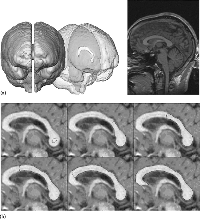
FIGURE 23.1
A corpus callosum (CC). (a) The CC is the band of nerve fiber tissue connecting the left and right hemispheres of the brain. (b) An energy minimization segmentation process. A shape model with progressively lower energy (left to right), showing a minimum of the energy function in bottom right. (Adapted from McIntosh, C. and Hamarneh, G., Vessel crawlers: 3D physically-based deformable organisms for vasculature segmentation and analysis, IEEE Computer Society Conference on Computer Vision and Pattern Recognition, 2006, Vol. 1, pp. 1084–1091, 2006a; Hamarneh, G. and McIntosh, C., Physically and statistically based deformable models for medical image analysis (Chapter 11), Deformable Models: Biomedical and Clinical Applications, pp. 335–386, 2007.)

23.1 Definitions and Foundations

We first give an outline of the energy minimization for MIS process. We define a medical image I_i and its corresponding segmentation (i.e., pixel labels) S_i, each having N pixels. Then I = {I₁, I₂,…, I_ℕ} and S = {S₁, S₂,…, S_ℕ} are sets of images and their corresponding ground-truth segmentations. In a slight abuse of the notation, we occasionally omit the subscript i from I_i and S_i for clarity and instead use I and S.

The first step in any energy minimization problem is the identification of the form of the energy function. In the next section, we will briefly group some popular energy terms into three main categories: boundary, region, and shape. Boundary terms are concerned primarily with the object boundary, region terms with the region inside or outside the object, and shape terms with the shape of the object. Other energy terms include spatial constraints on multipart objects, for example, containment (or layering), exclusion, or the number of labels (Delong et al., 2012; Nosrati and Hamarneh, 2013; Ulen et al., 2013; Yazdanpanah et al., 2011). Here we use these groupings to build a general energy functional. It may be convex or non-convex, as can the shape space over which it will be mini-mized. A general form is E(S, I, w) = w₁ × boundary(S, I) + w₂ × region(S, I) + w₃ × shape Prior(S), with free parameter w = [w₁, w₂, w₃]. Depending on the value of w, minima of E tend toward best satisfying the boundary, region, or shape terms. We note that the boundary and region terms are often referred to as external terms, since they involve cues external to the shape model, while the shape prior is deemed an internal term. More generally, we can write

E (S, I, w) = w_{1} J_{1} (S, I) + w_{2} J_{2} (S, I) + \dots + w_{n} J_{n} (S, I), (23.1)

$E (S, I, w) = w_{1} J_{1} (S, I) + w_{2} J_{2} (S, I) + \dots + w_{n} J_{n} (S, I), (23.1)$

where

J_i is the ith energy term

w = [w₁,…,w_n] are the weights

We note here that depending on the nature of S, E may be called an energy function or an energy functional, with the latter indicating S itself is a function.

The segmentation problem is to solve

S * = \underset{s}{\arg \min} E (S | I, w), (23.2)

$S * = \underset{s}{\arg \min} E (S | I, w), (23.2)$

which involves choosing a w and, depending on the nature of the energy functional, may also require training appearance and/or shape priors using I and/or S and setting an initialization. A gradient-descent-based solver is typically used but combinatorial approaches have also been explored for dis-cretized versions of the problem (Boykov and Kolmogorov, 2003) (see Section 23.5 for details). In either case, non-convexity, or supermodularity for combinatorial problems, can be quite problematic. There is no guarantee that another solution does not exist that better minimizes the energy and thus is potentially a better segmentation (Figure 23.2). Ideally both functional and shape spaces are convex, guaranteeing globally optimal solutions. However, whether convex or not the ground-truth segmentation, S_i, for image, I_i is not guaranteed to be an optima (local or global) of E(S|I_i, w). The goal, in general, is to build an E(S|I_i, w) such that S* is as close as possible to S_i under some definition of closeness [e.g., (Dice, 1945; Jaccard, 1901; Tanimoto, 1957)].

One of the earliest developed, and perhaps most recognized, examples of energy minimization methods being applied to image segmentation is that of deformable models. Deformable models for MIS gained popularity since the 1987 introduction of snakes by Terzopoulos et al. (Kass et al., 1987; Terzopoulos, 1987). At a high level, energy-minimizing deformable models work by deforming a user provided initial shape to fit to a target structure in a medical image. Shape-changing deformations result from the minimization, with respect to the shape, of a cost function measuring how plausible is the shape model and how well it aligns with the boundaries of the target anatomy in the image. Since the shape model itself is most commonly represented by a function, the cost function is often termed an energy functional and its gradient is derived using methods from variational calculus. The shape deformations are therefore typically simulated by solving an initial value problem using gradient-descent optimization algorithms (Elsgolc, 1962, G2). One further development, “Deformable organisms,” uses artificial life modeling techniques to augment the energy-minimizing deformable models with models of cognition, behav-iors, and sensory input (Hamarneh et al., 2001, 2009).

We now begin our more in-depth discussion of the different components of the energy minimization for MIS process.

23.1.1 Energy Function

Since snakes paved the way, there have been numerous papers attempting to increase accuracy by contributing novel energy terms, each designed to address a particular class of images or alleviate a particular problem with the original terms. As there have been far too many proposals to survey them all, here we focus on the key terms, many of which themselves have spawned numerous new approaches to MIS or changed the way we think about the problem at hand. As much of the initial development focused on external energy terms, namely, on the boundary and region terms that deal with the image processing itself, we begin our discussion there.

One of the most fundamental problems noted with snakes relates to their boundary capture range. If placed near a strong edge in an image, the contour would quickly snap to the edge, but if initialized farther away the influence of the edge would not reach the contour. There are, in fact, numerous causes of this problem relating to not only the external energy terms (Caselles et al., 1997; Cohen, 1991; Xu and Prince, 1998) but also the way the segmentation was originally represented (an explicit contour—see Section 23.1.2 for details) and the minimization technique being used.

Images

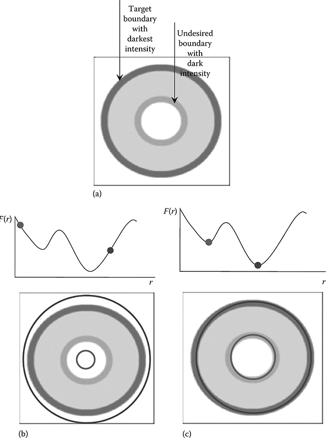
FIGURE 23.2
Synthetic example of single parameter deformable model with local minima. The circular deformable model's only parameter is its radius r. The energy function F(r) is minimal for the circle with darkest average intensity. The input image is shown in (a) with the darkest outmost boundary representing the global minima. In (b) two deformable models are initial-ized. In (c) after gradient descent, each model has moved to the nearest minima. (Reprinted from McIntosh, C., Energy functionals for medical image segmentation: Choices and consequences, PhD dissertation, Simon Fraser University, Burnaby, BC, Canada, Copyright 2011. With permission.)

An early attempt to rectify the aforementioned problem was by adding a deflation or inflation force to the contour that would attempt to shrink/grow it toward edges (Cohen, 1991). Rather than rely on a constant force, gradient vector flows extend the influence of edges off into homogeneous regions, thus increasing the capture range (Xu and Prince, 1998). Geodesic active contours (GACs) were similarly developed by both Caselles et al. (1997) and Yezzi et al. (1997). The approach of Caselles et al. formulated a deformable model optimization problem as that of finding the optimal path in a Riemannian space. Termed GACs, these popular deformable models work by minimizing curve length, where length is measured as the geodesic distance on a Riemannian manifold defined via an edge indicator function. The shortest curve is then, by definition, the curve along the edges of the image, and thus GACs automatically shrink the curve to the edges. GACs have become the canonical example of boundary-based deformable models.

However, what about objects whose boundaries blurred due to their inherent nature or noise, like the example in Figure 23.3? In these cases the intensity statistics of the areas both inside and outside the contour can be used to attempt to divide the image into maximally separated regions. The approaches of Chan et al. and of Yezzi et al. (Chan and Vese, 2001; Tsai et al., 2001) were similarly developed. Both are modeled after the Mumford–Shah functional wherein images are approximated by piecewise-smooth functions (Mumford and Shah, 1989). The approach of Chan and Vese is referred to as active contours without edges (ACWE) and has become a popular example of energy minimization for image segmentation. However, in their initial formulations, both methods approximate images by piecewise-constant functions, that is, objects are assumed to have a constant intensity. When objects are noisy, or their intensity changes gradually, a piecewise-smooth approximation is better suited, and thus an extension to piecewise-smooth functions was developed (Chan et al., 2007).

Images

FIGURE 23.3
An energy minimization segmentation process. A shape model with progressively lower energy (left to right), showing a minima of the energy function in bottom right. Notice the leaking into neighboring structures that occurs as a result of weak edge strength. (Reprinted from McIntosh, C. and Hamarneh, G., 2006b, Genetic algorithm driven statistically deformed models for medical image segmentation, ACM Workshop on Medical Applications of Genetic and Evolutionary Computation Workshop (MedGEC), in Conjunction with the Genetic and Evolutionary Computation Conference (GECCO), Seattle, WA, 2006b. With permission.)

When both boundary- and region-derived statistics are not enough, shape-based terms are used. Shape terms provide resilience to false boundaries by heavily penalizing the implausible shape configurations that the false boundaries imply. The most basic terms attempt to achieve boundary smoothness by minimizing curve length, segmentation area, or curvature. More advanced terms compare the shape of the segmentation to some prior model of the shape in an effort to minimize their dissimilarity (Cootes et al., 1992, 1995, 2001; Cootes and Taylor, 1997; Cremers et al., 2001, 2002, 2008; Dambreville et al., 2006; Etyngier et al., 2007; Leventon et al., 2000; Paragios et al., 2006; Pohl et al., 2007; Vu and Manjunath, 2008; Warfield et al., 2000) (see Section 23.1.4 for discussions).

There has even been work trying to combine edge terms, piecewise-constant terms, and shape terms into a single formulation (Bresson et al., 2006). However, with so many competing assumptions about the object and the image inherent in each formulation, some level of trade-off must be established in the resulting functional (i.e., the weights, w, must be set).

If not appropriately set, the weights w can cause significant error. In fact, our results demonstrated that optimizing the weights has dramatic effects, reducing error in large data sets by as much as 60% (McIntosh and Hamarneh, 2007). However, optimizing the weights by hand for even a single image can be a long and tedious task, with no real guarantee of obtaining the correct segmentation. As such, there has been a number of works that seek to automatically set the weights (Anguelov et al., 2005; Finley and Joachims, 2008; Kolmogorov et al., 2007; McIntosh and Hamarneh, 2007, 2009; Szummer et al., 2008; Taskar et al., 2005 Rao et al., 2009, 2010).

Instead of guessing the optimal weights, suppose we write a function γ(w|I_j, S_j) evaluating how well weight w works for a given image-segmentation pair (I_j, S_j), such that a parameter is deemed better when it causes S* to approach S_j, that is, the minimum of E to be the correct segmentation. Given S_j, we could then calculate the ideal weights for a particular image I_j by solving $w * = \underset{w}{\arg \min} γ (w | I_{j}, S_{j})$ $w * = \underset{w}{\arg \min} γ (w | I_{j}, S_{j})$ . It is important that γ itself be convex or globally solvable in w. If γ was not globally solvable, uncertainty would remain in that another w* may better minimize γ and thus better segmentthe image. Similarly, γ cannot contain free parameters, else those parameters would themselves introduce uncertainty, as was the case in McIntosh and Hamarneh (2007).

Recent advances in maximum margin estimation allow for weight opti-mization wherein the parameters of the objective function are sought such that the highest scoring structures (in our case segmentations) are as close as possible to the ground truth (Anguelov et al., 2005; Finley and Joachims, 2008; Szummer et al., 2008; Taskar et al., 2005). These methods do however assume that a single set of weights works for the entire test set of images, whereas different images can easily require different weights. In contrast, Kolmogorov et al. seek an optimal parameter on a per-image basis. Given a parameter range, their method simultaneously solves the objective function for a set of parameters that bound how the parameters influence the solution (Kolmogorov et al., 2007). Each solution is then treated as a potential segmentation. They propose a number of heuristics, including user intervention, to select the best segmentation from a set of potential ones.

A related topic is that of multiobjective optimization, where methods try to jointly minimize the terms, without weighting them. As the topic relates more to minimizing energy functionals, we defer its discussion until Section 23.1.5.

23.1.2 Segmentation Representation

As expected, all functions must have domains and so in turn energy functionals must have domains. That domain is the space of possible segmentations of the image or shapes. There are many different ways to represent the underlying segmentation, and that choice in turn impacts the image and shape terms that can be readily evaluated. For example, a shape using closed contours pairs most readily with region statistics. Here we summarize some of the most prevalent shape representations in use.

Naturally, we start with the representation originally detailed by Terzopolous et al., namely the explicit contour model (Kass et al., 1987; Terzopoulos, 1987). The contour is defined as an explicit, parameterized function of its arc length. Integrating along the arc-length integrates along the contour and allows for the evaluation of both internal and external terms (see Appendix B for details). These methods were extended to represent not only contours but surfaces and volumes (Cohen et al., 1992; Cohen and Cohen, 1993; Delingette et al. 1992; McInerney and Terzopoulos, 1995a; Miller et al., 1991; Staib and Duncan, 1992b; Whitaker, 1994). Other explicit models were introduced relating to spring-mass systems, where each boundary point is a mass, connected to other masses via springs (McInerney and Terzopoulos, 1996; Montagnat et al., 2001). There can be other types of masses, namely, internal nodes and medial nodes (Pizer et al., 2003). However, in general these aforementioned works are constrained to a fixed topology, which posed problems in many applications.

There have been two major directions of work to address topological adaptability. The first direction focused on novel ways to automatically re-parameterize the contour or surface enabling the evolution into complex geometries (McInerney and Terzopoulos, 1995b,c, 1999, 2000). Initially developed in 2D, T-snakes work by subdividing the image domain into a Freudenthal triangulation (McInerney and Terzopoulos, 1995b,c). At each deformation step, the intersections of the contours with the triangular grids are found, and a set of rules is followed to determine if the contour point should be split or merged. This work was later extended to 3D, with the introduction of T-surfaces (McInerney and Terzopoulos, 1999, 2000). Delingette simultaneously developed a somewhat related approach where simplex meshes are used to model the shape, and topological changes are performed “semi-automatically with an automatic detection of topological problems, but a manual validation of all operations” (Delingette, 1999). However, in both cases the explicit re-parameterization of the contour or surface can be costly and may not generalize well to even higher dimensions.

In contrast, implicit contours were built from the ground up to handle changes in topology (Caselles et al., 1997; Osher and Paragios, 2003; Osher and Sethian, 1988; Sethian, 1996). In these representations, the boundary is implied by a given function, instead of explicitly defined. Implicit representations are built around the signed distance function (SDF), where the object boundary is defined as the zero level set of the function. Integrating over the domain of the SDF implicitly integrates over the contour and thus allows for the evaluation of both internal and external terms, as before. Changes in topology are handled internally by the shape representation and require no re-parameterization of the model (Figure 23.4). Similarly, other functions can be used to implicitly represent shapes including characteristic functions (Tsai et al., 2004) and probability maps (Cremers et al., 2008).

More recently, graph methods have emerged where the segmentation is represented by the assignment of labels to a graph (Barrett and Mortensen, 1997; Boykov and Funka-Lea, 2006; Boykov and Jolly, 2001; Boykov and Kolmogorov, 2003; Falcão et al., 1998; Falcão and Udupa, 1997; Grady, 2006; Mortensen and Barrett, 1998; Shi and Malik, 2000). Pixels are represented as vertices in the graphs, and edges between pixel–vertices represent a connectivity neighborhood. Energy functionals, often called cost functions in graph-based works, are expressed as sums over the vertices and their neigh-borhoods that vary as a function of how each vertex is labeled.

Finally, our discussion thus far has been limited to that of a single object class, but it is also possible to represent multiple object classes at one time, using so-called multi-class shape representations that are built on both implicit (Paragios and Deriche, 2000, 2002; Samson et al., 2000; Vese and Chan, 2001; Zhao et al., 1996) and graph-based representations (Boykov and Jolly, 2001; Grady and Funka-Lea, 2004). Implicit shape models are adapted to multiple classes by defining multiple implicit functions, where the combinations and intersections of the functions denote which class is being represented. Graph methods, however, are extended by increasing the number of possible labels for each vertex.

Images

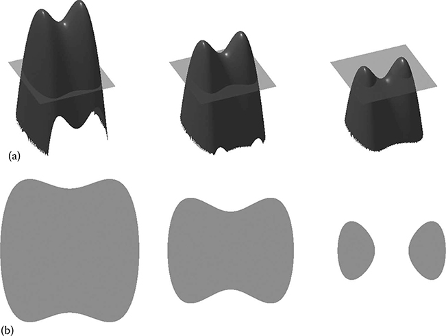
FIGURE 23.4
An exemplar SDF as a shape representation. (a) An SDF undergoing a simple deformation from left to right. (b) The zero level sets of the SDFs, displaying the segmentation each SDF represents. Notice how the topology automatically changes without any re-parameterization. (Reprinted from McIntosh, C., Energy functionals for medical image segmentation: Choices and consequences, PhD dissertation, Simon Fraser University, Burnaby, BC, Canada, Copyright 2011. With permission.)

In the end, the choice of representation is ultimately determined by the desired segmentation task. As such, it is worth noting that specialized models can exist, where a shape representation is designed specifically for one type of anatomy. A popular example is that of tubular-branching objects, namely, vessels, where cylindrical models can be built and deformed (McIntosh and Hamarneh, 2006; O'Donnell et al., 1994).

23.1.3 Image Representation

As might be expected, how the image is represented will impact how the terms of the energy functional can be evaluated on it. In fact, early on there were many contributions demonstrating how existing techniques could be modified to fit higher dimensional data, vector-valued data (Ballerini, 2001; Chan et al., 2000; Sapiro, 1996; Shah, 1996; Shi et al., 2008), tensor data (Nand et al., 2011; Rousson et al., 2004; Wang and Vemuri, 2004; Weldeselassie and Hamarneh, 2007) (Chapter 19), texture-heavy images (Paragios and Deriche, 2000, 2002), or even temporal data (Saad et al., 2008 Hamarneh et al., 2004; Tang et al., 2012; Rana et al., 2009; Ng et al., 2012), as opposed to the static, 2D, grayscale images early algorithms were presented on. Furthermore, numerous methods have been adapted to handle the intricacies of specific medical imaging modalities including magnetic resonance images and ultrasound. As an example, we talk briefly about some of the issues inherent to angiography in Section 23.2.

23.1.4 Training Data

A substantial amount of knowledge is often available about anatomical structures of interest—characteristic shape, position, orientation, symmetry, relationship to neighboring structures, associated landmarks, etc. and about plausible image intensity characteristics, subject to natural biological variability or the presence of pathology. Once collected, the training data typically come into the energy functional in the place of shape priors (Cootes et al., 1995), but appearance priors (Cootes et al., 2001) have also been developed (see Heimann and Meinzer (2009) for a complete survey). As shape priors have been a particular area of interest in the field, here we discuss some of the key works.

In many applications, prior knowledge about object shape variability is available or can be obtained by studying a training set of shape examples. This knowledge restricts the space of allowable deformations to a learned shape space that approximates the space of anatomically feasible shapes (Cootes and Taylor, 1997; Cootes et al., 1992, 1995, 2001; Cremers et al., 2001, 2002, 2008; Dambreville et al., 2006; Etyngier et al., 2007; Leventon et al., 2000; Paragios et al., 2006; Pohl et al., 2007; Vu and Manjunath, 2008; Warfield et al., 2000). One of the most notable works in this area is that of Cootes et al., where they introduced and refined active shape models (ASM) (Cootes et al., 1992, 1993, 1995). In ASM, principal component analysis (PCA) is calculated over a set of landmark points extracted from training shapes. The resulting principal components are used to construct a point distribution model (PDM) and an allowable shape domain (ASD). In a natural extension to their previous work, Cootes et al. modify their method to include image intensity statistics (Cootes et al., 2001). Staib and Duncan constrained the deformable models in Fourier space by conforming to probability distributions of the parameters of an elliptic Fourier decomposition of the boundary (Staib and Duncan, 1992a). Statistical prior shape knowledge was also incorporated in implicit, level set-based deformable models. Leventon et al. introduced statistical shape priors by using PCA to capture the main modes of variation of the level set representation (Leventon et al., 2000). However, as Pohl et al. point out, level sets do not form a vector space and hence more accurate shape statistics could be captured by transforming the shapes into a vector space using the logarithm of odds before performing PCA (Pohl et al., 2007).

Though simpler to optimize than their nonlinear counterparts, linear models of shape deformation may not always adequately represent the variance observed in real data. Linear shape models assume the data lies on a linear manifold, but shapes often lie on nonlinear manifolds where the manifold's properties are not accurately captured by linear statistics (Fletcher et al., 2004). For example, try fitting an ellipse to an “S”-like shape space. In order to include the entire letter, extraneous white space (nonvalid shapes) must also be included. Nonlinear shape models have been introduced to address this problem (Cootes and Taylor, 1997; Cremers, 2008; Cremers et al., 2001, 2002; Dambreville et al., 2006; Etyngier et al., 2007; Fletcher et al., 2004; Sozou et al., 1995).

However, we argue that the problem with linear statistics, as described earlier, is not necessarily due to the application of a linear model to nonlinear data but rather because of the implicit nature in which the statistics are applied (McIntosh and Hamarneh, 2011). By implicit we mean the statistics attempt to model variation in the shape, rather than variation in the parameters governing the deformations themselves. Note that we are not referring to the shape representation being implicit or explicit but instead whether the deformations are implicitly or explicitly studied. Implicit shape statistics result from the majority of previous deformable model approaches adopting a boundary-based shape representation, aside from a few exceptions (Pizer, 2003). As a consequence, the statistics are calculated using boundary models of the shape instead of models representing the interior and skeletal topology of the structures. Studying the underlying structural changes of a shape allows deformations that were previously non-convex to be decomposed into linear models. We refer to these as explicit shape statistics since they are calculated over the very parameters responsible for varying the object's shape. Consider an object represented by a single pixel. Different images of the object show the pixel moving around in a circle. A nonlinear function is required to describe the pixel's motion and hence no linear statistics can capture the motion adequately as long as it is the object's x, y position being studied. However, once decomposed into a function of sin and cos, the underlying parameter that controls the objects variability is linear in its variation, and hence linear statistics will yield greatly improved shape statistics. The same argument carries forward, albeit more complexly, to a more complex object. A simple bending of a shape's medial axis is a linear deformation under the appropriate representation, as it is simply a rotation of some of the medial nodes. However, the bending is a highly non-convex deformation once embedded in the image domain, as either an implicit shape (Pohl et al., 2007) or an explicit boundary-based model (Cootes et al., 1995).

23.1.5 Minimizer

Once the image and shape representations have been set and the problem formulated, all that is left is to solve the minimization process and obtain the resulting segmentation. Though it may sound simple enough, this area has been a major focus of criticism of energy minimization-based methods over the years, and as such has recently become one of the most focused areas for research. Specifically, in their original inception, many of the aforementioned methods were plagued by problems of local minima and sensitivity to initialization. Here we describe the changes and revelations in the field on this topic over the past decade. For a broader review, the interested reader is referred to the following representative, but far from comprehensive, list: Cremers et al., 2011; Grady and Polimeni, 2010; Kolmogorov and Zabin, 2004; and Nikolova et al., 2006.

Energy functional minimization can be carried out in a variety of ways. One solution is to perform explicit differentiation under the Euler–Lagrange equations, where each new application with a modified energy functional must be accompanied by one such derivation (Caselles et al., 1997; Chan and Vese, 2001; Kass et al., 1987; Terzopoulos, 1987) (see Appendix A for details). The result is a set of equations, which, if satisfied, guarantee a stationary point of the energy functional. The solution is then obtained through a gradient-descent process where the change in the shape model (with respect to an artificial time variable) is equated to the Euler–Lagrange equation, that is, the deformable models come to rest when the equations are satisfied (Kass et al., 1987; Terzopoulos, 1987). There are, however, two main drawbacks with this approach. Firstly, performing gradient descent in the presence of image noise can lead to instability in the deformations over time (Sundaramoorthi et al., 2007). Secondly, as the number of dependent variables (shape, location, scale, orientation, etc.) increases so does the complexity of the search space, which often increases the number of local min-ima and requires the calculation of an increasingly large number of derivatives.

On the issue of stability, there has been work by Sundaramoorthi et al. on reformulating the gradient flow using Sobolev-type inner products, which induce favorable regularity prosperities into the flow, thus bringing smoother deformations over time (Sundaramoorthi et al., 2007). Recently Bar and Sapiro introduced a Newton-type method built on more general-ized norms than the L² norm, obtained by equating the Euler–Lagrange constraint to an artificial time variable (Bar and Sapiro, 2009). They include the Sobolev norm and demonstrate improved results over L² norms, with faster convergence and more accuracy in the presence of noise. Unless used on convex problems, however, these methods are still prone to local minima.

If local minima do not suffice, global minima must be sought, and as such there have been a number of recent approaches to obtaining the global optima of energy functionals (Andrews et al., 2011b; Appleton and Talbot, 2006; Barrett and Mortensen, 1997; Boykov and Funka-Lea, 2006; Boykov and Kolmogorov, 2003; Bresson et al., 2007; Cremers et al., 2008; Falcão and Udupa, 1997; Falcão et al., 1998; Grady, 2006; Li and Yezzi, 2006; Mortensen and Barrett, 1998; Nikolova et al., 2006). There are three primary directions toward this goal: min-paths, min-cuts, and convex approximations.

Min-path techniques are formulated on the basis of Dijkstra's algorithm for finding the shortest path in an undirected graph with nonnegative edge weights. They were first presented for 2D interactive segmentation (Barrett and Mortensen, 1997; Falcão and Udupa, 1997), extended to 3D (Falcão and Udupa, 1997), and later specialized to 4D for vessel segmentation (Li and Yezzi, 2006; Poon et al., 2008, kawahara et al., 2013, Wink et al., 2004) and 6D (or higher) for spinal cord segmentation (Kawahara et al., 2013).

Graph cuts were demonstrated as a global minimization technique for a popular energy functional (Caselles et al., 1997), as a special case of computing a geodesic on a Riemannian space whose metric is computed from the image (Boykov and Kolmogorov, 2003). However, graph cuts have been shown to apply only to a restricted class of energy functionals that are submodular (Kolmogorov and Zabin, 2004), and their solutions are discrete approximations to the continuous formulations whose accuracy is dependent on the resolution of the approximating graph (Boykov and Kolmogorov, 2003). Naturally, as that resolution increases so does their running time. Random walkers were developed in a similar nature, solving image segmentation as a graph problem wherein the global optimum is obtained to a particular cost function (Grady, 2006). In fact, graph cuts and random walkers have been shown to be specific instantiations of a single framework (Sinop and Grady, 2007).

Another line of work has come from the relaxation of the underlying shape model from a non-convex space to a convex one, thereby defining convex energy functionals that can then be minimized instead of their non-convex counterparts. This convex relaxation work, which began in 2004 with a simple restricted class of functionals (Nikolova et al., 2006), was later extended to a broader class in Bresson et al. (2007), and then a similar work appeared in 2008 with the addition of a shape prior (Cremers et al., 2008). However, restrictions still exist in that the functionals and the shape spaces they are optimized over must be convex when defined over the relaxed space and that the relaxed shape space must itself be convex.

Though not guaranteed to find global optima, genetic algorithms (GAs) have also been applied to the minimization of energy functionals (Ballerini, 1998, 2001; Fan et al., 2002; Ibáñez et al., 2009; MacEachern and Manku, 1998; McIntosh and Hamarneh, 2011; Tohka, 2001). At a high level, GAs work by performing many simultaneous local searches, each individually optimizing the energy functional via a random walk in the search space. At the end of the process, the search that yielded the lowest value for the energy functional is adopted as the segmentation.

Ballerini extends the classical active contour models, developed by Terzopoulos (1987), by using GA to directly minimize the standard energy functional (Ballerini, 1998). Members of the GA population are hypothetical shape configurations, represented by their explicit contour locations. The method was later extended to color images by using one image term per color channel (Ballerini, 2001). MacEachern and Manku presented a similar method using a binary representation of the contour (MacEachern and Manku, 1998). Similarly, Tohka presented simplex meshes paired with image-based energies, minimized via a hybrid GA-greedy approach, and applied the technique to the segmentation of 3D medical images (Tohka, 2001). Fan et al. also developed a GA method for an explicit active contour but describe their method using Fourier descriptors and employ parallel GAs to speed up minimization (Fan et al., 2002). A different shape representation, known as topological active nets, is used by Ibáñez et al. to enable the segmentation of objects with unknown topologies or even multiple objects in the same scene (Ibáñez et al., 2009). However, aside from simple boundary smoothness constraints, all of these methods are based on classical active contour models or their variants without incorporating prior shape knowledge, making them prone to latching to erroneous edges and ill-equipped to handle gaps in object boundaries (as was discussed in Section 23.1.1).

In Hill and Taylor (1992), GAs were used with statistically based ASMs, where the parameter space consists of possible ranges of values for the pose and shape parameters of the model. The objective function to be maximized reflects the similarity between the gray levels related to the object in the search stage and those found from training. Additional works use convex, implicit, global shape statistics assuming a Gaussian distribution around a mean shape (Ghosh and Mitchell, 2006; Mignotte and Meunier, 1999; Ruff et al., 1999). Mignotte and Meunier (1999) incorporate prior shape information by defining the mean as a circular deformable template, while Ruff et al. (1999) use a PDM for occluded shape reconstruction, and Ghosh and Mitchell (2006) use a level set shape representation and a learned mean from training data. Although these techniques apply GAs to produce generations of plausible populations of shapes, the statistically based deformations are convex and may not offer the required flexibility to accommodate for nonlinear shape deformations. In McIntosh and Hamarneh (2011), we address this problem by using GAs to optimize statically based deformations that explicitly study the underlying shape variations, thus reducing the problem with linear shape statistics described in Section 23.1.4.

A somewhat related direction is that of multiobjective optimization, where each term is simultaneously optimized rather than optimizing a linear sum of the terms (23.1). Hence, in multiobjective optimization no weights are provided to combine the competing terms of the functional, instead a solution is sought for which no term can be improved without sacrificing another (Collette and Siarry, 2002). That solution is known as a Pareto optimal solution (Collette and Siarry, 2002). The set of Pareto optimal solutions for a given problem is known as the Pareto front, and there is no preference among them unless a ranking is provided between the objectives. Nakib et al. recently used multiobjective optimization to determine the parameters for a thresholding algorithm for image segmentation (Nakib et al., 2010). Hanning et al. present an approach using a piecewise approximation of the image similar to the Mumford–Shah model (Mumford and Shah, 1989) using multiobjective optimization to decide the trade-off between the number of segments and the image approximation error (Hanning et al., 2006). It is interesting to note that, for convex functions, if the ground truth lies on the Pareto front, then by definition a set of weights must exist that causes the optima to be the ground truth for the linear sum of terms formulation (23.1) (Geoffrion, 1968). In other words, a linear sum of terms model exists that yields the same segmentation as the multiobjective model, which is far more challenging to optimize. However, the necessary weights needed to achieve the desired segmentation are unknown. Weight optimization attempts to determine these weights (Section 23.1.1).

23.1.6 Related Methods

Though our discussion thus far has been focused on energy minimization methods for image segmentation that follow the prescribed building blocks, there are a few bodies of related research that follow a different path. Here we briefly detail two of them.

23.1.6.1 Relation to Bayesian Methods

Throughout this chapter, we have examined numerous methods built on energy functionals of the form E(S|I,w) = w₁ × internal(S) + w₂ × external(S,I). However, an interesting parallel to probabilistic approaches can be observed with a few simple assumptions and manipulations of this general form. Here we demonstrate that this model is actually equivalent to performing image segmentation via Bayesian inference. First, we restate the segmentation problem as

S * = \underset{S}{\arg \max} P (S | I, w), (23.3)

$S * = \underset{S}{\arg \max} P (S | I, w), (23.3)$

where

P (S | I, w) = \frac{P (I | S, w) P (S | w)}{P (I | w)} . (23.4)

$P (S | I, w) = \frac{P (I | S, w) P (S | w)}{P (I | w)} . (23.4)$

Maximizing (23.3) is equivalent to minimizing its negative logarithm

S * = \underset{S}{\arg \min} (- \log P (S | I, w)), (23.5)

$S * = \underset{S}{\arg \min} (- \log P (S | I, w)), (23.5)$

where = −log P(I|S, w) − log P(S|w), and the denominator has been removed as it has no consequence on the minimization. Now suppose we model our probabilities as

\begin{array}{l} P (S | w) = e^{- w_{1} \times int e r n a l (S)} \\ P (S | I, w) = e^{- w_{2} \times e x t e r n a l (S, I)} \end{array} (23.6)

$\begin{array}{l} P (S | w) = e^{- w_{1} \times int e r n a l (S)} \\ P (S | I, w) = e^{- w_{2} \times e x t e r n a l (S, I)} \end{array} (23.6)$

then substituting back into (23.5) yields

S * = \underset{S}{\arg \min} (- \log P (S | I, w)) = w_{1} \times int e r n a l (S) + w_{2} \times e x t e r n a l (S, I), (23.7)

$S * = \underset{S}{\arg \min} (- \log P (S | I, w)) = w_{1} \times int e r n a l (S) + w_{2} \times e x t e r n a l (S, I), (23.7)$

as before. From here it becomes possible to examine many of the approaches previously cited and see what independence assumptions they are making from a Bayesian standpoint.

23.1.6.2 Relation to Segmentation via Registration

Thus far we have discussed methods where the dependent function of the energy functional is one describing the shape of the current segmentation. However, a related field exists where the dependent function is instead a spatial transformation describing how one or more images are related. This is the field known as image registration, and it involves finding a mapping from the spatial coordinates of one image to another, identifying which pixels in a source image map to which pixels in a target image. Image registration can be used for segmentation when the mapping from a novel image is found to a training image with a known segmentation, since that mapping effectively labels the novel image. As this field is far too large and diverse to cover here, we refer the interested reader to Maintz and Viergever (1998), Zitová and Flusser (2003), and Chapter 22, for a complete survey. We do note, however, that many of the same issues discussed in this chapter, that is, global versus local optima and setting the weights for the energy functional, are also important problems in registration.

23.2 MIS via Energy Minimization

As already noted in this chapter, energy minimization methods have been applied to a wide variety of MIS problems. Two popular application domains are those of cardiac images and vascular images. As an example of how energy minimization can be applied to MIS, here we briefly discuss some key works relating to vascular segmentation. Though a complete survey of energy mini-mization for MIS does not exist, the interested reader is referred to McInerney and Terzopoulos (1996) for a related survey of MIS using deformable models.

One structure of particular interest in the diagnosis and understanding of many diseases is vasculature (Bullitt et al., 2003). Vessel segmentation remains an interesting application area of energy minimization methods because of its unique challenges. Firstly, the topology is complex, and as such many of the already mentioned topology-adaptive shape models were first demonstrated in their application to vessel segmentation (McInerney and Terzopoulos, 2000). Secondly, the vessels are often of very low contrast motivating advances in image terms (Frangi et al., 1999; Vasilevskiy and Siddiqi, 2002; Wink et al., 2001, 2004). For example, Vasilevskiy and Siddiqi built flux-maximizing geometric flows based on the observation that the gradient vector field near a vessel should be orthogonal to the vessel (Vasilevskiy and Siddiqi, 2002). They define a flux-maximizing geometric flow as one for which the inward normals of the underlying curve align with the direction of the gradient vector field. Near vessels the gradient vector field points inward toward the vessel centerline, and thus maximizing the flux will align the boundary of the segmentation to the boundary of the vessel. The last major challenge in vessel segmentation is that the vessels can be very thin, pushing the boundaries of numerical stability in many techniques and motivating new methods with increased stability to thin structures (Lorigo et al., 2001; Sundaramoorthi et al., 2007). For example, Lorigo et al. modify GAC to deform along the medial axis of a tubular shape, as opposed to its surface (Lorigo et al., 2001). For a complete survey of vessel segmentation techniques, the reader is referred to Lesage et al. (2009).

23.3 Discussion

Having briefly touched on each of the five primary building blocks of energy minimization methods, we conclude with a discussion of the main issues concerning their usage for MIS, namely, issues relating to how to build the energy functional, represent the segmentation, deal with the different imaging modalities themselves, train priors, and finally minimize the resulting system. We begin by touching briefly on issues relating to validating the method, as that is a fundamental step that we have not yet discussed.

Every MIS method must be validated. There are two main approaches to validate an MIS method, expert segmentations and synthetic data, each of which has its own inherit advantages and drawbacks. Expert segmentations can be time consuming and costly to obtain. Furthermore, expert segmentations suffer from both inter- and intraoperator variability because multiple experts, or even the same expert on different days, can obtain differing segmentations of the same object. Warfield et al. attempt to address problems with inter- and intraoperator variability through an expectation–maximization algorithm that weights different segmentations according to a variety of measurements and rules (Warfield et al., 2004). The key advantage to expert segmentations of real medical data is that the data is real and hence it demonstrates the applicability of the method to the problem at hand. Synthetic data can be created by either physical or computational phantoms. Physical phantoms are those physically constructed and then imaged in some manner, whereas computational phantoms are simulated using mathematical models designed to replicate human anatomy under specific imaging protocols (Cocosco et al., 1997; Hamarneh and Jassi, 2010). The main drawback in both cases is realism: segmenting a phantom well does not necessarily mean real data will also be segmented with high accuracy. The main advantage of synthetic data is certainty about the ground-truth segmentations. In Hamarneh et al. (2008), a hybrid method based on synthesizing deformation of a real data is presented. Whether real data or synthetic data, a measure of dissimilarity between the automatic segmentation and the ground truth must eventually be computed. Standard approaches for evaluating segmentation results given ground-truth segmentation include the Hausdorff distance, the Dice similarity coefficient (Dice, 1945), the Jaccard index (Jaccard, 1901), and the Tanimoto coefficient (Tanimoto, 1957).

Choosing the right energy functional for the given task is a crucial first step. Ideally, one hopes for strictly convex functions with their global minima lying at the correct segmentations for a given set of images, but this ideal scenario is rarely the case. The main challenges here are determining what energy terms could make a good functional and how to weight them in a such way as to best segment the images, In other words, one must appreciate the trade-off between the fidelity of the energy functional (how accurately it models the segmentation problems at hand) and its optimizability (how attainable is the functional's global optimum) (Hamarneh et al., 2011; Ulen et al., 2013).

There are often two main concerns when choosing the segmentation representation. Firstly, will it allow for the training of appropriate shape priors? Secondly, will it introduce problems in the minimization stage? Some shape representations do not form vector spaces, and thus performing statistics on them is difficult. Level sets (SDFs) are one such example, where a specific method for computing statistics over the resulting shape space was needed (Pohl et al., 2007). Level set-based representations can also cause problems in the minimization stage, as they do not form a convex space, and thus introduced non-convexity into the minimization problem (Cremers et al., 2008). However, they remain a popular technique due to the sub-pixel accuracy and automatic handling of topological changes. A more recent representation is the isometric log ratio (Changizi and Hamarneh, 2010) that has been used for segmentation of anatomical images (Andrews et al., 2011a,b).

Each imaging modality has its own inherent problem associated with it relating to different types of noise and spatial or temporal resolution of the structure of interest. As already exemplified with a brief treatment of blood vessel segmentation methods, each application can require customized energy functionals, segmentation representations, and optimization strategies.

When training priors, one is often forced to balance two competing goals: having the priors accurate versus having the resulting energy functional solvable. Linear statistics do not often fit the training data well but lead to easily solved energy functionals, whereas nonlinear statistics fit the data but are difficult to work with. The problem with linear statistics, however, is often not necessarily due to the application of a linear model to nonlinear data but rather due to the global aspect of the shape statistics themselves and due to the shape representation to which they are applied. Global shape statistics are those that model the shape variation of the entire shape simultaneously, that is, each shape is a single point in some high-dimensional space and the statistics (linear or not) describe some restricted set of that space. Many deformable model approaches adopt a boundary-based representation. As a consequence the statistics are calculated using boundary models of the shape instead of models representing the interior and skeletal topology of the structures, leading to a loss of accuracy (McIntosh and Hamarneh, 2011).

The primary problem in minimization remains how to globally optimize an increasingly large set of energy functionals, as opposed to the restricted sets seen thus far (Bresson et al., 2007; Cremers et al., 2008; Kolmogorov and Zabin, 2004). Interestingly enough, even with global minima, existing functionals are not proving accurate enough, motivating the search for new energy terms or ways of building functionals that can better respect the image variability.

In short, developing MIS methods remains a daunting task from start to finish with numerous areas for research relating to each of the five building blocks commonly found in energy minimization techniques. However, with the ever-growing popularity of medical imaging for diagnosis and disease understanding, developing robust and automatic techniques for MIS remains an important goal. In order to reach that goal, we must continue to make breakthroughs in terms of accuracy and reliability of MIS methods. To do that, we need to consider where the bulk of the error and performance variability is coming from, so as to best focus our efforts there.

With fully automatic segmentation remaining an unsolved problem, user-based inspection and delineation of medical images is indispensable. This is trivial for scalar fields, but for complex manifold-valued images, even displaying these images requires careful considerations.

Realizing the challenge in achieving accurate yet fully automatic segmentation methods, recent methods opted to calculate the uncertainty in a resulting segmentation (e.g., via Shannon's entropy of probabilistic segmentation) and utilizing the uncertainty measures in active- and self-learning strategies (Andrews et al., 2011a,b; Changizi and Hamarneh; 2010, Saad et al., 2010a,b; Top et al., 2010, 2011).

Appendix 23.A Euler–Lagrange

Starting with a function Φ(x), we build an energy functional

E (Φ) = \int L (x, Φ (x), Φ_{x} (x), Φ_{x x} (x)) d x (23.A.1)

$E (Φ) = \int L (x, Φ (x), Φ_{x} (x), Φ_{x x} (x)) d x (23.A.1)$

where Φ_x is the first derivative of Φ with respect to x and Φ_xx the second. The functional E describes a desirable feature of Φ, in that it takes a high value when Φ is doing poorly and a low value when Φ is doing well. We know from Fermat's theorem that E obtains its extremum at a stationary point, that is, where the derivative is zero. To describe a stationary point one typically writes

\lim_{τ \to 0} \frac{E (Φ + τ ω) - E (Φ)}{τ} = 0 (23.A.2)

$\lim_{τ \to 0} \frac{E (Φ + τ ω) - E (Φ)}{τ} = 0 (23.A.2)$

where ω is a scalar, but here ω is a function, so this equation is known as the first variation, as opposed to fist derivative, of the functional. Developed in the 1750s, the Euler–Lagrange equation plays a fundamental role in variational calculus, defining a necessary condition under which the first variation tends to zero, and therefore the functional reaches a stationary point (Elsgolc, 1962). For a functional E as described earlier, the general form of the Euler–Lagrange differential equation is

\frac{\partial L}{\partial Φ} - \frac{\partial}{\partial x} (\frac{\partial L}{\partial Φ_{x}}) + \frac{\partial}{\partial x^{2}} (\frac{\partial L}{\partial Φ_{x x}}) = 0 (23.A.3)

$\frac{\partial L}{\partial Φ} - \frac{\partial}{\partial x} (\frac{\partial L}{\partial Φ_{x}}) + \frac{\partial}{\partial x^{2}} (\frac{\partial L}{\partial Φ_{x x}}) = 0 (23.A.3)$

See Appendix B for an example of its application to energy minimization methods for MIS.

Appendix 23.B Snakes: Details and Derivations

Classical deformable shape models (Terzopoulos, 1987) are represented as a 2D parametric contour v(s) = (x(s), y(s)), where s ∊ [0,1] traverses the contour (Figure 23.B.1) and v is deformed to fit to image data by minimizing an energy term ξ

ξ (v (s)) = α (v (s)) + β (v (s)), (23.B.1)

$ξ (v (s)) = α (v (s)) + β (v (s)), (23.B.1)$

which depends on both the shape of the contour and the image data I(x, y) reflected via the internal and external energy terms, α(v(s)) and β(v(s)), respectively.

The internal energy term is given as

α (v (s)) = {\int^{​}}_{0}^{1} \frac{1}{2} (w_{1} ‖ v_{s} ‖^{2} + w_{2} ‖ v_{s s} ‖^{2}) d s, (23.B.2)

$α (v (s)) = {\int^{}}_{0}^{1} \frac{1}{2} (w_{1} ‖ v_{s} ‖^{2} + w_{2} ‖ v_{s s} ‖^{2}) d s, (23.B.2)$

Images

FIGURE 23.B.2 A parameterized contour undergoing a simple deformation (left to right). (Reprinted from McIntosh, C., Energy functionals for medical image segmentation: Choices and consequences, PhD dissertation, Simon Fraser University, Burnaby, BC, Canada, Copyright 2011. With permission.)

whereas the external energy term is given as

β (v (s)) = {\int^{​}}_{0}^{1} w_{3} (s) P (v (s)) d s . (23.B.3)

$β (v (s)) = {\int^{}}_{0}^{1} w_{3} (s) P (v (s)) d s . (23.B.3)$

The weighting functions w₁ and w₂ control the tension and flexibility of the contour, respectively, and w₃ controls the influence of image data. w_i’s can depend on s but are typically set to different constants. For the contour to be attracted to image features, the function P(v(s)) is designed such that it has minima where the features have maxima. For example, for the contour to be attracted to high-intensity changes (high gradients), we can choose

P (v (s)) = P (x (s), y (s)) = - ‖ \nabla [G_{σ} * I (x (s), y (s))] ‖ (23.B.4)

$P (v (s)) = P (x (s), y (s)) = - ‖ \nabla [G_{σ} * I (x (s), y (s))] ‖ (23.B.4)$

where G_σ _* I denotes the image convolved with a smoothing (e.g., Gaussian) filter with a parameter σ controlling the extent of the smoothing (e.g., variance of Gaussian).

The contour v that minimizes the energy ξ must, according to the calculus of variations (Elsgolc, 1962), satisfy the vector-valued partial differential (Euler–Lagrange) equation

\frac{\partial f}{\partial v} - \frac{\partial}{\partial s} (\frac{\partial f}{\partial v_{s}}) + \frac{\partial^{2}}{\partial s^{2}} (\frac{\partial f}{\partial v_{s s}}) = 0 (23.B.5)

$\frac{\partial f}{\partial v} - \frac{\partial}{\partial s} (\frac{\partial f}{\partial v_{s}}) + \frac{\partial^{2}}{\partial s^{2}} (\frac{\partial f}{\partial v_{s s}}) = 0 (23.B.5)$

where $f = \frac{1}{2} (w_{1} {‖ v_{s} ‖}^{2} + w_{2} {‖ v_{s s} ‖}^{2}) - w_{3} ‖ \nabla (G_{σ} * I (v)) ‖$ $f = \frac{1}{2} (w_{1} {‖ v_{s} ‖}^{2} + w_{2} {‖ v_{s s} ‖}^{2}) - w_{3} ‖ \nabla (G_{σ} * I (v)) ‖$ . The first step in applying the Euler–Lagrange is to determine the partial derivatives as follows:

\begin{array}{l} \frac{\partial f}{\partial v} = - w_{3} \nabla ‖ \nabla (G_{σ} * I (v)) ‖ \\ \frac{\partial}{\partial s} (\frac{\partial f}{\partial v_{s}}) = w_{1} v_{s s} \\ \frac{\partial^{2}}{\partial s^{2}} (\frac{\partial f}{\partial v_{s s}}) = w_{2} v_{s s s s} \end{array} (23.B.6)

$\begin{array}{l} \frac{\partial f}{\partial v} = - w_{3} \nabla ‖ \nabla (G_{σ} * I (v)) ‖ \\ \frac{\partial}{\partial s} (\frac{\partial f}{\partial v_{s}}) = w_{1} v_{s s} \\ \frac{\partial^{2}}{\partial s^{2}} (\frac{\partial f}{\partial v_{s s}}) = w_{2} v_{s s s s} \end{array} (23.B.6)$

Then substituting back into Equation 23.B.5, we get the final set of equations

- w_{1} v_{s s} + w_{2} v_{s s s s} - w_{3} \nabla ‖ \nabla (G_{σ} * I ‖ = 0 (23.B.7)

$- w_{1} v_{s s} + w_{2} v_{s s s s} - w_{3} \nabla ‖ \nabla (G_{σ} * I ‖ = 0 (23.B.7)$

where we make note that v(s) = (x(s), y(s)), and so the earlier equation can be expanded to

\begin{array}{l} - w_{1} x_{s s} + w_{2} x_{s s s s} - w_{3} \frac{\partial ‖ \nabla (G_{σ} * I) ‖}{\partial x} = 0 \\ - w_{1} y_{s s} + w_{2} y_{s s s s} - w_{3} \frac{\partial ‖ \nabla (G_{σ} * I) ‖}{\partial y} = 0 \end{array} (23.B.8)

$\begin{array}{l} - w_{1} x_{s s} + w_{2} x_{s s s s} - w_{3} \frac{\partial ‖ \nabla (G_{σ} * I) ‖}{\partial x} = 0 \\ - w_{1} y_{s s} + w_{2} y_{s s s s} - w_{3} \frac{\partial ‖ \nabla (G_{σ} * I) ‖}{\partial y} = 0 \end{array} (23.B.8)$

In order to solve the system of equations, we introduce an artificial time step, by equating the earlier equations to −∂v/∂t. This yields a first-order iterative optimization method, though as outlined in this report other choices for optimization methods exist.

References

Andrews S., Hamarneh G., Yazdanpanah A., HajGhanbari B., and Reid D., 2011a, Probabilistic multi-shape segmentation of knee extensor and flexor muscles, in Lecture Notes in Computer Science, Medical Image Computing and Computer-Assisted Intervention (MICCAI), Vol. 6893, pp. 651–658.

Andrews S., Hamarneh G., Yazdanpanah A., HajGhanbari B., and Reid W.D., 2011a, Probabilistic multi-shape segmentation of knee extensor and flexor muscles, Lecture Notes in Computer Science, Medical Image Computing and Computer-Assisted Intervention (MICCAI), pp. 651–658.

Andrews S., McIntosh C., and Hamarneh G., 2011b, Convex multi-region probabilistic segmentation with shape prior in the isometric log-ratio transformation space, IEEE International Conference on Computer Vision (IEEE ICCV), Barcelona, Spain.

Andrews S., McIntosh C., and Hamarneh G., 2011b, Convex multi-region probabilistic segmentation with shape prior in the isometric Logratio transformation space, in IEEE International Conference on Computer Vision (IEEE ICCV), pp. 2096–2103.

Anguelov D., Taskarf B., Chatalbashev V., Koller D., Gupta D., Heitz G., and Ng A., 2005, Discriminative learning of Markov random fields for segmentation of 3D scan data, IEEE Computer Society Conference on Computer Vision and Pattern Recognition, 2005, CVPR 2005, Vol. 2, pp. 169–176, San Diego, CA.

Appleton B. and Talbot H., 2006, Globally minimal surfaces by continuous maximal flows, IEEE Transactions on Pattern Analysis and Machine Intelligence 28, 106–118.

Ballerini L., 1998, Genetic snakes for medical image segmentation, Proceedings of the SPIE Conference on Mathematical Modeling and Estimation Techniques in Computer Vision, Vol. 3457, pp. 284–295, San Diego, CA.

Ballerini L., 2001, Genetic snakes for color images segmentation, in Applications of Evolutionary Computing (ed. Boers E.), Vol. 2037 of Lecture notes in Computer Science, Springer, Berlin/Heidelberg, Germany, pp. 268–277.

Bar L. and Sapiro G., 2009, Generalized Newton-type methods for energy formulations in image processing, SIAM Journal of Imaging Science 2(2), 508–531.

Barrett W.A. and Mortensen E.N., 1997, Interactive live-wire boundary extraction, Medical Image Analysis 1(4), 331–341.

Boykov Y. and Funka-Lea G., 2006, Graph cuts and efficient N-D image segmentation, International Journal of Computer Vision (IJCV) 70(2), 109–131.

Boykov Y. and Jolly M.P., 2001, Interactive graph cuts for optimal boundary & region segmentation of objects in n-d images, Proceedings of the Eighth IEEE International Conference on Computer Vision, 2001, ICCV 2001, Vol. 1, pp. 105–112, Vancouver, BC, Canada.

Boykov Y. and Kolmogorov V., 2003, Computing geodesics and minimal surfaces via graph cuts, Proceedings of the Ninth IEEE International Conference on Computer Vision, 2003, Vol. 1, pp. 26–33, Nice, France.

Bresson X., Esedoḡlu S., Vandergheynst P., Thiran J.P., and Osher S., 2007, Fast global minimization of the active contour/snake model, Journal of Mathematical Imaging and Vision 28(2), 151–167.

Bresson X., Vandergheynst P., and Thiran J.P., 2006, A variational model for object segmentation using boundary information and shape prior driven by the Mumford-Shah functional, International Journal of Computer Vision 68(2), 145–162.

Bullitt E., Gerig G., Aylward S., Joshi S., Smith K., Ewend M., and Lin W., 2003, Vascular attributes and malignant brain tumors, Medical Image Computing and Computer-Assisted Intervention—MICCAI 2003, Vol. 2878 of Lecture notes in Computer Science, Springer, Berlin/Heidelberg, Germany, pp. 671–679.

Caselles V., Kimmel R., and Sapiro G., 1997, Geodesic active contours, International Journal of Computer Vision 22, 61–79.

Changizi N. and Hamarneh G., 2010, Probabilistic multi-shape representation using an isometric log-ratio mapping, in Lecture Notes in Computer Science, Medical Image Computing and Computer-Assisted Intervention (MICCAI), Vol. 6363, pp. 563–570.

Changizi N. and Hamarneh G., 2010, Probabilistic multi-shape representation using an isometric log-ratio mapping, Lecture Notes in Computer Science, Medical Image Computing and Computer-Assisted Intervention (MICCAI), pp. Part III: 563–570.

Chan T., Moelich M., and Sandberg B., 2007, Some recent developments in variational image segmentation, Image Processing Based on Partial Differential Equations, Springer, Berlin, Germany, pp. 175–210.

Chan T. and Vese L., 2001, Active contours without edges, IEEE Transactions on Image Processing 10(2), 266–277.

Chan T.F., Sandberg B.Y., and Vese L.A., 2000, Active contours without edges for vector-valued images, Journal of Visual Communication and Image Representation 11(2), 130–141.

Cocosco C.A., Kollokian V., Kwan R.K.S., Pike G.B., and Evans A.C., 1997, Brainweb: Online interface to a 3D MRI simulated brain database, NeuroImage 5, 425.

Cohen I., Cohen L., and Ayache N., 1992, Using deformable surfaces to segment 3-d images and infer differential structures, CVGIP 56(2), 242–263.

Cohen L. and Cohen I., 1993, Finite-element methods for active contour models and balloons for 2-d and 3-d images, IEEE Transactions on Pattern Analysis and Machine Intelligence 15(11), 1131–1147.

Cohen L.D., 1991, On active contour models and balloons, Computer Vision Graphics and Image Processing: Image Understanding 53(2), 211–218.

Collette Y. and Siarry P., 2002, Multiobjective Optimization Principles and Case Studies, Decision engineering, Springer, Berlin, Germany.

Cootes T., Taylor C., Cooper D., and Graham J., 1992, Training models of shape from sets of examples, British Machine Vision Conference, pp. 9–18. Springer-Verlag, Leeds, UK.

Cootes T., Taylor C., Hill A., and Halsam J., 1993, The use of active shape models for locating structures in medical images, Proceedings of the 13th International Conference on Information Processing in Medical Imaging, Flagstaff, AZ, pp. 33–47. Springer-Verlag.

Cootes T. and Taylor C., 1997, A mixture model for representing shape variation, British Machine Vision Conference, pp. 110–119. Springer-Verlag, University of Essex, UK.

Cootes T.F., Cooper D., Taylor C.J., and Graham J., 1995, Active shape models—their training and application, Computer Vision and Image Understanding 61, 38–59.

Cootes T.F., Edwards G.J., and Taylor C.J., 2001, Active appearance models, IEEE Transactions on Pattern Analysis and Machine Intelligence 23(6), 681–685.

Cremers D., 2008, Nonlinear dynamical shape priors for level set segmentation, Journal of Scientific Computing 35(2–3), 132–143.

Cremers D., Kohlberger T., and Schnörr C., 2001, Nonlinear shape statistics via kernel spaces, in Pattern Recognition (Proc. DAGM) (eds. Radig B. and Florczyk S.), Vol. 2191 of LNCS, pp. 269–276, Springer, Munich, Germany.

Cremers D., Kohlberger T., and Schnörr C., 2002, Nonlinear shape statistics in Mumford–Shah based segmentation, in Computer Vision—ECCV 2002 (eds. Heyden A. ), Vol. 2351 of LNCS, pp. 93–108, Springer, Copenhagen, Denmark.

Cremers D., Pock T., Kolev K., and Chambolle A., 2011, Convex relaxation techniques for segmentation, stereo and multiview reconstruction, Advances in Markov Random Fields for Vision and Image Processing, MIT Press, Cambridge, MA.

Cremers D., Schmidt F., and Barthel F., 2008, Shape priors in variational image segmentation: Convexity, lipschitz continuity and globally optimal solutions, IEEE Conference on Computer Vision and Pattern Recognition, 2008, CVPR 2008, pp. 1–6, Anchorage, AK.

Dambreville S., Rathi Y., and Tannen A., 2006, Shape-based approach to robust image segmentation using kernel PCA, IEEE Computer Society Conference on Computer Vision and Pattern Recognition, 2006, Vol. 1, pp. 977–984, New York.

Delingette H., 1999, General object reconstruction based on simplex meshes, International Journal of Computer Vision 32, 111–146.

Delingette H., Hebert M., and Ikeuchi K., 1992, Shape representation and image segmentation using deformable surfaces, Image Vision Computing 10(3), 132–144.

Delong A., Osokin A., Isack H., and Boykov Y., 2012, Fast approximate energy minimi-zation with label costs, International Journal of Computer Vision (IJCV) 96(1), 1–27.

Dice L.R., 1945, Measures of the amount of ecologic association between species, Ecology 26(3), 297–302.

Elsgolc L., 1962, Calculus of Variations, Pergamon Press Ltd., London, U.K.

Etyngier P., Segonne F., and Keriven R., 2007, Shape priors using manifold learning techniques, ICCV 2007: IEEE 11th International Conference on Computer Vision, 2007, pp. 1–8, Rio de Janeiro, Brazil.

Falcão A.X., Udupa J.K., Samarasekera S., Sharma S., Hirsch B.E., and Lotufo RdA, 1998, User-steered image segmentation paradigms: Live wire and live lane, Graphical Models and Image Processing 60(4), 233–260.

Falcão A.X. and Udupa J.K., 1997, Segmentation of 3D objects using live wire, in Medical Imaging 1997: Image Processing (ed. Hanson K.M.), Vol. 3034, pp. 228–235. SPIE, Newport Beach, CA.

Fan Y., Jiang T., and Evans D., 2002, Volumetric segmentation of brain images using parallel genetic algorithms, IEEE Transactions on Medical Imaging 21(8), 904–909.

Finley T. and Joachims T., 2008, Training structural SVMs when exact inference is intractable, ICML ‘08: Proceedings of the 25th International Conference on Machine Learning, pp. 304–311, ACM, New York.

Fletcher P., Lu C., Pizer S., and Joshi S., 2004, Principal geodesic analysis for the study of nonlinear statistics of shape, IEEE Transactions on Medical Imaging 23(8), 995–1005.

Frangi A., Niessen W., Hoogeveen R., van Walsum T., and Viergever M., 1999, Quantitation of vessel morphology from 3D MRA, in Medical Image Computing and Computer-Assisted Intervention—MICCAI’99 (eds. Taylor C. and Colchester A.), Vol. 1679 of Lecture notes in Computer Science, pp. 358–367, Springer Berlin/Heidelberg, Germany.

Geoffrion A.M., 1968, Proper efficiency and the theory of vector maximization, Journal of Mathematics, Analysis and Applications 22(3), 618–630.

Ghosh P. and Mitchell M., 2006, Segmentation of medical images using a genetic algorithm, Proceedings of the 8th Annual Conference on Genetic and Evolutionary Computation, GECCO ‘06, pp. 1171–1178, ACM, New York.

Grady L., 2006, Random walks for image segmentation, IEEE Transactions on Pattern Analysis and Machine Intelligence 28(11), 1768–1783.

Grady L. and Funka-Lea G., 2004, Multi-label image segmentation for medical applications based on graph-theoretic electrical potentials, Computer Vision and Mathematical Methods in Medical and Biomedical Image Analysis, pp. 230–245, Prague, Czech Republic.

Grady L. and Polimeni J.R., 2010, Discrete Calculus: Applied Analysis on Graphs for Computational Science, Springer, London, U.K.

Hamarneh G. and Gustavsson T., 2004, Deformable spatio-temporal shape models: extending active shape models to 2D+time, Journal of Image Vision Computing 22(6), 461–470.

Hamarneh G. and Jassi P., 2010, Vascusynth: Simulating vascular trees for generating volumetric image data with ground truth segmentation and tree analysis, Computerized Medical Imaging and Graphics 34(8), 605–616.

Hamarneh G., Jassi P., and Tang L., 2008, Simulation of ground-truth validation data via physically- and statistically-based warps, Lecture Notes in Computer Science, Medical Image Computing and Computer-Assisted Intervention (MICCAI), pp. 459–467.

Hamarneh G., McInerney T., and Terzopoulos D., 2001, Deformable organisms for automatic medical image analysis, in Medical Image Computing and Computer-Assisted Intervention—MICCAI 2001 (eds. Niessen W. and Viergever M.), Vol. 2208 of Lecture notes in Computer Science, pp. 66–76, Springer Berlin/Heidelberg, Germany.

Hamarneh G., McInerney T., and Terzopoulos D., 2001, Deformable organisms for automatic medical image analysis, Lecture Notes in Computer Science, Medical Image Computing and Computer-Assisted Intervention (MICCAI), Vol. 2208, pp. 66–75.

Hamarneh G., McIntosh C., and Drew M., 2011, Perception-based visualization of manifold-valued medical images using distance-preserving dimensionality reduction, IEEE Transactions on Medical Imaging, 30(7), 1314–1327.

Hamarneh G., McIntosh C., McInerney T., and Terzopoulos D., 2009, Deformable organisms: An artificial life framework for automated medical image analysis, in Computational Intelligence in Medical Imaging: Techniques and Applications, CRC Press, Boca Raton, FL, pp. 433–474.

Hamarneh G. and McIntosh C., 2007, Physically and statistically based deformable models for medical image analysis (chapter 11), Deformable Models: Biomedical and Clinical Applications, pp. 335–386, Springer, New York, http://rd.springer.com/chapter/10.1007%2F978-0-387-68413-0_11.

Hanning T., Schöne R., and Pisinger G., 2006, Vector image segmentation by piecewise continuous approximation, Journal of Mathematical Imaging and Vision 25, 5–23, 10.1007/s10851-005-4385-5.

Heimann T. and Meinzer H.P., 2009, Statistical shape models for 3D medical image segmentation: A review, Medical Image Analysis 13(4), 543–563.

Hill A. and Taylor C., 1992, Model-based image interpretation using genetic algorithms, Image and Vision Computing 10(5), 295–300.

Ibáñez O., Barreira N., Santos J., and Penedo M., 2009, Genetic approaches for topological active nets optimization, Pattern Recognition 42(5), 907–917.

Jaccard P., 1901, Étude comparative de la distribution florale dans une portion des alpes et des jura, Bulletin del la Société Vaudoise des Sciences Naturelles 37, 547–579.

Kass M., Witkin A., and Terzopoulos D., 1987, Snakes: Active contour models, International Journal of Computer Vision 1(4), 321–331.

Kawahara J., McIntosh C., Tam R., and Hamarneh G., 2013, Globally optimal spinal cord segmentation using a minimal path in high dimensions, in IEEE International Symposium on Biomedical Imaging, pp. 836–839.

Kolmogorov V., Boykov Y., and Rother C., 2007, Applications of parametric maxflow in computer vision, ICCV 2007: IEEE 11th International Conference on Computer Vision, 2007, pp. 1–8, Rio de Janeiro, Brazil.

Kolmogorov V. and Zabin R., 2004, What energy functions can be minimized via graph cuts? IEEE Transactions on Pattern Analysis and Machine Intelligence 26(2), 147–159.

Lesage D., Angelini E.D., Bloch I., and Funka-Lea G., 2009, A review of 3D vessel lumen segmentation techniques: Models, features and extraction schemes, Medical Image Analysis 13(6), 819–845. Includes Special Section on Computational Biomechanics for Medicine.

Leventon M., Grimson W., and Faugeras O., 2000, Statistical shape influence in geodesic active contours, Proceedings of the IEEE Conference on Computer Vision and Pattern Recognition, 2000, Vol. 1, pp. 316–323, San Diego, CA.

Li H. and Yezzi A., 2006, Vessels as 4d curves: Global minimal 4d paths to extract 3d tubular surfaces, CVPRW ‘06: Conference on Computer Vision and Pattern Recognition Workshop, 2006, pp. 82–82, NY, USA.

Lorigo L.M., Faugeras O.D., Grimson W.E.L., Keriven R., Kikinis R., Nabavi A., and Westin C.F., 2001, Curves: Curve evolution for vessel segmentation, Medical Image Analysis 5(3), 195–206.

MacEachern L. and Manku T., 1998, Genetic algorithms for active contour optimization, ISCAS ‘98: Proceedings of the 1998 IEEE International Symposium on Circuits and Systems, 1998, Vol. 4, pp. 229–232, Monterey, CA.

Maintz J. and Viergever M.A., 1998, A survey of medical image registration, Medical Image Analysis 2(1), 1–36.

McInerney T. and Terzopoulos D., 1995a, A dynamic finite element surface model for segmentation and tracking in multidimensional medical images with application to cardiac 4d image analysis, Computerized Medical Imaging and Graphics 19(1), 69–83.

McInerney T. and Terzopoulos D., 1995b, Medical image segmentation using topologically adaptable snakes, Proceedings of the First International Conference on Computer Vision, Virtual Reality and Robotics in Medicine, pp. 92–101, Springer-Verlag, London, U.K.

McInerney T. and Terzopoulos D., 1995c, Topologically adaptable snakes, Proceedings of the Fifth International Conference on Computer Vision, 1995, pp. 840–845, Cambridge, MA.

McInerney T. and Terzopoulos D., 1996, Deformable models in medical image analysis: A survey, Medical Image Analysis 1(2), 91–108.

McInerney T. and Terzopoulos D., 1999, Topology adaptive deformable surfaces for medical image volume segmentation, IEEE Transactions on Medical Imaging 18(10), 840–850.

McInerney T. and Terzopoulos D., 2000, T-snakes: Topology adaptive snakes, Medical Image Analysis 4(2), 73–91.

McIntosh C., 2011, Energy functionals for medical image segmentation: Choices and consequences, PhD dissertation, Simon Fraser University, Burnaby, BC, Canada.

McIntosh C. and Hamarneh G., 2006a, Vessel crawlers: 3D physically-based deformable organisms for vasculature segmentation and analysis, IEEE Computer Society Conference on Computer Vision and Pattern Recognition, 2006, Vol. 1, pp. 1084–1091, New York.

McIntosh C. and Hamarneh G., 2006b, Genetic algorithm driven statistically deformed models for medical image segmentation, ACM Workshop on Medical Applications of Genetic and Evolutionary Computation Workshop (MedGEC), in conjunction with the Genetic and Evolutionary Computation Conference (GECCO), Seattle, WA.

McIntosh C. and Hamarneh G., 2007, Is a single energy functional sufficient? Adaptive energy functionals and automatic initialization, in Medical Image Computing and Computer-Assisted Intervention—MICCAI 2007 (eds. Ayache N., Ourselin S., and Maeder A.), Vol. 4792 of Lecture notes in Computer Science, pp. 503–510, Springer Berlin/Heidelberg, Germany, 10.1007/978-3-540-75759-7_61.

McIntosh C. and Hamarneh G., 2009, Optimal weights for convex functionals in medical image segmentation, International Symposium on Visual Computing: Special Track on Optimization for Vision, Graphics and Medical Imaging: Theory and Applications (ISVC OVGMI), Vol. 5875-I, pp. 1079–1088, Las Vegas, Nevada, USA.

McIntosh C. and Hamarneh G., 2012, Medial-based deformable models in non-convex shape-spaces for medical image segmentation using genetic algorithms, IEEE Transactions on Medical Imaging, on 31.1, 33–50.

Mignotte M. and Meunier J., 1999, Deformable template and distribution mixture-based data modeling for the endocardial contour tracking in an echographic sequence, IEEE Computer Society Conference on Computer Vision and Pattern Recognition, 1999, Vol. 1, p. 230, Fort Collins, CO.

Miller J.V., Breen D.E., Lorensen W.E., O'Bara R.M., and Wozny M.J., 1991, Geometrically deformed models: A method for extracting closed geometric models form volume data, SIGGRAPH Computer Graphics 25(4), 217–226.

Montagnat J., Delingette H., and Ayache N., 2001, A review of deformable surfaces: Topology, geometry and deformation, Image and Vision Computing 19(14), 1023–1040.

Mortensen E.N. and Barrett W.A., 1998, Interactive segmentation with intelligent scissors, Graphical Models and Image Processing 60(5), 349–384.

Mumford D. and Shah J., 1989, Optimal approximation by piecewise smooth functions and associated variational problems, Communications on Pure Applied Mathematics 42, 577–685.

Nakib A., Oulhadj H., and Siarry P., 2010, Image thresholding based on pareto multiob-jective optimization, Engineering Applications of Artificial Intelligence 23.3: 313–320.

Nand K., Abugharbieh R., Booth B., and Hamarneh G., 2011, Detecting structure in diffusion tensor MR images, Lecture Notes in Computer Science, Medical Image Computing and Computer-Assisted Intervention (MICCAI), pp. 90–97.

Ng B., Hamarneh G., and Abugharbieh R., 2012, Modeling brain activation in fMRI using group MRF, IEEE Transactions on Medical Imaging 31(5), 1113–1123.

Nikolova M., Esedoglu S., and Chan T.F., 2006, Algorithms for finding global mini-mizers of image segmentation and denoising models, SIAM Journal on Applied Mathematics 66(5), 1632–1648.

Nosrati M. and Hamarneh G., 2013, Segmentation of cells with partial occlusion and part configuration constraint using evolutionary computation, Lecture Notes in Computer Science, Medical Image Computing and Computer-Assisted Intervention (MICCAI).

O'Donnell T., Boult T., Fang X.S., and Gupta A., 1994, The extruded generalized cylinder: A deformable model for object recovery, Proceedings CVPR ‘94: IEEE Computer Society Conference on Computer Vision and Pattern Recognition, 1994, pp. 174–181, Seattle, WA.

Osher S. and Paragios N., 2003, Geometric Level Set Methods in Imaging Vision and Graphics, Springer Verlag, New York.

Osher S. and Sethian J.A., 1988, Fronts propagating with curvature dependent speed: Algorithms based on Hamilton-Jacobi formulations, Journal of Computational Physics 79(1), 12–49.

Paragios N. and Deriche R., 2000, Coupled geodesic active regions for image segmentation: A level set approach, in Computer Vision—ECCV 2000 (eds. Vernon D.), Vol. 1843 of Lecture notes in Computer Science, pp. 224–240, Springer Berlin/Heidelberg, Germany.

Paragios N. and Deriche R., 2002, Geodesic active regions and level set methods for supervised texture segmentation, International Journal of Computer Vision 46, 223–247.

Paragios N., Taron M., Huang X., Rousson M., and Metaxas D., 2006, On the representation of shapes using implicit functions, in Statistics and Analysis of Shapes (eds. Krim H. and Yezzi A.), Modeling and simulation in science, engineering and technology, Birkhäuser, Boston, MA, pp. 167–199.

Pham D.L., Xu C., and Prince J.L., 2000, A survey of current methods in medical image segmentation, In Annual Review of Biomedical Engineering 2, 315–338.

Pizer S.M., 2003, Guest editorial—Medial and medical: A good match for image analysis, International Journal of Computer Vision 55(2–3), 79–84.

Pizer S.M., Fletcher P.T., Joshi S.C., Thall A., Chen J.Z., Fridman Y., Fritsch D.S. , 2003, Deformable M-Reps for 3d medical image segmentation, International Journal of Computer Vision 55(2–3), 85–106.

Pohl K.M., Fisher J., Bouix S., Shenton M., McCarley R.W., Grimson W.E.L., Kikinis R., and Wells W.M., 2007, Using the logarithm of odds to define a vector space on probabilistic atlases, Medical Image Analysis 11(5), 465–477, Special issue on the Ninth International Conference on Medical Image Computing and Computer-Assisted Interventions—MICCAI 2006.

Poon M., Hamarneh G., and Abugharbieh R., 2008, Efficient interactive 3D livewire segmentation of objects with arbitrarily topologies, Computerized Medical Imaging and Graphics 32(8), 639–650.

Rana M., Hamarneh G., and Wakeling J., 2009, Automated tracking of muscle fascicle orientation in B-mode ultrasound images, Journal of Biomechanics 42(13), 2068–2073.

Rao J., Abugharbieh R., and Hamarneh G., 2010, Adaptive regularization for image segmentation using local image curvature cues, European Conference on Computer Vision (ECCV), pp. 651–665.

Rao J., Hamarneh G., and Abugharbieh R., 2009, Adaptive contextual energy parameterization for automated image segmentation, in Lecture Notes in Computer Science, International Symposium on Visual Computing: Special Track on Optimization for Vision, Graphics and Medical Imaging: Theory and Applications (ISVC OVGMI), Vol. 5875-I, pp. 1089–1100.

Robb R.A., 2000, Biomedical Imaging, Visualization, and Analysis, Wiley-Liss Inc., New York.

Rousson M., Lenglet C., and Deriche R., 2004, Level set and region based surface propagation for diffusion tensor MRI segmentation, in Computer Vision and Mathematical Methods in Medical and Biomedical Image Analysis (eds. Sonka M., Kakadiaris I.A., and Kybic J.), Vol. 3117 of Lecture notes in Computer Science, pp. 123–134, Springer Berlin/Heidelberg, Germany, 10.1007/978-3-540-27816-0_11.

Ruff C.F., Hughes S.W., and Hawkes D.J., 1999, Volume estimation from sparse planar images using deformable models, Image and Vision Computing 17(8), 559–565.

Saad A., Hamarneh G., and Moeller T., 2010a, Exploration and visualization of segmentation uncertainty using shape and appearance prior information, IEEE Transactions on Visualization and Computer Graphics (Special Issue of the IEEE Visualization Conference 2010) 16(6), 1366–1375.

Saad A., Hamarneh G., Moeller T., and Smith B., 2008, Kinetic modeling based probabilistic segmentation for molecular images, Lecture Notes in Computer Science, Medical Image Computing and Computer-Assisted Intervention (MICCAI), pp. 244–252.

Saad A., Moeller T., and Hamarneh G., 2010b, ProbExplorer: An uncertainty-based visual analysis tool for medical imaging, Computer Graphics Forum (CGF) (Special Issue of the proceedings of Eurographics/IEEE-VGTC Symposium on Visualization 2010) 29(3), 1113–1122.

Samson C., Blanc-Féraud L., Aubert G., and Zerubia J., 2000, A level set model for image classification, International Journal of Computer Vision 40, 187–197, 10.1023/A:1008183109594.

Sapiro G., 1996, Vector-valued active contours, Proceedings CVPR ‘96: IEEE Computer Society Conference on Computer Vision and Pattern Recognition, 1996, pp. 680–685, San Francisco, CA, USA.

Sethian J., 1996, Level Set Methods: Evolving Interfaces in Geometry, Fluid Mechanics, Computer Vision and Materials Science, Cambridge University Press, Cambridge, U.K.

Shah J., 1996, Curve evolution and segmentation functionals: Application to color images Proceedings of the International Conference on Image Processing, 1996, Vol. 1, pp. 461–464, Lausanne, Switzerland.

Shi J. and Malik, J., 2000, Normalized cuts and image segmentation, Pattern Analysis and Machine Intelligence, IEEE Transactions on 22.8: 888–905.

Shi L., Funt B., and Hamarneh G., 2008, Quaternion color curvature, Color Imaging (IS&T/SID CI), pp. 338–341, Portland, Oregon.

Sinop A. and Grady L., 2007, A seeded image segmentation framework unifying graph cuts and random walker which yields a new algorithm, ICCV 2007: IEEE 11th International Conference on Computer Vision, 2007, pp. 1–8, Rio de Janeiro, Brazil.

Sonka M. and Fitzpatrick J., 2000, Handbook of Medical Imaging, Volume 2: Medical Image Processing and Analysis, SPIE-International Society for Optical Engine, http://spie.org/X648.html?produce_id_=_831079

Sozou P., Cootes T., Taylor C., and Di Mauro E., 1995, Non-linear point distribution modelling using a multi-layer perceptron, British Machine Vision Conference, pp. 107–116, Birmingham, U.K.

Staib L. and Duncan J., 1992a, Boundary finding with parametrically deformable models, IEEE Transactions on Pattern Analysis and Machine Intelligence 14(11), 1061–1075.

Staib L.H. and Duncan J.S., 1992b, Deformable Fourier models for surface finding in 3D images, Proceedings of the Second Conference on Visualization in Biomedical Computing (VBC-92), Vol. 1808, pp. 90–104, SPIE, Bellingham, WA.

Sundaramoorthi G., Yezzi A., and Mennucci A.C., 2007, Sobolev active contours, International Journal of Computer Vision 73(3), 345–366.

Szummer M., Kohli P., and Hoiem D., 2008, Learning CRFs using graph cuts, in Computer Vision—ECCV 2008 (eds. Forsyth D., Torr P., and Zisserman A.), Vol. 5303 of Lecture notes in Computer Science, pp. 582–595, Springer Berlin/Heidelberg, Germany.

Tang L., Bressmann T., and Hamarneh G., 2012, Tongue contour tracking in dynamic ultrasound via higher-order MRFs and efficient fusion moves, Medical Image Analysis 16(8), 1503–1520.

Tanimoto T., 1957, An elementary mathematical theory of classification and prediction, Technical report, IBM Internal Report.

Taskar B., Chatalbashev V., Koller D., and Guestrin C., 2005, Learning structured prediction models: A large margin approach, ICML ‘05: Proceedings of the 22nd International Conference on Machine Learning, pp. 896–903, ACM, New York.

Terzopoulos D., 1987, On matching deformable models to images, Topical Meeting on Machine Vision, Technical Digest Series 12, 160–167.

Tohka J., 2001, Global optimization of deformable surface meshes based on genetic algorithms, Proceedings of the 11th International Conference on Image Analysis and Processing, 2001, pp. 459–464, Palermo, Italy.

Top A., Hamarneh G., and Abugharbieh R., 2010, Spotlight: Automated confidence-based user guidance for increasing efficiency in interactive 3D image segmentation, in Medical Image Computing and Computer-Assisted Intervention Workshop on Medical Computer Vision (MICCAI MCV), Vol. 6533, pp. 204–213.

Top A., Hamarneh G., and Abugharbieh R., 2011, Active learning for interactive 3D image segmentation, in Lecture Notes in Computer Science, Medical Image Computing and Computer-Assisted Intervention (MICCAI), Vol. 6893, pp. 603–610.

Tsai A., Wells W., Tempany C., Grimson E., and Willsky A., 2004, Mutual information in coupled multi-shape model for medical image segmentation, Medical Image Analysis 8(4), 429–445.

Tsai A., Yezzi A.J., and Willsky A., 2001, Curve evolution implementation of the Mumford-Shah functional for image segmentation, denoising, interpolation, and magnification, IEEE Transactions on Image Processing 10(8), 1169–1186.

Ulen J., Strandmark P., and Kahl F., 2013, An efficient optimization framework for multi-region segmentation based on Lagrangian duality, IEEE Transactions on Medical Imaging 32(2), 178–188.

Vasilevskiy A. and Siddiqi K., 2002, Flux maximizing geometric flows, IEEE Transactions on Pattern Analysis and Machine Intelligence 24(12), 1565–1578.

Vese L.A. and Chan T.F., 2001, A multiphase level set framework for image segmentation using the Mumford and Shah model, International Journal of Computer Vision 50, 271–293.

Vu N. and Manjunath B., 2008, Shape prior segmentation of multiple objects with graph cuts, CVPR 2008: IEEE Conference on Computer Vision and Pattern Recognition, 2008, pp. 1–8, Anchorage, AK.

Wang Z. and Vemuri B.C., 2004, Tensor field segmentation using region based active contour model, Computer Vision—ECCV 2000, Vol. 3024 of Lecture notes in Computer Science, pp. 304–315, Springer Berlin/Heidelberg, Germany.

Warfield S., Kaus M., Jolesz F.A., and Kikinis R., 2000, Adaptive, template moderated, spatially varying statistical classification, Medical Image Analysis 4(1), 43–55.

Warfield S., Zou K., and Wells W., 2004, Simultaneous truth and performance level estimation (staple): An algorithm for the validation of image segmentation, IEEE Transactions on Medical Imaging 23(7), 903–921.

Weldeselassie Y. and Hamarneh G., 2007, DT-MRI segmentation using graph cuts, SPIE Medical Imaging, Vol. 6512-1K, pp. 1–9, San Diego, California, USA.

Whitaker R.T., 1994, Volumetric deformable models: Active blobs, Visualization in Biomedical Computing 2359(1), 122–134.

Wink O., Niessen W., Verdonck B., and Viergever M., 2001, Vessel axis determination using wave front propagation analysis, in Medical Image Computing and Computer-Assisted Intervention—MICCAI 2001 (eds. Niessen W. and Viergever M.), Vol. 2208 of Lecture notes in Computer Science, pp. 845–853, Springer, Berlin/Heidelberg, Germany, 10.1007/3-540-45468-3_101.

Wink O., Niessen W.J., and Viergever M., 2004, Multiscale vessel tracking, IEEE Transactions on Medical Imaging 23(1), 130–133.

Xu C. and Prince J., 1998, Snakes, shapes, and gradient vector flow, IEEE Transactions on Image Processing 7(3), 359–369.

Yazdanpanah A., Hamarneh G., Smith B., and Sarunic M., 2011, Automated segmentation of intra-retinal layers from optical coherence tomography images using an active contour approach, IEEE Transactions on Medical Imaging 2(30), 484–496.

Yezzi A.J., Kichenassamy S., Kumar A., Olver P., and Tannenbaum A., 1997, A geometric snake model for segmentation of medical imagery, IEEE Transactions on Medical Imaging 16(2), 199–209.

Yoo T.S., 2004, Insight into Images: Principles and Practice for Segmentation, Registration, and Image Analysis, A K Peters Ltd., Wellesey, MA.

Zhao H.K., Chan T., Merriman B., and Osher S., 1996, A variational level set approach to multiphase motion, Journal of Computational Physics 127(1), 179–195.

Zitová B. and Flusser J., 2003, Image registration methods: A survey, Image and Vision Computing 21(11), 977–1000.

* This chapter summarizes and builds upon McIntosh (2012).

Index

A

Aberrant crypt foci (ACF), 62, 64–66

ABF, see Analog beamforming (ABF)

ACF, see Aberrant crypt foci (ACF)

Acquisition electronics, 372–376

ACS, see Autocalibration signal (ACS)

ACT, see Average CT (ACT)

Active shape models (ASM), 671, 675

AD, see Alzheimer's disease (AD)

ADC, see Analog-to-digital converters (ADCs)

Algebraic reconstruction technique (ART), 132

Alzheimer's disease (AD), 583–584

Analog beamforming (ABF), 223–224

Analog-to-digital converters (ADCs)

CAD tools, 237

design automation, 237–241

output signals, 278

PET and SPECT designs, 375

PMOS and NMOS, 237–238, 240

power efficiency vs. dynamic range, 227

range and bandwidth, 226

SSV technique, 237

TIQ-based, 235–237

TIQ comparator models, accuracy comparison, 239

transistor yields, 241

Application-specific integrated circuits (ASICs), 122, 263, 313

ART, see Algebraic reconstruction technique (ART)

ASICs, see Application-specific integrated circuits (ASICs)

ASM, see Active shape models (ASM)

Attenuation map, creation, 343–348

Autocalibration signal (ACS), 499, 506

Avalanche photodiode (APD)

bias voltage, 385–386

breakdown voltage, 383

representation, 382

electrical signals, 386

Geiger mode, 386

PSAPDs, 384–385

quenching, 386

radiation detectors, 383

spatial resolution, 384

system gain, 383

Average CT (ACT), 174, 185, 186

B

Bayesian network (BN) modeling

directed Markov property and faithfulness assumption, 604

d-separation concept, 603–604

joint probability distribution, 603, 604

network structure, 604–605

neural interactions, 602–603

PC_fdr algorithm, see PC_fdr algorithm

PD, 610–612

BDL, see Biliary duct ligation (BDL)

Beamforming

ABF vs. DBF, 223–224

post processor adds, 223

PPL, 224

receive beamformer, 223

transmit beamformer, 223

ultrasound images, finer resolution, 224

Beam-hardening, 344

Biliary duct ligation (BDL), 584–585

Block detector, 275–277

Block-matching (BM) algorithm, 646

Blood flow, 465–467

Blood oxygen level dependent (BOLD)

amplitude, 594, 595

description, 594

DTI, 595

functional connectivity, 596

GLM, 596

ICA, 599

seed-based ROI method, 597

T₂-weighted contrasts, 570

BM algorithm, see Block-matching (BM) algorithm

B-mode imaging system hardware

A/D converter and memory (FIFO), 222–223

amplifier, 222

block diagram, 222

control host, 221

TGC, 222

T/R switch, 222

BN modeling, see Bayesian network (BN) modeling

BOLD, see Blood oxygen level dependent (BOLD)

Bone and soft-tissue maps, 344

Brain connectivity

diffusion MRI, see Diffusion magnetic resonance imaging (dMRI)

functional MRI

assessment, network modeling methods, 601

behavioral paradigms, 595

BN modeling, see Bayesian network (BN) modeling

BOLD, see Blood oxygen level dependent (BOLD)

clustering methods, 599

conditional-dependence measures, 598–599

connectivity network, ROIs, 612–613

CT method, 597–598

graphical models, 601

group modeling, 601–602

incrementally updatable and hierarchical group analysis, 613

linear decomposition methods, 599

multivariate statistical methods, 600

perturbation analysis, 614

seed-based ROI method, 597

sparse methods, 600–601

temporal and spatial

resolution, 594

Breathing instruction-based methods, PET/CT

DIBH PET/CT, 409–410

normal end-expiration breath-hold, 407–408

shallow breathing, 407

C

CA algorithms, see Coordinate accent (CA) algorithms

CACT, see Cine average CT (CACT)

CAD, see Computer aided design (CAD)

Cadmium telluride (CdTe), detectors, 388–390

Cadmium zinc telluride (CdZnTe), detectors, 388–390

Calcium scoring, 348, 365

Calibration-Less Multicoil (CaLM) MRI

conditions, CS recovery, 514

data acquisition model, 513–514

frequency domain methods, 513

Gaussian sampling, 517

group-sparse reconstruction, 514–516

reconstruction accuracy

brain data and Shepp–Logan phantom, 517–518

Gaussian sampling, 517, 523

GRAPPA, l1SPIRiT and CS SENSE, 519, 521

NMSE, see Normalized mean squared error (NMSE)

objectives, 518

radial sampling, 517, 522

CaLM MRI, see Calibration-Less Multicoil (CaLM) MRI

Capacitive micromachined ultrasonic transducers (CMUTs) imaging systems

applications

large/high-density 2D array, 266–268

small 2D array, 263–265

in vivo, 263

benefits

grating lobes concept, 259–260

IC integration, 260

and PZT transducers, 258–259

smaller pitch, 259–260

wider bandwidth, 258–259

cell, cross-sectional schematic, 255

challenges

dielectric charging, 268–269

efficiency, 269

reliability, 269

transducer elements, cross talk, 269

CMUT–CMOS integration techniques

ASICs, 263

CMUT-in-CMOS, 261

CMUT-on-CMOS, 262–263

flip-chip integration, 261–262

design and fabrication

and application, 254

cavities formation, 257

encapsulation layer, 257–258

horizontal dimension, 256

integrated circuit (IC) production, 255

membrane diameter, 255, 256

silicon nitride and silicon oxide, 257

square-and hexagon-shaped membranes, 256

MEMS-based transducer, 254

scanning electron microscope image, 254

ultrasonic transducers composition, 254

Cardiac imaging, 416–417

Cascaded system theory (CST), 94

CCD, see Charge-coupled devices (CCD)

CEST imaging, see Chemical exchange saturation transfer (CEST) imaging

CFD, see Constant fraction discriminator (CFD)

Charge-coupled devices (CCD), 110, 113, 140

Charge-sensitive preamplifier (CSA), 372–374

CHARMED, see Composite hindered and restricted model of diffusion (CHARMED)

Chemical exchange saturation transfer (CEST) imaging, 571–572

CIE color functions, see Commission Internationale d'Eclairage (CIE) color functions

Cine average CT (CACT), 411–413

Closed-form solutions, MIR

affine transformations, 636

Bayesian energy, 635–636

least squares (LS) error, 634–635

nonlinear transform, 634

spectral algorithms, 636

Clustering methods, brain connectivity, 599

CMOS, see Complementary metal oxide semiconductor (CMOS)

CMUTs imaging systems, see Capacitive micromachined ultrasonic transducers (CMUTs) imaging systems

CNR, see Contrast-to-noise ratio (CNR)

Commercial helical 4DCT systems, 182–183

Commission Internationale d'Eclairage (CIE) color functions, 73, 74

Compartmental model

blood flow, 465–467

glucose metabolism, 467–468

receptor-ligand binding

DVR, 470

equilibrium dissociation constant, 468

radioligand concentration, plasma, 469

single-tissue compartment, 470

time–activity curves, 470–471

Complementary metal oxide semiconductor (CMOS), 118, 119, 125, 130

Composite hindered and restricted model of diffusion (CHARMED), 542–543

Compressed sensing (CS), MRI acceleration

description, 485

estimation, sparse vector, 486

hardware and software based approaches, 485–486

multichannel scans

calibration-free parallel MRI reconstruction, see Calibration-Less Multicoil (CaLM) MRI

data acquisition process, 499

k-space samples, 499

SENSE-based reconstruction, 500–513

SMASH, GRAPPA and ACS, 499

NP hard problem, 487–488

single-channel MRI scans

data acquisition model, 488

k-space, 488

low-rank matrix, see Low-rank matrix, MRI reconstruction

sparse modeling, 488–493

Compton interaction, 282–283

Computed tomography (CT)

iterative methods, 210

protocols

CACT, 411–413

IACT, 413–414

low-pitch CT, 411

scan modes, 410

slow CT, 410–411

Computer aided design (CAD), 237

Cone-beam

artifacts, 212

reconstruction

description, 204

3-D-radon data, 207, 208

fan-to-parallel-beam rebinning method, 206

FBP methods, 204, 205

FDK algorithm, 205

hybrid filtering approach, 205–206

image artifacts, 207

phantom, 207

Wedge algorithm, 206

Constant fraction discriminator (CFD), 279

Contrast-to-noise ratio (CNR)

dual-energy imaging, 153

lesion detection, 155

performance, 303

Coordinate accent (CA) algorithms, 441–442

Corticospinal fluid (CSF), 531

Crossed electrodes, see Row-column (RC)

CSA, see Charge-sensitive preamplifier (CSA)

CSF, see Corticospinal fluid (CSF)

CSI, see Cubic spline interpolation (CSI)

CST, see Cascaded system theory (CST)

CT, see Computed tomography (CT)

CT-based co-registration, 361–362

CT protocols, see Computed tomography (CT)

CT-SPECT/CT-PET

attenuation

accurate correction, 338–339

beam-hardening, 344

blurred image, 344

bone and soft-tissue maps, 344

contrast, 345–346

CT vs. transmission scans, 338–339

Hounsefield units, 343

map, creation, 343–348

max-intensity CT, 348

metal objects, 345

patient movement, 345

respiratory artifact, 345–347

truncation, 344–345

CTAC

advantages, 339–341

disadvantages, 341–342

FDG PET/CT whole-body study, 340

field-of-view (FOV), 339

photon flux, 339

radioactive sources, 339

speed, 341

diagnostic information

calcium scoring, 348

high-resolution anatomical map, 348–349

non-oncologic studies, 348

radiotracers, 349

dose modulation, 342–343

image registration

motion compensation, areas, 351

nonlinear registration algorithms, 351

patients movements, 350–351

rigid-body registration, 349

semi-automated methods, 349

software registration, 349–351

warping algorithms, 350

localization advantages

bone scan, 338

cancer, focal sites, 337

cardiac imaging, 338

DEFER trial, 338

hybrid imaging, 337–338

nuclear medicine, 337

MRI

absolute quantification, 352

cost-effectiveness, 353

metal implants, 353

patient-specific attenuation, 353

photomultiplier tubes, 352

radiofrequency radiation, 351–352

solid-state amplification, 352

multislice scanners, 336

types, 342–343

“unclear medicine”, 335

Cubic spline interpolation (CSI), 40–41

CZT, see Cadmium zinc telluride (CdZnTe), detectors

D

DAG, see Directed acyclic graph (DAG)

Data acquisition, micro-CT systems

calculation, 130

continuous rotation, 128

detector integration period, 129

online correction, raw data, 130–131

parameters, 129–130

projection images, 129

step-and-shoot approach, 128

Data interpolation, MIR, 621–622

Data sufficiency condition (DSC), 176–178

DBF, see Digital beamforming (DBF)

DCT, see Discrete cosine transformation (DCT)

4DCT, see Four-dimensional computed tomography (4DCT)

Deconvolution PET/CT, 421–422

Deep-inspiration breath-hold (DIBH) PET/CT, 409–410

Demons algorithm, MIR

Gaussian smoothing, 643

LDDD, 645–646

modification, 645

orientation and magnitude, forces, 643

PASHA algorithm, 644

Depth-of-interaction (DoI)

capability, 315–316

detector design concepts, 315

dual-layer crystals, offset positions, 316–317

monolithic crystals, statistical positioning, 316

multiple crystal-photodetector layers, 314

Phoswich design, 315

single-crystal layer/dual-ended photodetectors, 314–315

TRI and RECT crystal, 317

Detector response function (DRF)

counting direct conversion detectors, 103–105

definition, 100–101

indirect and direct conversion detector, 101–102

integrating indirect conversion detectors, 102–103

spectral behavior, 102

DFT, see Discrete Fourier transformation (DFT)

DIBH PET/CT, see Deep-inspiration breath-hold (DIBH) PET/CT

Diffusion magnetic resonance imaging (dMRI)

anisotropy, tissue, 531

brain connectivity mapping

front propagation tractography, 553–556

probabilistic tractography, 550–553

streamline tractography, 548–550

Brownian motion, 530

CSF, gray matter and white matter, 531

description, 530, 556

diffusion tensor, see Diffusion tensor

DWI, 533–535

eddy currents, 535–536

HARDI, see Higher angular resolution diffusion imaging (HARDI)

model correction, 547–548

molecular displacement, 530

MRI, 532–533

noise reduction, 547

Rician noise, 536–537

spin property, magnetic moment, 531–532

subject motion, 536

Diffusion ODF, see Diffusion orientation distribution function (ODF)

Diffusion orientation distribution function (ODF)

DOT, 544

q-ball imaging, 543

tractosema, 548

visualization, HARDI, 544–546

Diffusion orientation transform (DOT), 544

Diffusion tensor

Brownian motion, PDF, 537

eigendecomposition, 538–539

ellipsoid, 539

fitting procedure, 538

vs. HARDI, 546–547

mean diffusivity (MD) and fractional anisotropy (FA), 539–541

q-space imaging, 537

quality, 538

visualization strategy, 540, 541

zero-mean Gaussian, 538

Diffusion tensor imaging (DTI), 595, 613

Diffusion-weighted imaging (DWI)

brain's white matter, 534, 535

eddy currents, 535–536

gradient direction, 535

HARDI, see Higher angular resolution diffusion imaging (HARDI)

magnetic pulse, spin direction, 533

Stejskal–Tanner, 533

subject motion, 536

T₂ relaxation times, 534

Digital beamforming (DBF), 223–224

Digital signal interfacing, 225

Digital SiPM

ADC and TDC functions, 324

CMOS

fabrication process, 325–326

process, 323

dark count rate (DCR), 323

in-pixel electronics, 326–327

quenching, 323

Direct conversion detector

cathode CZT, 92

counting, 103–105

flat-panel X-ray

ambient conditions, 120–121

ASIC, 122

cadmium telluride (CdTe), 121

crystallization and stabilize material, 121

design, contact plates, 121

electric charges, 119, 120

photoconductor materials, 119–120

TFTs, 122

parameters, 94

primary energy deposition, 96

pulse generation, 96–97

signal conversion steps, 92, 93

Direct conversion detectors, 297–298

Directed acyclic graph (DAG), 603–604, 606, 607

Discrete cosine transformation (DCT), 625

Discrete Fourier transformation (DFT), 625

Discrete optimization, see Markov Random Field (MRF) energy minimization

Distribution volume ratio (DVR), 470

Dixon's composite spin-lock pulse and phase cycling, 577–578

dMRI, see Diffusion magnetic resonance imaging (dMRI)

DoI, see Depth-of-interaction (DoI)

DOT, see Diffusion orientation transform (DOT)

DRF, see Detector response function (DRF)

DSC, see Data sufficiency condition (DSC)

DTI, see Diffusion tensor imaging (DTI)

Dual-energy CT imaging

acquisition, see Image acquisition

description, 147

noise suppression, 163–168

patient motion, 149

post-contrast single-energy abdomen CT exam, 148

reconstruction, see Image reconstruction, dual-energy x-ray CT imaging

“rotate–rotate” technique, 149

visualization and clinical applications

beam-hardening reduction, 168–169

hepatic cyst, 166

histograms/scatterplots, 167

metal artifact reduction, 169

monochromatic energy, 165–166

Dual-layer crystals, offset positions, 316–317

Dual window (DW) processing method

calculation, 56, 57

depth resolved spectra, 57, 58

Gaussian distribution, 57

local oscillations, 58

STFT, 56, 57

time-frequency distribution (TFD), 56–57

windowed data, 56

DVR, see Distribution volume ratio (DVR)

DWI, see Diffusion-weighted imaging (DWI)

Dynamic PET data model, 452–453

E

EAs, see Evolutionary algorithms (EAs)

Eddy currents, 535–536

Electronics, PET and SPECT imaging

ADC, 375

bias capacitor, voltage, 373

event location, 375

gamma ray deposition, 376

Gaussian shapers, 374–375

high count rates, measurement, 375

multiple modular detector blocks, 376

output voltage, 374

photocurrent, 372

preamplifier (pre-amp), 372

VSA, 372–374

EM algorithm, see Expectation maximization (EM) algorithm

EMPIRE, see Evaluation of Methods for Pulmonary Image Registration (EMPIRE)

Energy functions, MIS

boundary and region, 555, 664

challenges, 679

description, 664

GACs, 666

GAs, 674–675

graph cuts, 674

image representation, 670–671

noise, 666

parameters, 668

piecewise-constant functions, 667

SDF, 669, 670

shape-based terms, 667

weight optimization, 667–668

ENF, see Excess noise factor (ENF)

Euler–Lagrange equation, 673, 680–681

Evaluation of Methods for Pulmonary Image Registration (EMPIRE), 649–650

Evolutionary algorithms (EAs), 639–640

Excess noise factor (ENF), 289

Expectation maximization (EM) algorithm

closed-form solution, 446

concave function, 443–444

E-step, 443

generalized EM (GEM), 445

pair-wise penalty, 445

Poisson log-likelihood function, 444

EyeCam

camera, 4

durability, 3

electrical impulses, 2, 3

person's eyesight, 2

size, power and heat, 3

F

FACT approach, see Fiber assignment by continuous tracking (FACT) approach

Fan-beam projections

analytical methods, 197

backprojection process, 200

divergent rays, 200

kernel h_R shift-invariant, 198

and parallel-beam projections, 197, 198

parameters, 197, 198

pin-hole and divergent collimators, 197

ramp filter kernel, 199

Fan-to-parallel-beam rebinning method, 206

Fast-kVp switching (FKS), see Dual-energy CT imaging

FDA, see Food and Drug Administration (FDA)

FDK algorithm, see Feldkamp algorithm (FDK) algorithm

FD-OCT, see Fourier domain OCT (FD-OCT)

Feldkamp algorithm (FDK) algorithm, 205

FFD, see Free-form deformation (FFD)

¹⁸F–fluorodeoxyglucose (FDG) imaging, 364

Fiber assignment by continuous tracking (FACT) approach, 549, 550

Fiber-optic coupling

limitations, 380

McPET I, 379–380

McPET II, 380

timing resolution, 380

Field-cycled MR, 378–379

Field-programmable gate array (FPGA)

chip, 229

FD-OCT image reconstruction, 25

Filter kernel, 196–197

Flat-panel X-ray detectors

Argus PET/CT, 124

classification, 114

CMOS, 125

direct conversion, 119–122

edge response function (ERF), 134, 135

features, 124

Hamamatsu C7940DK-02, 124

indirect conversion, 115–119

magnification factor, 135–136

MTF and, 135

protocol, measurement, 133–134

scintillator layer, 125

slanted-edge method, 134

small-animal imaging, 114

temporal instability, 133

fLCI, see Fourier domain low coherence interferometry (fLCI)

Food and Drug Administration (FDA), 578

Four-dimensional computed tomography (4DCT)

ACT and MIP CT, 185, 186

commercial helical 4DCT systems, 182–183

data acquisition modes, 178, 179

description, 185–186

DSC, 176–178

image artifacts, 184–185

image location, slice thickness and scan time, 178, 180

LightSpeed MSCT scanner, 174, 175

respiratory monitoring devices, 183–184

respiratory motion, 173–174

scan modes, 176

Siemens Somatom 4-slice CT, 174–175

slow CT scan, 174, 175

work flow and phase selection accuracy, 180–182

Fourier domain low coherence interferometry (fLCI)

ACF and, 62, 64–66

animal experimental protocols, 63

average spectrum, 64, 65

depth resolved DW spectra, 60–62

ex vivo hamster cheek pouch carcinogenesis model., 62

light scattering, 58, 59

LSS and, 59, 62

measurement, 58

neoplastic development, 66

nuclear morphology measurements, 64, 66

pfdOCT system, 63, 64

phantom, 60

polystyrene microsphere, 60

scattering properties, 59

statistical analysis, 64

Fourier domain OCT (FD-OCT)

A-scan depth-resolved imaging, 30–31

data processing

numerical dispersion compensation, 41–42

numerical interpolation method, see Numerical interpolation method

volume rendering, 42–43

description, 28–29

imaging resolution and depth, 31, 32

spectrometer-based spectral domain, 29

swept-laser-based swept-source, 29

system design

configuration, 36–38

data processing flow, 38

Fourier rebinning

approximation, FORE, 435–436

description, 432–433

FORE-J, 434–435

FOREX algorithm, 434

oblique projections, 433–434

Fourier slice theorem, 191–193

FPGA, see Field-programmable gate array (FPGA)

FPGA chip, see Field-programmable gate array (FPGA)

Free-form deformation (FFD), 624–625, 631, 642

Front propagation tractography

description, 553

fast marching tractography, 553–554

flow simulation, 554–555

minimal path algorithms, 555–556

Full width half maximum (FWHM), 302

Functional imaging technique, 360

FWHM, see Full width half maximum (FWHM)

G

GACs, see Geodesic active contours (GACs)

GAPD cells, see Geiger-mode avalanche photodiode (GAPD) cells

GAs, see Genetic algorithms (GAs)

Gated four-dimensional (4D) PET/CT

breathing motions and ¹⁸F-FDG uptake, 414

description, 423

distances, lesion centroids, 415, 416

reconstruction-based methods

advantage, 420

data acquisition, 418–419

deformation matrices, 419

motion compensation, 418

OPL-EM algorithm, 419

OS-EM technique, 419–420

registration-based methods

cardiac imaging, 416–417

frames, 416

lung imaging, 417–418

RPM marker location and electrical triggers, 414, 415

Geiger-mode avalanche photodiode (GAPD) cells, 292–293

Generalized autocalibrating partially parallel acquisitions (GRAPPA)

description, 507

image reconstruction

brain, 510

rat ex vivo 1, 511

rat in vivo 1, 512

UBC MRI phantom 1, 511

iSENSE CS vs. iSENSE NN, 508–509

Generalized least squares (GLS), 474, 477

Generalized weighted least squares (GWLS), 474, 477

General linear model (GLM), 596

General-purpose computing on graphics processing units (GPGPU), 25, 26

Genetic algorithms (GAs), 674–675

Geodesic active contours (GACs), 666, 678

GLM, see General linear model (GLM)

GLS, see Generalized least squares (GLS)

Glucose metabolism, 467–468

GPGPU, see General-purpose computing on graphics processing units (GPGPU)

Gradient-based algorithms

active set approach, 440–441

Hessian matrix, 440

Newton–Raphson method, 439

PCG algorithm, 440

Gradient-based optimization

gradient descent method, 637

Kiefer–Wolfowitz method, 638

QN and NCG methods, 638

GRAPPA, see Generalized autocalibrating partially parallel acquisitions (GRAPPA)

Group modeling, brain connectivity, 601–602

GWLS, see Generalized weighted least squares (GWLS)

H

Halfscan artifacts, 213

Half-value thickness (HVT), 338

HAMMER, see Hierarchical Attribute Matching Mechanism for Elastic Registration (HAMMER)

Health care

digital and medical imaging

companies and industry, 7

evolution, 5

fusion, multiple imaging modalities, 6

migration to digital files, 5

moving, diagnostic to therapeutic, 5–6

real-time processing, 5

ultrasound, 6

wireless connectivity, 6

life-changing application, medical technology, 4

medical devices, 4

Hierarchical Attribute Matching Mechanism for Elastic Registration (HAMMER), 634, 647

Higher angular resolution diffusion imaging (HARDI)

CHARMED and FORECAST methods, 542–543

diffusion ODF, 544–546

vs. diffusion tensor, 546–547

DOT, 544

fibrous tissues, 541–542

limitations, 543

neural pathways, 542

PAS approach, 544

q-ball imaging, 543–544

Stejskal–Tanner equation, 542

High photon detection sensitivity

dual-panel CZT-based PET system, 305–306

geometric efficiency, 304

intrinsic coincidence detection efficiency, 304

parallax error, 304–305

PET instrumentation, 303–304

rectangular PET detectors and, 306

tapered crystals, 306–307

High-voltage excitation pulses, 225

Hounsfield units (HU), 343, 364

HU, see Hounsfield units (HU)

HVT, see Half-value thickness (HVT)

I

IACT, see Interpolated average CT (IACT)

ICA, see Independent component analysis (ICA)

ICE, see Intracardiac echocardiography (ICE)

ICS, see Intercrystal scatter (ICS)

ICs, see Integrated circuits (ICs)

Image acquisition

detector, 151–153

dose

CTDI_vol, 157, 158

LCD, 155, 156

phantom, 155, 156

region of interest (ROI), 156–157

flux

CNR, 153

FKS dual-energy, 153, 154

modulating, tube current, 154

noise reduction processing, 152

simulated low-contrast lesion, 155

x-ray exposure, 153

X-ray tube/generator, 150–152

Image co-registration, 362

Image reconstruction (IR)

artifacts, 211–213

central slice theorem, 191–193

cone-beam reconstruction, see Cone-beam

3D PET

data model, 436–437

dynamic PET data model, 452–453

Fourier rebinning, 432–436

Fourier transform, parallel projections, 430–432

linear kinetic models, 454–455

ML and PL methods, 437–439

nonlinear kinetic models, 456

optimization algorithms, see Optimization algorithms

PET scanners, 429–430

2-D Radon transform, 190

dual-energy x-ray CT imaging

effective atomic number, 162–164

energy-dependent attenuation measurements, 159

material density map, 160–161

monochromatic energy, 161–162

projection-space material decomposition, 158–159

fan-beam projections, see Fan-beam projections

FBP, 193–195

filter kernel, 196–197

Hilbert transform, 211

iterative reconstruction methods, see Iterative image reconstruction

parameters, 190

redundancy

backprojection, 203, 204

conjugate ray, 201

electrocardiogram-gated cardiac image, 203

fan-beam projections, 203

halfscan algorithm, 202

primary ray, 201

scan / partial scan, 203

sinograms, 201, 191

weighting function, 202–203

spatial distribution, 189

trans-axial truncation, 211

Improved spatial resolution

anger-logic PET block detector, 311

complex and expensive assembly, 308–309

compton scatter and multiple interactions, 310

high-density data acquisition systems, 312–313

high-resolution PET detector developments, 312

MTF, 307

PET image quality, 307

PSF, 307

reduced scintillation light output, 309–310

Rose criterion, 308

spatial decoding, block detectors, 310–312

Independent component analysis (ICA), 597, 599

Indirect conversion detectors

CT scintillation detector, 91

electronic read-out, 96

flat-panel X-ray

light transport, nonstructured scintillator screen, 117

optical photons, 115

photon energy, 115–116

scintillation materials, 115, 116

secondary quanta detection, 118–119

semiconductor detector, 117

integrating, 102–103

light transport and detection, 96

parameters, 94

primary energy deposition, 94, 96

signal conversion steps, 92, 93

¹¹¹In-labeled imaging, 365

Integrated circuits (ICs), 1, 11, 13, 21

Intercrystal scatter (ICS), 282–283

Interpolated average CT (IACT), 413–414

Intracardiac echocardiography (ICE), 263–264

Intravascular ultrasound (IVUS), 263–264

IR, see Image reconstruction (IR)

iSENSE method

GRAPPA and JSENSE, 510–512

iSENSE CS vs. iSENSE NN, 508–509

reconstruction

accuracy, 507–508

times, 512–513

SparSENSE and NNSENSE, 507

Iterative image reconstruction

CT, 210

SPECT and PET, 208–210

IVUS, see Intravascular ultrasound (IVUS)

J

Joint image reconstruction and sensitivity estimation in SENSE (JSENSE)

Chebyshev polynomials, 502

CS and nuclear norm minimization, 504–506

iSENSE CS vs. iSENSE NN, 508–509

reconstructed and difference images

brain, 510

rat ex vivo 1, 511

rat in vivo 1, 512

UBC MRI phantom 1, 511

JSENSE, see Joint image reconstruction and sensitivity estimation in SENSE (JSENSE)

L

Large/high-density 2D array

row-column (RC), 267–268

sparse array, 266, 267

synthetic array, 266–267

LCD, see Low-contrast detectability (LCD)

LDDD, see Log Domain Diffeomorphic Demons (LDDD)

Light scattering spectroscopy (LSS), 59, 60, 62

Linear kinetic models, 454–455

Linear least squares (LLS)

description, 474

single-tissue compartment models

dynamic H₂15O PET, 478

LWLS and GWLS, 477

measurements, 476

time–activity curves, 476, 478

two-tissue compartment models

irreversible binding, 479–480

reversible binding, 480–481

Linear spline interpolation (LSI), 39–40

LLS, see Linear least squares (LLS)

LNA, see Low-noise amplifier (LNA)

Log Domain Diffeomorphic Demons (LDDD), 645–646

Low-contrast detectability (LCD), 155–157

Low-field MR, 377–378

Low-noise amplifier (LNA), 222

Low-pitch CT, 411

Low-rank matrix, MRI reconstruction

brainWeb and NIH, CSMRI

comparison, 498

description, 499

Haar wavelet, 496–497

NMSE, 497

proposed approach, 497, 498

SPGL1, 496

k-space measurements, 495

l_p-norm minimization, 496

rank minimization, 495

Schatten-p-norm, 496

spatial redundancy, 493

SVD, 493, 498

Low-voltage high-frequency transducer, 225

LSI, see Linear spline interpolation (LSI)

LSS, see Light scattering spectroscopy (LSS)

Lumbar spinal fusion, 580

M

Magnetic compatibility

collimator material, 392–393

eddy currents generation, 391

magnetic field gradients, 392

PET and SPECT shielding materials, 390

radiation detection, 391–392

spatial resolution measurements, 392

susceptibility, 391

Magnetic resonance imaging (MRI)

acceleration, CS, see Compressed sensing (CS), MRI acceleration

configurations

field-cycled MR, 378–379

low-field MR, 377–378

imaging, 376–377

precession, 532

relaxation, 532–533

resonance, 532

T_1rho, see T_1rho MRI

MAP inference, see Maximum a posterior (MAP) inference

Markov Random Field (MRF) energy minimization

conditional probability, 640

FFD transformation model, 642

fusion-move approach, 642

Gaussian noise model, 641

MAP inference, algorithms, 641

Mass attenuation coefficient, 343

Material density map, 160–161

Maximum a posterior (MAP) inference, 640–642

Maximum intensity projection (MIP) CT, 185, 186

Maximum likelihood (ML)

EM, 440, 444, 454, 455

images, regularization, 437, 438

Kuhn–Tucker conditions, 439

Mean square error (MSE), 648

Medical image registration (MIR)

applications, 620

BM algorithm, 646

closed-form solutions, 634–636

data dissimilarity

feature-based information, 634

hybrid approaches, 634, 635

intensity inhomogeneities, 633–634

model-based information, 632

mono-modality registration, 633

data interpolation, 621–622

Demons algorithm, 643–646

description, 619–620

evaluation

brain image, nonlinear algorithms, 650

EMPIRE, 649–650

gradient-based optimization, 648

landmarking 3D images, 649

misalignments, 648

MSE and PSNR, 648

NIREP, 649

split window validation, 647

TRE and segmentations, 648–649

HAMMER, 647

image representation and imaging terminologies, 621

iterative optimization

discrete, 640–642

EAs, 639–640

functional landscape, 636–637

gradient-based, 637–638

gradient-free, 638–639

line search scheme, 637

search approaches, 639

mathematical formulation, 626

regularization

description, 626–627

inverse consistency, 631

invertibility, 631

local rigidity, 632

smoothness, see Smoothness regularization, MIR

volume-preservation (VP), 631–632

x-ray breast images, 627

spatial (geometric) transformations, see Spatial transformations, MIR

Medical image segmentation (MIS)

Bayesian methods, 676–677

boundary, region and shape, 663

convex relaxation, 674

corpus callosum (CC), 662

deformable models, 664, 665

description, 661–662

energy function, see Energy functions, MIS

Euler–Lagrange equation, 673, 680–681

expert segmentations, 678

GAs, 674–675

gradient-descent process, 673

graph cuts, 674

image representation, 670–671

min-path techniques, 673–674

multiobjective optimization, 675–676

registration, segmentation, 677

segmentation representation, 668–670

snakes, derivations, 681–683

Sobolev-type inner products, 673

synthetic data, 678–679

training data

ASM and PCA, 671

linear statistics, 671–672, 679–680

vessel segmentation, 677–678

Medical imaging

automated monitoring, 9–10

creations inspired, imagination, 21, 22

development cost, 12–13

eyecam, 2–4

health care, 4–7

ICs, 1

innovation drives technology, 10

Moore's law, 11, 12

multiprocessor complexity, 14–16

noninvasive techniques, 21

performance, 13–14

perpetual devices, 18–19

power dissipation, 16–18

process technology, 11, 12

retinal scanner, 11

SoC and SiP, 19–21

telecommunications complements, 7–9

transistor, 10, 12, 21

MeTRiCS, see Molecular imaging true color spectroscopic (MeTRiCS)

MIP CT, see Maximum intensity projection (MIP) CT

MIR, see Medical image registration (MIR)

ML, see Maximum likelihood (ML)

Modulation transfer function (MTF)

definition, 97

flat-panel X-ray detectors, 135

properties, 98–99

simulation and measurement, 97–98

spatial resolution, 307–308

Molecular imaging true color spectroscopic (MeTRiCS)

absorbing species, 80

Beer's law, 68

biomedicine, molecular imaging focuses, 68

calculation, correlation coefficients, 71, 72

CIE color functions, 73, 74

concentration values, 71–72

conventional OCT imaging, 77–78

detector saturation, 82

DW processing, 75

endogenous and exogenous contrast, 77

en face image, 78, 79

fluorescence imaging, 67

glass capillaries, 74–75

images, chick embryos in vivo, 76–78

incoherent fluorescent light, 82

influences absorption spectra, 70

light focus, 68

measurements, 69–71

molar extinction coefficients, 69

oxygen saturation, 71

pfdOCT system, 67

photograph and pfdOCT image, 72, 73

potential impact, 76–77

quantitative spectral information, 73

RGB values, 74

sensitivity, 69

SOCT, 68

sodium fluorescein (NaFS), 79–82

supercontinuum laser light source, 67

tomographic images, mouse dorsal skin flap, 78–80

variations across individual vessels, 79

visible region, spectrum, 72

wavelength, 79, 81

Monochromatic energy image, 161–162

Monolithic crystals, statistical positioning, 316

Moore's law, 11–13, 21

MRF energy minimization, see Markov Random Field (MRF) energy minimization

MSE, see Mean square error (MSE)

⁹⁹mTc-MDP bone imaging, 365

MTF, see Modulation transfer function (MTF)

Multi-anode PMT (MA-PMT), 291–292

Multicoil parallel MRI, see Compressed sensing (CS), MRI acceleration

Multimodality imaging systems

alpha blending, PET/CT images, 363

CT attenuation correction, 363–364

CT-based co-registration, 361–362

image co-registration, 362

image display, 363

magnetic compatibility, 390–393

MR attenuation correction, 394

nuclear medicine images, 360

PET/CT and SPECT/CT, clinical applications

calcium scoring, 365

¹⁸F–fluorodeoxyglucose (FDG) imaging, 364

¹¹¹In-labeled imaging, 365

^{99 m}Tc-MDP bone imaging, 365

myocardial perfusion imaging, 365

PET/MR and SPECT/MR requirements, 367

PET/MR system, 393

problems

beam hardening, 365–366

nuclear medicine, 366

soft-tissue contrast production, 367

time scales, 366

x-ray CT scans, artifacts, 366

radionuclide transmission imaging, 361

RGB color channels, 363

system design, 393–394

“unclear” medicine, 361

whole-body PET scan, 360

Multi-pixel Geiger-mode APD, 386–388

Multiple crystal-photodetector layers, 314

Multislice scanners, 336

Myocardial perfusion imaging, 365

N

National Institute of Health (NIH), 496–498

NCG method, see Nonlinear conjugate gradient (NCG) method

NEC, see Noise equivalent count (NEC)

NECR, see Noise equivalent count rate (NECR)

NIH, see National Institute of Health (NIH)

NIREP, see Nonrigid Image Registration Evaluation Project (NIREP)

NLS, see Nonlinear least squares (NLS)

NMSE, see Normalized mean squared error (NMSE)

NNSENSE, see Norm-regularized SENSE reconstruction (NNSENSE)

Noise equivalent count (NEC), 303

Noise equivalent count rate (NECR), 289

Non-deterministic polynomial (NP) hard problem, 487–488, 495, 496

Nonlinear conjugate gradient (NCG) method, 638

Nonlinear least squares (NLS), 474–475

Nonlinear registration algorithms, 351

Nonrigid Image Registration Evaluation Project (NIREP), 649

Non-separable quadratic surrogate (SQS) function, 447–448

Non-SQS function, see Non-separable quadratic surrogate (SQS) function

Normal end-expiration breath-hold protocol, 407–408

Normalized mean squared error (NMSE)

CaLM MRI reconstruction, 521

CS SENSE reconstruction, 519, 520

GRAPPA and l1SPIRiT

reconstruction, 519

iSENSE CS vs. iSENSE NN, 508–509

proposed and CS reconstruction, 497

reconstruction accuracy, Cartesian undersampling, 492–493

Norm-regularized SENSE reconstruction (NNSENSE)

brain images, iSENSE NN, 509–510

description, 501

GRAPPA, 507

reconstruction accuracy, 508–509

NP hard problem, see Non-deterministic polynomial (NP) hard problem

Numerical interpolation method

CSI, 40–41

linear spline interpolation, 39–40

spectral signal, 39

O

OA, see Osteoarthritis (OA)

OCT, see Optical coherence tomography (OCT)

One-pass list-mode expectation-maximization (OPL-EM) algorithm, 419

OPL-EM algorithm, see One-pass list-mode expectation-maximization (OPL-EM) algorithm

Optical coherence tomography (OCT)

application, 83

chromatic dispersion and compensation, 34–36

chromophores, 83

concept, 25

DW signal processing method, see Dual window (DW) processing method

FD-OCT, see Fourier domain OCT (FD-OCT)

FD-OCT system, schematic, 54

fLCI, see Fourier domain low coherence interferometry (fLCI)

full-range Fourier domain, 34, 35

fundamental imaging modes, 24

GPGPU, 25

high-frequency oscillations, 82

imaging

capabilities, 47

instruments measure structure, 54

tools, 83

and interference, 26–27

interferometry scheme, 53

low coherence interferometry (LCI), 53

and MeTRiCS, see Molecular imaging true color spectroscopic (MeTRiCS)

multidimensional imaging

2D cross-sectional imaging, realtime, 43–45

3D (4D) imaging, real-time, 43, 46, 47

parameters,3D biomedical imaging modalities, 24, 25

phantom, 82

SOCT, 54, 55

STFT, 54, 55

submicronlevel resolutions, 25

TD-OCT, 27–28

tissue absorption, 32–33

tissue scattering, 33–34

Optimization algorithms

CA algorithms, 441–442

gradient-based algorithms, 439–441

Kuhn–Tucker conditions, 439

transfer methods

EM algorithm, 443–446

OSEM, 449–452

QSCA, 446–448

SQS, 448–449

surrogate functions, 442–443

Ordered-subset EM (OSEM) algorithm

augmented cost function, 450–451

convergence rates, 450

convergent OSEM (COSEM), 451–452

EM surrogate function, 451

sub-objective function, 449–450

Ordered subset-expectation-maximization (OS-EM) technique, 419–420

OSEM algorithm, see Ordered-subset EM (OSEM) algorithm

Osteoarthritis (OA), 582–583

P

Parallax error, 304–305

Parallel-beam projections, 193–195

Parallel frequency domain OCT (pfdOCT), 67, 69, 72–74

Parkinson's disease (PD), 583, 584, 610–612

Patient-specific attenuation, 353

PCA, see Principal component analysis (PCA)

PCC-SL, see Phase-cycled composition spin-lock (PCC-SL)

PC_fdr algorithm

conditional variables, 605–606

error control criteria and results, multiple testing, 606–607

gPC⁺_fdr algorithm, 608, 609

group-level model, 609

mixed-effect model, 610

partial correlation coefficient, 608

pseudo-code, 605

sample size approaches, 607–608

PCG, see Preconditioned conjugate gradient (PCG)

PD, see Parkinson's disease (PD)

PDD, see Primary diffusion direction (PDD)

PDM, see Point distribution model (PDM)

Peak-Signal-to-Noise Ratio (PSNR), 648

Penalized-likelihood (PL), 438–439, 445, 447

Penn State ultrasound imaging system

FPGA chip, 229

mode set, 229

transceiver chip, 229–230

transmit signal generator, 230

PET, see Positron emission tomography (PET)

PET and SPECT imaging

electronics, 372–376

photodetectors, 369–372

radiation detectors, see Radiation detectors

scintillation detectors, 367–369

PET/CT, see Thoracic PET/CT

PET detectors

advanced

direct conversion detectors, 297–298

photodetectors, 297

PS-PMT, 291–292

scintillator configurations, alternative photodetector, 293–296

semiconductor photodetectors, 292–293

block detector, 275–277

collinear emission, 274

electronics, 278–279

field-of-view (FOV), 274

high-performance

coincidence events, 302–303

DoI design, see Depth-of-interaction (DoI)

fast and high-Z scintillation materials, 320–321

high photon detection sensitivity, 303–307

improved spatial resolution, see Improved spatial resolution

principles, 302–303

SiPM detectors, see SiPM devices

ToF PET, see Time-of-flight PET (ToF PET)

line-of-flight (LOF), 273–274

noise

detection efficiency, 284

multiple coincidence, 285

prompt coincidences, 285

random counts, 285, 288–290

scatter counts, 284–288

sources, 284

photodetectors, 297

scintillators, see Scintillators

spatial resolution issues

ICS, 282–283

light sharingtechnique, 282

line-of-response (LOR), 281–282

noncollinearity and positron range, 280–281

pixilated detector solutions, 282

radial elongation, 282

radioisotopes, 280–281

technological contribution, 281–284

timing window, 278–279

pfdOCT, see Parallel frequency domain OCT (pfdOCT)

Phase-cycled composition spin-lock (PCC-SL), 578

Phased-array focusing, 259

Phase locked loop (PPL), 224

Phoswich design, 315

Photodetectors, see Photomultiplier tube (PMT)

Photodiodes

avalanche, see Avalanche photodiode (APD)

capacitance, 381

composition, 380

Digirad 2020Tc, 381–382

inherent Q.E., 380–381

leakage current, 381

multi-pixel Geiger-mode avalanche, 386–388

PMTs and, 380

radiation detectors, 381

thermal ionizations, 381

Photomultiplier tube (PMT)

capacitor, 372

collector anode, 370

dynode, 370

electron multiplication stage, 369–370

magnetic field effect, 372

multiplier tube efficiency, 370

photomultiplier tube, 369

primary photons, transition, 372

quantum efficiency (Q.E.), 369

secondary electrons, 372

voltages configuration, 370–371

PHS, see Pulse height spectrum (PHS)

PL, see Penalized-likelihood (PL)

Point distribution model (PDM), 671, 675

Point spread function (PSF), 307

Portable high-frequency ultrasound imaging system

B-mode

beamforming, 223–224

imaging system hardware, 221–223

ultrasound imaging, see Ultrasound imaging

challenges

hardware specifications, 226

low-voltage high-frequency transducer, 225

system architecture, 227–229

CMUT, 219

conventional system's size, 218

Penn State

A/D converters, see Analog-to-digital converters (ADCs)

configuration, 229–230

experimental results, 246–249

receiver, 230–235

SRAM, see SRAM

transmitter, see Transmitter

silicon surface detection, 218

SonicWindow, 219

ultrasound ASIC chips, 218–219

Position-sensitive APDs (PSAPDs), 384–385, 395

Position-sensitive PMT (PS-PMT)

MA-PMT, 291–292

PET detector configuration, 292

Positron emission tomography (PET); see also Thoracic PET/CT

Argus PET/CT system, 128, 137

detectors, see PET detectors

drug development, 110

micro-CT systems, designs, 111

PET/CT, see Thoracic PET/CT

radioisotope, local activity density, 273

statistical methods, 132

Powell's method, 639

PPL, see Phase locked loop (PPL)

Preamplifier, 222

Preconditioned conjugate gradient (PCG), 440, 452, 453

Primary diffusion direction (PDD)

description, 541

FACT and TEND approaches, 549

probabilities, 552

statistical bootstrap, 553

Principal component analysis (PCA), 671

Probabilistic tractography

Bayesian formulations, 552

description, 550–551

diffusion profile, 552

heuristic approaches, 552

limitations, 553

Markov chain Monte Carlo (MCMC), 551

statistical bootstrap, 552–553

Projection-space material decomposition, 158–159

Prototype experimental board, 246

PSAPDs, see Position-sensitive APDs (PSAPDs)

PSF, see Point spread function (PSF)

PSNR, see Peak-Signal-to-Noise Ratio (PSNR)

PS-PMT, see Position-sensitive PMT (PS-PMT)

Pulse-echo experiments

Pitch-Catch mode experimental setup, 248

test results, 249

Pulse height spectrum (PHS), 99, 100

Q

QN methods, see Quasi-Newton (QN) methods

QSCA, see Quadratic surrogate and coordinate ascent (QSCA)

Quadratic surrogate and coordinate ascent (QSCA)

non-SQS function, 447–448

optimal curvature, 447

Poisson log-likelihood function, 446

Quasi-Newton (QN) methods, 638

R

Radial basis functions (RBFs), 624

Radiation detectors

fiber-optic coupling, 379–380

photodiodes, 380–388

scintillation detectors, 379

solid-state detectors, 388–390

Radiation dose

acquisition protocols, 139

coronal image, 139

maximum intensity projection image, 139, 140

measurement, 139

soft-ware and hardware tools, 138

Radionuclide transmission imaging, 361

Radiotracers, 349

Random coincidences (R), see Random counts

Random counts

coincidence events, detection, 289

ENF and, 289

narrow timing window, 288

NEC curve, 290

NECR formulation, 289–290

in PET, 302–303

timing resolution, 289

RBFs, see Radial basis functions (RBFs)

Receiver

amplified signals, VGA functioning, 234

bandwidth, 230–231

circuit design details, 231–235

design automation, 237–241

dynamic range, 231

effective bit resolution, 235

Gilbert-type four-quadrant multiplier, 233, 234

preamplifier, 231–232

protection devices, 225

required specifications, 230–231

transceiver chip gain and dynamic range requirements, 232

Regions-of-interests (ROIs)

brain, 611

CT method, 597–598

functional connectivity, 596

network connectivity, 612–613

perturbation, 614

placement, 580–581

seed-based method, 597

sparse methods, 600–601

Respiratory artifacts, thoracic PET/CT

attenuation correction, 404–405

breathing instruction, 407–410

CT protocols, 410–414

deconvolution techniques, 421–422

description, 403

gamma rays, 404

gated 4D PET/CT, see Gated four-dimensional (4D) PET/CT

lung carcinoma lesions, 405, 406

Rician noise, 536–537

ROI, see Regions-of-interests (ROIs)

Rotary echo spin-lock (SL) pulse

B₀ inhomogeneities, magnetization evolution, 575

longitudinal magnetization, 576

structure, 574–575

T_1rho-weighted contrast, 575

Row-column (RC), 267–268

R_1rho relaxation rate, 583

S

SAR, see Specific absorption rate (SAR)

Scatter coincidences (S), see Scatter counts

Scatter counts

Compton scattering, 286

energy spectrum generation, 287

finite energy window, 285

full energy peak, 287

intercrystal scatter, 286

in PET, 303

representation, 285

scatter corrections, 288

scatter fraction (SF), 287

Scintillators

configurations, alternative photodetector

APDs matrices, 294

depth-of-interaction, estimation, 296

DOI error, 296

drawback, 295

efficiency, 295–296

monolithic crystals, 295

one-to-one coupling, 294

small animal, 296

spatial resolution issue, 295

detectors

advantages, 379

Compton effect, 369

high-energy gamma ray, 368

high light output, 368

inorganic crystalline material, 368

PET scintillators, 368

properties, 368

radionuclide imaging, 368

effective atomic number, 277

gamma-ray detectors, 277

inorganic, characteristics, 278

light yield, 277

photodetector coupling, 277

SDF, see Signed distance function (SDF)

SD-OCT, see Spectrometer-based spectral domain OCT (SD-OCT)

Segmentation representation, MIS

explicit contour model, 668

fully automatic segmentation, 680

graph methods, 669–670

SDF, 669, 670, 679

T-snakes and T-surfaces, 669

vessels, 670

Semiconductor detectors, medical imaging

amorphous selenium detectors, 90

description, 89–90

indirect and direct conversion detectors, 91–94

intrinsic energy resolution, 105

signal transport processes

anode signals, 97

CST model, 94, 95

direct conversion detector, 96–97

indirect conversion detector, 94, 96

spatial resolution

MTF, 97–99

pixel pitch, 97

SPECT, CT and radiography, 89, 90

spectral resolution

counting direct conversion detectors, 103–105

DRF, see Detector response function (DRF)

integrating indirect conversion detectors, 102–103

nuclear physics and medical imaging, 99

PHS, 99, 100

tungsten tube spectra, 99, 100

Semiconductor photodetectors

APDs, 292

characteristics comparison, 294

continuous slab solution, 292

GAPD cells, 292–293

SiPM, 292–293

Sensitivity encoding (SENSE), MRI reconstruction

brain data, 506

coil sensitivity parameters, 502

description, 500, 524–525

ex vivo and in vivo images, rat's spinal cord, 506

iSENSE method, see iSENSE method

JSENSE, see Joint image reconstruction and sensitivity estimation in SENSE (JSENSE)

least squares optimization, 500–501

polynomial coefficients, 502

rank-deficient matrices, 503–504

sensitivity maps and decay of singular values, 503

SparSENSE and NNSENSE, 501

sum-of-squares method, 506–507

TV regularization, 502

Separable quadratic surrogate (SQS) algorithm, 448–449

Shallow breathing CT, 407

Short-time Fourier transform (STFT), 55–57

Signal-to-noise ratio (SNR)

cross-contamination, 165

iodine, 163

material density image, 164

significant improvement, 164–165

two-pass algorithm, 165, 167–168

water density image, 165, 166

Signed distance function (SDF), 669, 670, 679

Silicon photomultiplier (SiPM), 292–293

Simultaneous acquisition of spatial harmonics (SMASH), 499

Single-crystal layer/dual-ended photodetectors, 314–315

Single photon emission computed tomography (SPECT), 110, 111, 128, 132, 137, 208–210

Singular value decomposition (SVD), 493, 498

SiP, see System in package (SiP)

SiPM, see Silicon photomultiplier (SiPM)

SiPM devices

digital, see Digital SiPM

operation, 321–323

Slow CT, 410–411

Small 2D array

catheter-based CMUT system, 264

CMUT catheters, growth rate, 264

IVUS and ICE, 263–264

microlinear catheter, 265

real-time volumetric imaging, 265

ring array designs, 264

SMASH, see Simultaneous acquisition of spatial harmonics (SMASH)

Smoothness regularization, MIR

diffusion and curvature, 628

elastic regularization, 629–630

Sobolev semi-norm, 627–628

spatial transformation, 627

TPS model, 628–629

viscous-fluid-based model, 630

SNR, see Signal-to-noise ratio (SNR)

SoC, see System on a chip (SoC)

SOCT, see Spectroscopic OCT (SOCT)

Software registration, 349–351

Solid-state detectors

CdTe and CdZnTe, 388–390

Si(Li) and Ge(Li), 388

Sparse array, 266, 267

Sparse modeling, MRI reconstruction

Cartesian sampling

Haar wavelets, 492

NMSE, 492–493

rat (spine), brain and phantom, 492

reconstructed images, 493, 494

description, 488–489

l_p-norm minimization, 489

orthogonal and redundant wavelets, 491

signal models, 489–490

total variation (TV) minimization, 490

wavelet transform coefficients, 489

Spatial transformations, MIR

description, 623

linear and nonlinear models

DFT and DCT, 625

FFDs, 624–625

misalignment, images, 625–626

RBFs, 624

terminologies, 623

Specific absorption rate (SAR)

compressed sensing, 579

definition, 578

partial k-space acquisition approach, 579

reduction, spin-lock frequency, 579

spine and cartilage T_1rho imaging, 579–580

spin-lock times (TSLs), 579

U.S. FDA, 578

SPECT, see Single photon emission computed tomography (SPECT)

Spectral projected gradient L1 (SPGL1), 496, 498

Spectrometer-based spectral domain OCT (SD-OCT), 29

Spectroscopic OCT (SOCT), 54–56, 68

SPGL1, see Spectral projected gradient L1 (SPGL1)

Spin-lock radiofrequency (RF) pulse

B₁ and B₀ insensitive composite spin-lock pulse, 572–573, 576–577

Dixon's composite spin-lock pulse and phase cycling, 577–578

magnetization

evolution, 568, 573–574

preparations, 568

MRI hardware, 572

nominal and true spin-lock pulse strength, 572, 573

normal spin-lock pulse, 568, 574

rotary echo SL pulse, 574–576

T_1rho-weighted contrast, 569–570

SQS algorithm, see Separable quadratic surrogate (SQS) algorithm

SRAM

capacity, 241

clock modulation, simulation results, 243

design details, 241–243

functional block diagram, 242

measured outputs, 243

on-chip memory, 241

required specifications, 241

SS-OCT, see Swept-laser-based swept-source OCT (SS-OCT)

SSV technique, see Systematic size variation (SSV) technique

STFT, see Short-time Fourier transform (STFT)

Streamline tractography

FACT and TEND approaches, 549

limitations, 550

multitensor models and HARDI, 550

Runge–Kutta method and PDD, 548–549

SVD, see Singular value decomposition (SVD)

Swept-laser-based swept-source OCT (SS-OCT), 29

Synthetic array, 266–267

System architecture, 228–229

Systematic size variation (SSV) technique, 237

System in package (SiP), 19–21

System on a chip (SoC)

component integration, 19, 20

IC, 19, 20

implementing digital circuits, 20

programmable processors, 21

single-chip calculator, 19

T

Target registration error (TRE), 648

TD-OCT, see Timedomain OCT (TD-OCT)

Telecommunications complements medical imaging, 7–9

TEND approach, see Tensor deflection (TEND) approach

Tensor deflection (TEND) approach, 549

TFT, see Thin-film transistor (TFT)

Theory of compressed sensing (CS), 486–488

Thin-film transistor (TFT), 118, 122

Thin-film ultrasound transducer array

CMOS transceiver chip specifications, 247

PZT layers, 246

SEM image, 247

Sol-gel and multilayer dry-etching, 247

Thin-plate-spline (TPS) model, 624, 625, 628–629, 634, 646, 647

Thoracic PET/CT

breathing instruction-based methods, 407–410

CACT, 411–413

gated 4D, see Gated four-dimensional (4D) PET/CT

IACT, 413–414

low-pitch CT, 411

slow CT, 410–411

Timedomain OCT (TD-OCT), 27–28

Time-of-flight PET (ToF PET)

Cherenkov radiators, 318

conventional PET, 318

SNR improvements, 318

Timing window, 278–279

TIQ comparator, 235–237

ToF PET, see Time-of-flight PET (ToF PET)

Tomographic image reconstruction, 131–132

TPS model, see Thin-plate-spline (TPS) model

Tracer kinetic analysis, PET and SPECT

compartmental model

blood flow, 465–467

glucose metabolism, 467–468

receptor-ligand binding, 468–471

noncompartmental model

description, 471

graphical analysis, 471–472

spectral analysis, 473

parameter estimation and parametric images

LLS, 476–481

NLS, 474–475

procedures, 464

purpose, 463–464

standard kinetic parameters, 464

Transmitter

beam focusing, programmable delays, 245

CMOS technology, 244

delay time, 244

dynamic focusing and steering delay, 244

focused signal, expression, 243

transmit pulses, 245

TRE, see Target registration error (TRE)

T_1rho MRI

applications

AD and PD, 583–584

BDL and carbon tetrachloride intoxication, 584–585

BT4C glioma animal model, 586

cerebral ischemia, T_1rho dispersion, 584

intervertebral disc and articular cartilage, 580–583

murine radiation–induced fibrosarcoma model, 586

myocardial infarction (MI), 586

and T₂ relaxation times, 581–582

tumors, 585–586

Bloch–McConnell equations, 571

CEST, 571–572

description, 586–587

dispersion, 570–572

mapping, 570–572

proton exchange, 571

SAR, see Specific absorption rate (SAR)

spin-lock RF pulse, see Spin-lock radiofrequency (RF) pulse

T₁ and T₂ relaxation time

CT, x-ray and nuclear medicine, 565–566

Larmor frequency, 566

low-frequency motional processes, 567

precession rate, spins, 567

spin–lattice relaxation rate, 566

spin-lock pulse field strength, 566–567

weighted contrast imaging, 570–572

True coincidences (T), 302

Truncation, 344–345

U

Ultrasound imaging

axial resolution, 221

beam width, 220–221

reflection, 220

resolution, 220

V

Voltage-sensitive preamplifier(VSA), 372–374

VSA, see Voltage-sensitive preamplifier(VSA)

W

Windmill artifacts, 211–212

X

X-ray micro-CT systems

CCD, 110, 140

components

angular position, 124

constant radiation level, 122

flat-panel detector, 124–125

mechanical subsystem, 126

minimal beam collimation, 125

pixel size and geometrical configuration, 122

rotating gantry, 123

scanner design, 123

source output window, 125

data acquisition, see Data acquisition, micro-CT systems

description, 111

evaluation

quality, reconstructed images, 136–138

radiation dose, 138–140

X-ray flat-panel detector, 133–136

geometrical configuration, 126–128

high-resolution imaging, 141

PET and SPECT images, 110

small-animal

anesthesia equipment/vital sign monitoring devices, 112

configuration, in vitro, 112

fast and sensitive detectors, 113

in vivo requirements demand, 112, 113

image quality and radiation delivery, 111

photon-counting detectors, 113–114

tomographic image reconstruction, 131–132

..................Content has been hidden....................

You can't read the all page of ebook, please click here login for view all page.

Table of Contents for 23 Medical Image Segmentation: Energy Minimization and Deformable Models

Create new playlist

Sign In

Sign Up