17 Tracer Kinetic Analysis for PET and SPECT

Positron emission tomography (PET) and single photon emission computed tomography (SPECT) are major nuclear medicine imaging modalities, which enables the noninvasive (and tomographic) measurement of radioactive tracer (radiotracer) concentration in a living biological system, with the spatial resolution <0.1 g of tissue and temporal resolution <1 min. In particular, PET is most widely used in the tracer kinetic studies because PET has superior spatial resolution, sensitivity, and quantitative accuracy in the measurement of radiotracer concentration.

Spatial distribution of a radiotracer in the body is time varying, and it depends on a number of physiological and biological components, such as blood flow, substrate transport, and biochemical reactions. Tracer kinetics is the mathematical description of the movement of radiotracer within a system, and the rate of radiotracer movement (or the change of radiotracer concentration) often provides direct information on the rate of a biological process. Therefore, we can trace and understand the physiological and biological dynamic processes through the tracer kinetic analysis.

17.1.2 Procedures

In the typical tracer kinetic studies, we first define the biological parameters to be determined. A tracer, which follows a substrate physiology without disturbing the system, is then introduced into the body (mostly through venous injection). After the tracer injection, radiation (gamma ray) emitted from the tracer is measured, using a PET or gamma camera, to produce a picture of the body showing where the tracer has moved. Dynamic scan protocol with multiple frames should be used to estimate the time-varying distribution of radiotracer. During the scan, the arterial (or venous) blood samples are collected, continuously or intermittently, to measure the radioactive concentration in blood, which is used as the input function in tracer kinetic analysis. Sometimes, the blood activity concentration is obtained noninvasively by drawing a region of interest (ROI) on the left ventricle (or atrium) of the heart or large arteries (i.e., abdominal aorta) in images. Mathematical model that suitably describes the movement of radiotracer is then applied to estimate the parameters.

Applying the volume of interest (VOI), drawn through multiple adjacent slices, is a useful way to reduce noise in the time-varying concentration of radiotracer (so-called time–activity curve). Because the manual drawing ROI (or VOI) is time- and labor-consuming, automatically defined ROI (or VOI) is sometimes used.

17.2 Principles of Tracer Kinetic Modeling

17.2.1 Standard Kinetic Parameters

Standard kinetic parameters can be estimated based on the time dependence of radioactivity concentrations in specific organs and tissues. Those parameters include peak concentration, plateau concentration, time to peak concentration, area under the time–activity curve, elimination rate (biological half-life), and mean residence time.^1,2 If the concentration of a radiopharmaceutical plateaus after certain time by any mechanism, the plateau concentration can be estimated by a single static image acquisition without dynamic acquisition. The standard uptake value (SUV) is commonly used as a minimum standard measure of such a plateau concentration of ¹⁸F-flurodeoxyglucose (¹⁸F-FDG) and other radiopharmaceuticals, and is calculated from concentration, injected dose, and body weight (or body surface area).³

17.2.2 Tracer Kinetic Modeling

Mathematical modeling of radiopharmaceutical kinetics can provide more specific information (rate constants) relating to uptake, washout, metabolism, and the distribution of radiopharmaceuticals.² Two classes of models are commonly used for kinetics of radiotracers: noncompartmental and compartmental models.

17.2.2.1 Compartmental Modeling

Compartmental model is a model consisting of a finite number of interconnected compartments, each of which represents the effective amount of radiotracer and is assumed to behave as if it is well-mixed and kinetically homogeneous.⁴

Compartments are interconnected by pathways, which represent fluxes of materials and/or biochemical conversions (Figure 17.1, Figures 17.3 through 17.5).

17.2.2.1.1 Blood Flow

¹⁵O labeled water (H₂¹⁵O) is an inert and diffusible tracer, which is used to measure blood flow by PET. To estimate blood flow by H₂¹⁵O PET, a single-tissue compartment model based on Fick's principle is used (Figrue 17.1).^5,6

The rate of change in concentration of H₂¹⁵O in tissue is equal to the rate of H₂¹⁵O entering the tissue minus the rate of tracer leaving the tissue per unit volume. Thus,

\frac{d C_{t} (t)}{d t} = f \cdot C_{a} (t) - f \cdot C_{v} (t) (17.1)

$\frac{d C_{t} (t)}{d t} = f \cdot C_{a} (t) - f \cdot C_{v} (t) (17.1)$

where

t is a time (min)

C_t(t) is the tissue concentration of H₂¹⁵O (μCi/g)

C_a(t) is the arterial concentration of H₂¹⁵O (μCi/mL)

C_v(t) is the venous concentration of H₂¹⁵O (μCi/mL)

f is the blood flow per unit weight of tissue (mL/min/g)

Images

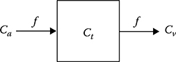
FIGURE 17.1
Single-tissue compartment model for H₂¹⁵O. C_t is the tissue concentration of H₂¹⁵O (μCi/g), C_a the arterial concentration of H₂¹⁵O (μCi/mL), C_v the venous concentration of H₂¹⁵O (μCi/mL), and f the blood flow per unit weight of tissue (mL/min/g).

Assuming that water is freely diffusible in the tissue space, and that the ¹⁵O distribution reaches equilibrium instantaneously, venous concentration is related to the tissue concentration by

C_{v} (t) = \frac{1}{p} C_{t} (t) (17.2)

$C_{v} (t) = \frac{1}{p} C_{t} (t) (17.2)$

where p is tissue/blood partition coefficient (mL/g), which is a measurement of the ratio of the water content in the tissue to that in the blood at equilibrium. Inserting Equation 17.2 into Equation 17.1 gives

\frac{d C_{t} (t)}{d t} = f \cdot C_{a} (t) - \frac{f}{p} C_{t} (t) (17.3)

$\frac{d C_{t} (t)}{d t} = f \cdot C_{a} (t) - \frac{f}{p} C_{t} (t) (17.3)$

Solving differential Equation 17.3 for C_t(t) gives

C_{t} (t) = f \int_{0}^{t} C_{a} (τ) \cdot e^{- \frac{f}{p} (t - τ)} d τ = f \cdot C_{a} (t) \otimes e^{- \frac{f}{p} \times t} (17.4)

$C_{t} (t) = f \int_{0}^{t} C_{a} (τ) \cdot e^{- \frac{f}{p} (t - τ)} d τ = f \cdot C_{a} (t) \otimes e^{- \frac{f}{p} \times t} (17.4)$

where C_t(t = 0) = 0 is assumed, and ⊗ denotes the convolution integral. Figure 17.2 illustrates tissue time-activity curves of various blood flow values, being generated using Equation 17.4.

Images

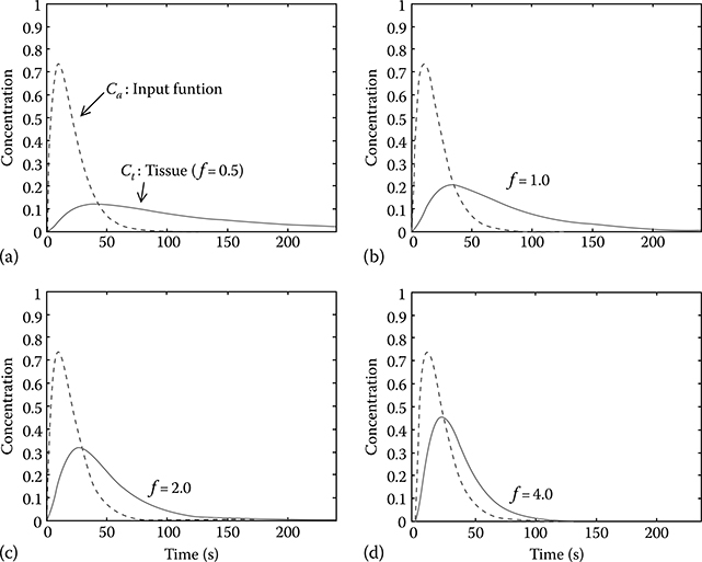
FIGURE 17.2
Tissue time–activity curves with different values of blood flow (f) as described by Equation 17.4 (partition coefficient p is fixed at 0.9). (a) f = 0.5, (b) f = 1.0, (c) f = 2.0, and (d) f = 4.0.

In terms of the measurement of cerebral blood flow, two unknown parameters, blood flow (f) and partition coefficient (p), are commonly estimated.

In the measurement of myocardial blood flow, the measured tissue time–activity curves by PET can be related to the ideal one by incorporating the partial volume and spillover effects^7,8:

{\tilde{C}}_{t} (t) = α \cdot C_{t} (t) + V_{a} \cdot C_{a} (t) = α \cdot f \cdot C_{a} (t) \otimes e^{- \frac{f}{p} \times t} + V_{a} \times C_{a} (t) (17.5)

${\tilde{C}}_{t} (t) = α \cdot C_{t} (t) + V_{a} \cdot C_{a} (t) = α \cdot f \cdot C_{a} (t) \otimes e^{- \frac{f}{p} \times t} + V_{a} \times C_{a} (t) (17.5)$

where

α is the perfusible tissue fraction (PTF, g/mL) or recovery coefficient for the partial volume correction of the tissue time–activity curve

V_a is the arterial blood volume fraction (mL/mL) of the ROI. By fixing p (= 0.91 mL/g), three unknown parameters (α, f, V_a) can be estimated

17.2.2.1.2 Glucose Metabolism

¹⁸F-FDG, an ¹⁸F-labeled analogue of glucose, is a tracer used to study glucose metabolism by PET. FDG enters the tissue and is phosphorylated into FDG-6-phosphate (FDG-6-PO₄), which cannot be further metabolized by the glycolytic pathway. Therefore, a three-compartment model (a two-tissue compartment model) is commonly used for ¹⁸F-FDG (Figure 17.3).⁹

This system can be described by the following set of differential equations:

\frac{d C_{e} (t)}{d t} = K_{1} C_{p} (t) - k_{2} C_{e} (t) - k_{3} C_{e} (t) + k_{4} C_{m} (t) (17.6)

$\frac{d C_{e} (t)}{d t} = K_{1} C_{p} (t) - k_{2} C_{e} (t) - k_{3} C_{e} (t) + k_{4} C_{m} (t) (17.6)$

\frac{d C_{m} (t)}{d t} = k_{3} C_{e} (t) - k_{4} C_{m} (t) (17.7)

$\frac{d C_{m} (t)}{d t} = k_{3} C_{e} (t) - k_{4} C_{m} (t) (17.7)$

where

C_p(t) is the plasma concentration of FDG (μCi/mL)

C_e(t) is the concentration of exchangeable FDG (μCi/g)

C_m(t) is the concentration of FDG-6-PO₄ (μCi/g)

Images

FIGURE 17.3
Three-compartment (two-tissue compartment) model for ¹⁸F-FDG. C_p is the plasma concentration of FDG (μCi/mL), C_e the concentration of exchangeable FDG (μCi/g), and C_m the concentration of FDG-6-PO₄ (μCi/g). The rate constants K₁, k₂, k₃, and k₄ are defined as delivery (mL/min/g), washout (min⁻¹), phosphorylation of FDG (min⁻¹), and dephosphorylation of FDG-6-P (min⁻¹), respectively.

The rate constants K₁, k₂, k₃, and k₄ are defined as delivery (mL/min/g), washout (min⁻¹), phosphorylation of FDG (min⁻¹), and dephosphorylation of FDG-6-P (min⁻¹), respectively.

The measured tissue time–activity curve by PET is the sum of the solution of the aforementioned two equations¹⁰:

\begin{matrix} C_{t} (t) = C_{e} (t) + C_{m} (t) = K_{1} C_{p} (t) \otimes [(\frac{k_{3} + k_{4} - q_{1}}{q_{2} - q_{1}}) e^{- q_{1} t} - (\frac{k_{3} + k_{4} - q_{2}}{q_{2} - q_{1}}) e^{- q_{2} t}] \\ q_{1}, q_{2} = \frac{(k_{2} + k_{3} + k_{4}) \mp \sqrt{{(k_{2} + k_{3} + k_{4})}^{2} - 4 k_{2} k_{4}}}{2} \end{matrix} (17.8)

$\begin{matrix} C_{t} (t) = C_{e} (t) + C_{m} (t) = K_{1} C_{p} (t) \otimes [(\frac{k_{3} + k_{4} - q_{1}}{q_{2} - q_{1}}) e^{- q_{1} t} - (\frac{k_{3} + k_{4} - q_{2}}{q_{2} - q_{1}}) e^{- q_{2} t}] \\ q_{1}, q_{2} = \frac{(k_{2} + k_{3} + k_{4}) \mp \sqrt{{(k_{2} + k_{3} + k_{4})}^{2} - 4 k_{2} k_{4}}}{2} \end{matrix} (17.8)$

Making the assumption that k₄ is zero (the dephosphorylation of FDG-6-PO₄ is relatively slow), the analytic solution of the tissue time–activity curve is described by

C_{t} (t) = \frac{K_{1}}{k_{2} + k_{3}} C_{p} (t) \otimes [k_{3} + k_{2} e^{- (k_{2} + k_{3}) t}] (17.9)

$C_{t} (t) = \frac{K_{1}}{k_{2} + k_{3}} C_{p} (t) \otimes [k_{3} + k_{2} e^{- (k_{2} + k_{3}) t}] (17.9)$

Individual rate constants can be estimated using linear or nonlinear regression analysis to fit the aforementioned equation to the measured tissue time–activity curve. The net transport rate (K_in) of FDG, K₁k₃/(k₂+k₃), can be calculated using individual rate constants determined by the regression analysis of Equation 17.8 or 17.9, or by Gjedde-Patlak graphical analysis.^11–13

Finally, the glucose utilization rate is obtained using the following equation:

\frac{1}{L C} \frac{K_{1} k_{3}}{k_{2} + k_{3}} C_{p} (17.10)

$\frac{1}{L C} \frac{K_{1} k_{3}}{k_{2} + k_{3}} C_{p} (17.10)$

where

LC is a lumped constant, which is used to calibrate the differences in transport and phosphorylation between FDG and glucose

C_p represents the glucose concentration in blood^9,14

17.2.2.1.3 Receptor-Ligand Binding

The concentration of receptors (B_max) and the equilibrium dissociation constant (K_d) for the specific binding of ligands to receptors, or their ratios (binding potentials) can be estimated using the compartment modeling method with a plasma compartment and three tissue compartments (free, nonspecific binding, and specific binding, respectively).^14,15 If the exchange between the free and nonspecific compartments is rapid enough and/or the nonspecific binding is small relative to the free compartment, the model can be reduced to a two-tissue compartment model.¹⁶ Each compartment in this model represents the concentration of radioligand in plasma (C_p_, μCi/mL), free or nonspecifically bound radioligand (C_f_, μCi/g), and radioligand specifi-cally bound by receptors (C_b_, μCi/g) (Figure 17.4).

Images

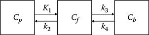
FIGURE 17.4
Three-compartment (two-tissue compartment) model for a receptor-rich region. C_p is the concentration of radioligand in plasma (μCi/mL), C_f the free or nonspecifically bound radioli-gand (μCi/g), and C_b the radioligand specifically bound by receptors (μCi/g). The rate constants K₁, k₂, k₃, and k₄ are defined as the delivery (mL/min/g), washout (min⁻¹), forward receptor–ligand reaction (min⁻¹), and reverse receptor–ligand reaction (min⁻¹), respectively.

Changes in C_f and C_b are described by

\frac{d C_{f} (t)}{d t} = K_{1} C_{p} (t) - k_{2} C_{f} (t) - k_{3} (t) C_{f} (t) + k_{4} C_{b} (t) (17.11)

$\frac{d C_{f} (t)}{d t} = K_{1} C_{p} (t) - k_{2} C_{f} (t) - k_{3} (t) C_{f} (t) + k_{4} C_{b} (t) (17.11)$

\begin{matrix} \frac{d C_{b} (t)}{d t} = k_{3} (t) C_{f} (t) - k_{4} C_{b} (t) \\ k_{3} (t) = k_{o n} (B_{\max} - \frac{C_{b} (t)}{S A}), k_{4} = k_{o f f} \end{matrix} (17.12)

$\begin{matrix} \frac{d C_{b} (t)}{d t} = k_{3} (t) C_{f} (t) - k_{4} C_{b} (t) \\ k_{3} (t) = k_{o n} (B_{\max} - \frac{C_{b} (t)}{S A}), k_{4} = k_{o f f} \end{matrix} (17.12)$

where the rate constants K₁, k₂, k₃, and k₄ are defined as the delivery (mL/min/g), washout (min⁻¹), forward receptor-ligand reaction (min⁻¹), and reverse receptor-ligand reaction (min⁻¹), respectively. k_on is the bimolecular association rate constant (g/pmol/min), k_off the unimolecular dissociation rate constant (min⁻¹), B_max the density of receptor sites available for radio-ligand binding (apparent B_max, pmol/g), and SA the specific activity (radio activity per mole of a labeled compound, μCi/pmol).^17,18

If the SA is high, then C_b(t)/SA (occupancy of receptors by the labeled compound) is negligibly small, k₃(t) (= k_on(B_max – C_b(t)/SA)) can then be approximated by k_onB_max, and the above Equations 17.11 and 17.12 can be written as a first-order equation without the (C_b(t)C_f(t)) multiplication term and an analytical solution can be derived (the same form as Equation 17.8). Otherwise, the analytic solution of this equation cannot be simply obtained. Numerical solutions for C_f and C_b are, therefore, required for time–activity curves with low SA. Binding potential (BP) is obtained from B_max/K_d = k_onB_max/k_off, and is equal to k₃/k₄ for high SA data.

In imaging studies, volume of distribution is the ratio of the concentration of radiotracer in a region of tissue to that in plasma at equilibrium. At equilibrium, also the Equations 17.11 and 17.12 will be zero. Thus, the volume of distribution of each compartment in Figure 17.4 and their sum can be related with the rate constants as follows:

V_{f} = \frac{C_{f}}{C_{p}} = \frac{K_{1}}{k_{2}} (17.13)

$V_{f} = \frac{C_{f}}{C_{p}} = \frac{K_{1}}{k_{2}} (17.13)$

V_{b} = \frac{C_{b}}{C_{p}} = \frac{K_{1} k_{3}}{k_{2} k_{4}} (17.14)

$V_{b} = \frac{C_{b}}{C_{p}} = \frac{K_{1} k_{3}}{k_{2} k_{4}} (17.14)$

V_{t} = V_{f} + V_{b} = \frac{K_{1}}{k_{2}} (1 + \frac{k_{3}}{k_{4}}) (17.15)

$V_{t} = V_{f} + V_{b} = \frac{K_{1}}{k_{2}} (1 + \frac{k_{3}}{k_{4}}) (17.15)$

Consequently, the BP can be related with the volume of distribution or their ratio (distribution volume ratio: DVR) as follows:

B P = \frac{V_{b}}{V_{f}} = \frac{V_{t} - V_{f}}{V_{f}} = \frac{V_{t}}{V_{f}} - 1 = D V R - 1 (17.16)

$B P = \frac{V_{b}}{V_{f}} = \frac{V_{t} - V_{f}}{V_{f}} = \frac{V_{t}}{V_{f}} - 1 = D V R - 1 (17.16)$

For some radioligands, reference regions that do not have high-affinity receptors are available. The single-tissue compartment model is used for such reference regions (Figure 17.5). If we assume that the distribution volumes of free and nonspecifically bound radioligand in an ROI and in a reference region are the same (K₁/k₂ = K′₁/k′₂) for some radioligands, biological constraint can be applied to improve the stability of rate constant estimates or to replace the arterial input function by the time–activity curve for a reference region. The ratio of K′₁ and k′₂ which are obtained by fitting the time–activity curve from the reference region, can be fixed during rate constant estimation for ROIs.^19,20

The reference tissue model is a method in which this constraint is used to derive the relationship between the time–activity curves of an ROI and of reference tissue; moreover, the analytical solution of the time–activity curves for an ROI can be fitted without an arterial input function.²¹ Lammertsma and Hume derived the following equation for the tracer (i.e., [¹¹C]raclopride), the kinetics of which cannot be distinguished in free (+ nonspecific) and specific compartments, since the exchange of tracer between those two compartments is rapid compared to that between plasma and free compartments (simplified reference tissue model).²²

Images

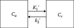
FIGURE 17.5
Two-compartment (single-tissue compartment) for a reference region: C_r is the concentration of the free or nonspecifically bound radioligand in the reference region (μCi/g).

C_{t} (t) = R_{1} C_{r} (t) + {k_{2} - \frac{R_{1} k_{2}}{(1 + B P)}} C_{r} (t) \otimes e^{\frac{- k_{2} t}{(1 + B P)}} (17.17)

$C_{t} (t) = R_{1} C_{r} (t) + {k_{2} - \frac{R_{1} k_{2}}{(1 + B P)}} C_{r} (t) \otimes e^{\frac{- k_{2} t}{(1 + B P)}} (17.17)$

where R₁ = k₁/k₂ and BP is k₃/k₄.

17.2.2.2 Noncompartmental Modeling

In the noncompartmental approach, specific kinetic parameters are estimated without the detailed compartmentalization of the system.⁴ The complexity of the systems is usually lumped into some macro parameters. Graphical analysis is an example of this approach, in which the differential equations of compartmental analysis are converted into linear plots.^{11–13,23–25} The slope and intercept of these plots are then used to determine the kinetic parameters. Spectral analysis is another method used for PET/SPECT data, in which the model is not strictly constrained by the number of compartments and the relationship between compartments.^26,27

17.2.2.2.1 Graphical Analysis

Although the graphical methods are independent of particular model structures, if a model structure describes the transfer of tracer, the slope of the linear equation can be related to combinations of the model parameters.²³ Since linear regression is employed in graphical analysis, it requires only the computation of the analytic solution of the slopes. The Gjedde-Patlak plot is the most widely used method for irreversibly binding tracers (Figure 17.6a).^11–13 If the transport of a tracer to the third compartment is irreversible (k₄ = 0), differential equations (i.e., Equations 17.6 and 17.7) for the three-compartment model can be rearranged into the following equation:

\frac{C_{t} (t)}{C_{p} (t)} = \frac{K_{1} k_{3}}{k_{2} + k_{3}} \frac{\int_{0}^{t} C_{p} (τ) d τ}{C_{p} (t)} + V_{e}, (17.18)

$\frac{C_{t} (t)}{C_{p} (t)} = \frac{K_{1} k_{3}}{k_{2} + k_{3}} \frac{\int_{0}^{t} C_{p} (τ) d τ}{C_{p} (t)} + V_{e}, (17.18)$

for t > t′ when the distribution volume of the reversible part (V_e) is constant.

The slope of the aforementioned equation equals to the net transfer rate of tracer from plasma to the irreversible compartment.

For the quantification of reversible tracers (k₄ ≠ 0), Logan graphical methods are used to determine the distribution volumes of reference region and region with specific binding and/or their ratio with or without the arterial input function (Figure 17.6b).^24,25 The Logan equation for specific binding region shown in Figure 17.4 is

Images

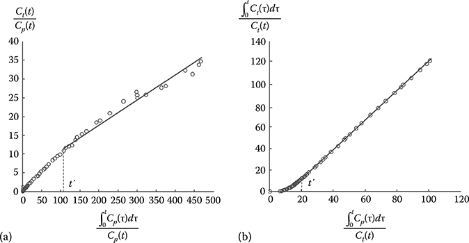
FIGURE 17.6
Graphical analysis. (a) Gjedde-Patlak plot. (b) Logan plot.

\frac{\int_{0}^{t} C_{t} (τ) d τ}{C_{t} (t)} = \frac{K_{1}}{k_{2}} (1 + \frac{k_{3}}{k_{4}}) \frac{\int_{0}^{t} C_{p} (τ) d τ}{C_{t} (t)} + b = V_{t} \frac{\int_{0}^{t} C_{p} (τ) d τ}{C_{t} (t)} + b, (17.19)

$\frac{\int_{0}^{t} C_{t} (τ) d τ}{C_{t} (t)} = \frac{K_{1}}{k_{2}} (1 + \frac{k_{3}}{k_{4}}) \frac{\int_{0}^{t} C_{p} (τ) d τ}{C_{t} (t)} + b = V_{t} \frac{\int_{0}^{t} C_{p} (τ) d τ}{C_{t} (t)} + b, (17.19)$

for t > t′ when the intercept b becomes constant.

For reference region with no specific binding (Figure 17.5), the Logan plot can be represented as follows:

\frac{\int_{0}^{t} C_{r} (τ) d τ}{C_{r} (t)} = \frac{{K^{'}}_{1}}{{k^{'}}_{2}} \frac{\int_{0}^{t} C_{p} (τ) d τ}{C_{r} (t)} + b (17.20)

$\frac{\int_{0}^{t} C_{r} (τ) d τ}{C_{r} (t)} = \frac{{K^{'}}_{1}}{{k^{'}}_{2}} \frac{\int_{0}^{t} C_{p} (τ) d τ}{C_{r} (t)} + b (17.20)$

By substituting the integral term of input function that can be obtained from Equation 17.19 into Equation 17.20 with the assumption of K₁/k₂ = K′₁/k′₂, we can also derive the following equation in which the reference tissue time–activity curve is regarded as input function:

\frac{\int_{0}^{t} C_{t} (t) d t}{C_{t} (t)} = D V R \frac{\int_{0}^{t} C_{r} (t) d t}{C_{t} (t)} + b (17.21)

$\frac{\int_{0}^{t} C_{t} (t) d t}{C_{t} (t)} = D V R \frac{\int_{0}^{t} C_{r} (t) d t}{C_{t} (t)} + b (17.21)$

where the slope, DVR, is the distribution volume ratio.

17.2.2.2.2 Spectral Analysis

In the case of a new tracer of unknown kinetics, noncompartmental tracer kinetic modeling techniques are necessary initially to identify the kinetic components present in the measured data and to determine the pharma-cokinetic variables with relatively few model assumptions. Data-driven approaches like spectral analysis can be used for this purpose.^26,27

In spectral analysis, the observed time course of a labeled drug is fitted using a linear combination of possible tissue response curves, each of which is a single exponential in time convolved with the input function C_p:

C_{t} (t) = \frac{1}{t_{i + 1} - t_{i}} \int_{t_{i}}^{t_{i + 1}} (\sum_{j = 1}^{N} C_{p} (τ) \otimes α_{j} e^{- β_{t} t}) d t (α_{j} \geq 0, λ \leq β_{j} \leq 1) (17.22)

$C_{t} (t) = \frac{1}{t_{i + 1} - t_{i}} \int_{t_{i}}^{t_{i + 1}} (\sum_{j = 1}^{N} C_{p} (τ) \otimes α_{j} e^{- β_{t} t}) d t (α_{j} \geq 0, λ \leq β_{j} \leq 1) (17.22)$

where

N is the maximal number of basis functions allowed in the model

λ is the decay constant of the radioisotope

the t_i (i = 1, …, n) values are the frame times

Values of α are determined, which best fit the measured data at predefined β values on the interval [λ, 1(fastest measurable dynamic)]. The fitted values of α, together with the corresponding chosen values of β, define the tissue unit impulse-response function:

h (t) = \sum_{j = 1}^{N} α_{j} e^{- (β_{j} - λ) t} (17.23)

$h (t) = \sum_{j = 1}^{N} α_{j} e^{- (β_{j} - λ) t} (17.23)$

from which the pharmacokinetic parameters can be calculated as follows:

K_{1} = h (0) = \sum_{j = 1}^{N} α_{j}, V D = \int_{0}^{\infty} h (τ) d τ = \sum_{j = 1}^{N} \frac{α_{j}}{β_{j} - λ}, M R T = \frac{V D}{K_{1}} (17.24)

$K_{1} = h (0) = \sum_{j = 1}^{N} α_{j}, V D = \int_{0}^{\infty} h (τ) d τ = \sum_{j = 1}^{N} \frac{α_{j}}{β_{j} - λ}, M R T = \frac{V D}{K_{1}} (17.24)$

where

K₁ is the rate constant for the delivery of tracer from the plasma to tissue

VD is the fractional volume of the distribution

MRT is the mean residence time of the tracer in the sampled tissue²⁷

17.3 Parameter Estimation and Parametric Images

To estimate unknown parameters (i.e., rate constants) from the tissue time–activity curves and input function, these parameters are conventionally fitted by nonlinear least squares (NLS) analysis. However, the result of the parameter estimation using NLS is dependent on the initial guessing of parameters. Thus, a poor initial guess results in an incorrect result at local minima of the cost function and slow convergence. In addition, an appropriate convergence threshold and constraints on the parameters should be determined by experience. The NLS method also requires considerable computation time to estimate parameters.²⁸ This method is, therefore, impractical for a pixel-by-pixel analysis designed to generate parametric images of these parameters, which is important for clinical and research purposes, since parametric images provide us with anatomically oriented information about the kinetic parameters, without the spatial resolution loss associated with the ROI method. Thus, the linear analysis methods, such as graphical analysis, linear least squares (LLS), and linear weighted least squares (LWLS) are commonly used for generating parametric images.

In weighted least squares methods, the structure of the error variance can be concerned by weighting the measurement error with the relative accuracy of the measurement.²⁸ However, direct estimation of the error variance of every pixel is hard to achieve practically. An approximate weighting formula is, therefore, commonly used.^29,30 Generalized least squares (GLS) and gen-eralized weighted least squares (GWLS) are the generalized formula of LLS and LWLS, respectively. Since the dependency between the measurement error at each sampling point in the LLS and LWLS methods leads to bias in the estimated parameters, GLS and GWLS were suggested as alternatives to eliminate this bias.^29,30

17.3.1 Nonlinear least Squares (NlS)

Let us begin explain these methods using an example of the single-tissue compartment model with two unknown parameters (K₁ and k₂). Recall that the model equation for the single-tissue compartment model with two parameters is described by Equation 17.3. Replacing f and f/p with K₁ and k₂, respectively,

\frac{d C_{t} (t)}{d t} = K_{1} C_{a} (t) - k_{2} C_{t} (t) (17.25)

$\frac{d C_{t} (t)}{d t} = K_{1} C_{a} (t) - k_{2} C_{t} (t) (17.25)$

The solution of Equation 17.25 is

C_{t} (t) = K_{1} C_{a} (t) \otimes e^{- k_{2} t} (17.26)

$C_{t} (t) = K_{1} C_{a} (t) \otimes e^{- k_{2} t} (17.26)$

Parameter estimation is performed by defining an optimization cost function and then by choosing those parameter values that minimize the function. The most common cost function is the residual sum of squares, which is the sum of the squared deviations between the measured tissue time–activity curve and predicted tissue time–activity curve obtained using estimated parameters (Figure 17.7). When the NLS method is used, the parameters are varied iteratively using a Gaussian–Newton or a Levenberg–Marquardt algorithm until the following residual sum of squares reaches a minimum.^31,32

Images

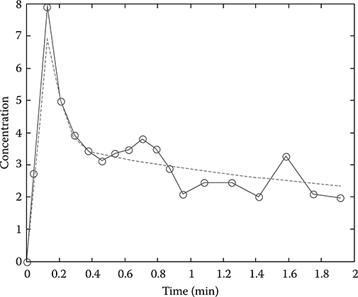
FIGURE 17.7
Parameter estimation by curve fitting. Circles on solid line represent the measured data and dashed line is the fitted (or predicted) tissue time–activity curve.

\sum_{i = 1}^{n} w_{i} {[C_{t} (t_{i}) - K_{1} C_{a} (t) \otimes e^{- k_{2} t}]}^{2} (17.27)

$\sum_{i = 1}^{n} w_{i} {[C_{t} (t_{i}) - K_{1} C_{a} (t) \otimes e^{- k_{2} t}]}^{2} (17.27)$

where w_i is the weight associated with the ith measurement, and reflects the relative accuracy of the measurement. The aforementioned equation is general formulation, which describes the structure of the error variance, and the technique is called nonlinear weighted least squares. If we set all w_i values to be equal, the method is simply called nonlinear least squares.

Under the assumptions of a zero mean, an uncorrelated measurement error, and errorless independent variables, the optimal choice of weights is²⁸

w_{i} = V a r {(e_{i})}^{- 1} (17.28)

$w_{i} = V a r {(e_{i})}^{- 1} (17.28)$

where e_i is the error in ith measurement.

17.3.2 linear least Squares (llS)

17.3.2.1 Single-Tissue Compartment Models

Integrating Equation 17.25 from time 0 to t_i, where t_i = t₁, t₂, …, t_n are the sampling times of the tissue measurements, gives

\begin{matrix} C_{t} (t_{1}) = K_{1} \int_{0}^{t_{1}} C_{a} (τ) d τ - k_{2} \int_{\overset{\leftarrow}{0}}^{t_{1}} C_{t} (τ) d τ + ε_{1} \\ C_{t} (t_{2}) = K_{1} \int_{0}^{t_{2}} C_{a} (τ) d τ - k_{2} \int_{0}^{t_{2}} C_{t} (τ) d τ + ε_{2} \\ ⋮ \\ C_{t} (t_{n}) = K_{1} \int_{0}^{t_{n}} C_{a} (τ) d τ - k_{2} \int_{0}^{t_{n}} C_{t} (τ) d τ + ε_{n} \end{matrix} (17.29)

$\begin{matrix} C_{t} (t_{1}) = K_{1} \int_{0}^{t_{1}} C_{a} (τ) d τ - k_{2} \int_{\overset{\leftarrow}{0}}^{t_{1}} C_{t} (τ) d τ + ε_{1} \\ C_{t} (t_{2}) = K_{1} \int_{0}^{t_{2}} C_{a} (τ) d τ - k_{2} \int_{0}^{t_{2}} C_{t} (τ) d τ + ε_{2} \\ ⋮ \\ C_{t} (t_{n}) = K_{1} \int_{0}^{t_{n}} C_{a} (τ) d τ - k_{2} \int_{0}^{t_{n}} C_{t} (τ) d τ + ε_{n} \end{matrix} (17.29)$

where ∊₁, ∊₂, …, ∊_n are error terms.

These equations can be considered a set of linear equations in which the time integration of the input function and of the tissue time–activity curve are independent variables, the instantaneous tissue time–activity curve value is a dependent variable, and K₁ and k₂ are its coefficients.

Rearranging these equations into a matrix form gives

y = X θ + ε (17.30)

$y = X θ + ε (17.30)$

where

y \equiv {[C_{t} (t_{1}) C_{t} (t_{2}) \dots C_{t} (t_{n})]}^{T} (17.31)

$y \equiv {[C_{t} (t_{1}) C_{t} (t_{2}) \dots C_{t} (t_{n})]}^{T} (17.31)$

X \equiv [\begin{matrix} \int_{0}^{t_{1}} C_{a} (τ) d τ & \int_{0}^{t_{1}} C_{t} (τ) d τ \\ \int_{0}^{t_{2}} C_{a} (τ) d τ & \int_{0}^{t_{2}} C_{t} (τ) d τ \\ ⋮ & ⋮ \\ \int_{0}^{t_{n}} C_{a} (τ) d τ & \int_{0}^{t_{n}} C_{t} (τ) d τ \end{matrix}] (17.32)

$X \equiv [\begin{matrix} \int_{0}^{t_{1}} C_{a} (τ) d τ & \int_{0}^{t_{1}} C_{t} (τ) d τ \\ \int_{0}^{t_{2}} C_{a} (τ) d τ & \int_{0}^{t_{2}} C_{t} (τ) d τ \\ ⋮ & ⋮ \\ \int_{0}^{t_{n}} C_{a} (τ) d τ & \int_{0}^{t_{n}} C_{t} (τ) d τ \end{matrix}] (17.32)$

ε \equiv {[ε_{1} ε_{2} \dots ε_{n}]}^{T} (17.33)

$ε \equiv {[ε_{1} ε_{2} \dots ε_{n}]}^{T} (17.33)$

θ \equiv {[K_{1} - k_{2}]}^{T} (17.34)

$θ \equiv {[K_{1} - k_{2}]}^{T} (17.34)$

If we assume that the error terms are independent of each other, an estimate of θ can be obtained by using the following equation:

{\overset{⌢}{θ}}_{LLS} = {(X^{T} X)}^{- 1} X^{T} y (17.35)

${\overset{⌢}{θ}}_{LLS} = {(X^{T} X)}^{- 1} X^{T} y (17.35)$

Suppose that the variance is not constant, the estimate θ then is

{\overset{⌢}{θ}}_{LWLS} = {(X^{T} W X)}^{- 1} X^{T} W y (17.36)

${\overset{⌢}{θ}}_{LWLS} = {(X^{T} W X)}^{- 1} X^{T} W y (17.36)$

where W is an n by n diagonal matrix consisting of the weights w_i. This later method is called the linear weighted least squares (LWLS) method.

Although error terms in Equation 17.29 are assumed to be mutually independent, the assumption is incorrect since the integration periods overlap so that the later error terms contain previous errors. This dependency between error terms leads to a bias in the estimated parameters when the LLS method is used. The GLS method was suggested to overcome this bias problem.^29,30 GLS iteratively upgrades the estimates, which are initially obtained from the LLS, and the final estimates are unbiased. The GLS estimate is given as

{\hat{θ}}_{GLS} = {(Z^{T} Z)}^{- 1} Z^{T} r (17.37)

${\hat{θ}}_{GLS} = {(Z^{T} Z)}^{- 1} Z^{T} r (17.37)$

where

r \equiv [\begin{matrix} C_{t} (t_{1}) - {\hat{k}}_{2} C_{t} (t_{1}) \otimes e^{- {\hat{k}}_{2} t_{1}} \\ C_{t} (t_{2}) - {\hat{k}}_{2} C_{t} (t_{2}) \otimes e^{- {\hat{k}}_{2} t_{2}} \\ ⋮ \\ C_{t} (t_{n}) - {\hat{k}}_{2} C_{t} (t_{n}) \otimes e^{- {\hat{k}}_{2} t_{n}} \end{matrix}] (17.38)

$r \equiv [\begin{matrix} C_{t} (t_{1}) - {\hat{k}}_{2} C_{t} (t_{1}) \otimes e^{- {\hat{k}}_{2} t_{1}} \\ C_{t} (t_{2}) - {\hat{k}}_{2} C_{t} (t_{2}) \otimes e^{- {\hat{k}}_{2} t_{2}} \\ ⋮ \\ C_{t} (t_{n}) - {\hat{k}}_{2} C_{t} (t_{n}) \otimes e^{- {\hat{k}}_{2} t_{n}} \end{matrix}] (17.38)$

Z \equiv [\begin{matrix} C_{a} (t_{1}) \otimes e^{- {\hat{k}}_{2} t_{1}} & C_{t} (t_{1}) \otimes e^{- {\hat{k}}_{2} t_{1}} \\ C_{a} (t_{2}) \otimes e^{- {\hat{k}}_{2} t_{2}} & C_{t} (t_{2}) \otimes e^{- {\hat{k}}_{2} t_{2}} \\ ⋮ & ⋮ \\ C_{a} (t_{n}) \otimes e^{- {\hat{k}}_{2} t_{n}} & C_{t} (t_{n}) \otimes e^{- {\hat{k}}_{2} t_{n}} \end{matrix}] (17.39)

$Z \equiv [\begin{matrix} C_{a} (t_{1}) \otimes e^{- {\hat{k}}_{2} t_{1}} & C_{t} (t_{1}) \otimes e^{- {\hat{k}}_{2} t_{1}} \\ C_{a} (t_{2}) \otimes e^{- {\hat{k}}_{2} t_{2}} & C_{t} (t_{2}) \otimes e^{- {\hat{k}}_{2} t_{2}} \\ ⋮ & ⋮ \\ C_{a} (t_{n}) \otimes e^{- {\hat{k}}_{2} t_{n}} & C_{t} (t_{n}) \otimes e^{- {\hat{k}}_{2} t_{n}} \end{matrix}] (17.39)$

Equation 17.37 is used repeatedly with ${\hat{k}}_{2}$ ${\hat{k}}_{2}$ updated for each iteration.

As for the LWLS method, the GWLS estimate is

{\overset{⌢}{θ}}_{GWLS} = {(Z^{T} W Z)}^{- 1} Z^{T} W r (17.40)

${\overset{⌢}{θ}}_{GWLS} = {(Z^{T} W Z)}^{- 1} Z^{T} W r (17.40)$

where r and Z have the forms shown in Equations 17.38 and 17.39.

This LLS and related estimation methods can be also applied to the extended model for incorporating the partial volume and spillover effects.³³ From Equation 17.5, the ideal time–activity curves can be expressed with the measured time–activity curves according to the following equations:

C_{a} (t) = {\tilde{C}}_{a} (t) (17.41)

$C_{a} (t) = {\tilde{C}}_{a} (t) (17.41)$

C_{t} (t) = \frac{{\tilde{C}}_{t} (t) - V_{a} \cdot {\tilde{C}}_{a} (t)}{α} (17.42)

$C_{t} (t) = \frac{{\tilde{C}}_{t} (t) - V_{a} \cdot {\tilde{C}}_{a} (t)}{α} (17.42)$

Substituting the aforementioned two equations into Equation 17.25, and multiplying both sides by α,

\frac{d}{d t} {{\tilde{C}}_{t} (t) - V_{a} \cdot {\tilde{C}}_{a} t} = K_{1} \cdot {\tilde{C}}_{a} (t) - k_{2} {{\tilde{C}}_{t} (t) - V_{a} \cdot {\tilde{C}}_{a} (t)} (17.43)

$\frac{d}{d t} {{\tilde{C}}_{t} (t) - V_{a} \cdot {\tilde{C}}_{a} t} = K_{1} \cdot {\tilde{C}}_{a} (t) - k_{2} {{\tilde{C}}_{t} (t) - V_{a} \cdot {\tilde{C}}_{a} (t)} (17.43)$

where K₁ is the product of α and f.

Rearranging this equation and integrating both sides from time 0 to each PET sampling point yields the following linear equation:

{\tilde{C}}_{t} (t) = P_{1} \cdot {\tilde{C}}_{a} (t) + P_{2} \int_{0}^{t} {\tilde{C}}_{a} (τ) d τ + P_{3} \int_{0}^{t} {\tilde{C}}_{t} (τ) d τ (17.44)

${\tilde{C}}_{t} (t) = P_{1} \cdot {\tilde{C}}_{a} (t) + P_{2} \int_{0}^{t} {\tilde{C}}_{a} (τ) d τ + P_{3} \int_{0}^{t} {\tilde{C}}_{t} (τ) d τ (17.44)$

\begin{matrix} P_{1} \equiv V_{a} \\ P_{2} \equiv K_{1} + k_{2} \cdot V_{a} \\ P_{3} \equiv - k_{2} \end{matrix} (17.45)

$\begin{matrix} P_{1} \equiv V_{a} \\ P_{2} \equiv K_{1} + k_{2} \cdot V_{a} \\ P_{3} \equiv - k_{2} \end{matrix} (17.45)$

Figure 17.8 shows the parametric image of K₁ generated from the dynamic myocardial H₂¹⁵O PET image using the method described earlier.³³

Images

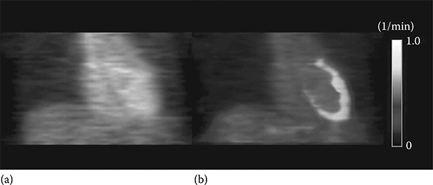
FIGURE 17.8
(See color insert.) Parametric image of K₁ generated from dynamic H₂¹⁵O PET using linear least squares method. (a) Static PET image. (b) K₁ parametric image superimposed on static image. (Modified from Figure 17.5 in Lee JS, et al., J Nucl Med. 2005, 46(10), 1687–1695 ^© by the Society of Nuclear Medicine, Inc.)

17.3.2.2 Two-Tissue Compartment Models

17.3.2.2.1 Irreversible Binding

From differential equations of the two-tissue compartment model with irreversible binding, two multiple linear regression model equations can be derived.³⁴ The functional equation of the first formula (multiple linear analysis for irreversible radiotracer 1: MLAIR1) takes the form:

C_{t} (t) = P_{1} C_{p} (t) + P_{2} \int_{0}^{t} C_{p} (τ) d τ + P_{3} \int_{0}^{t} C_{t} (τ) d τ + P_{4} \int_{0}^{t} \int_{0}^{τ} C_{p} (s) d s d τ (17.46)

$C_{t} (t) = P_{1} C_{p} (t) + P_{2} \int_{0}^{t} C_{p} (τ) d τ + P_{3} \int_{0}^{t} C_{t} (τ) d τ + P_{4} \int_{0}^{t} \int_{0}^{τ} C_{p} (s) d s d τ (17.46)$

where the macro parameters P₁ ∼ P₄ are given by

\begin{matrix} P_{1} = V_{a} \\ P_{2} = K_{1} + k_{2} V_{a} + k_{3} V_{a} \\ P_{3} = - (k_{2} + k_{3}) \\ P_{4} = K_{1} k_{3} \end{matrix} (17.47)

$\begin{matrix} P_{1} = V_{a} \\ P_{2} = K_{1} + k_{2} V_{a} + k_{3} V_{a} \\ P_{3} = - (k_{2} + k_{3}) \\ P_{4} = K_{1} k_{3} \end{matrix} (17.47)$

The net accumulation rate K_in can then be acquired using the following equation:

K_{i n} = \frac{K_{1} k_{3}}{k_{2} + k_{3}} = - \frac{P_{4}}{P_{3}} (17.48)

$K_{i n} = \frac{K_{1} k_{3}}{k_{2} + k_{3}} = - \frac{P_{4}}{P_{3}} (17.48)$

The MLAIR1 is a useful alternative to the Gjedde-Patlak plot because the determination of a linear interval is not necessary. However, the error propagation associated with the division calculation on the macro parameters (Equation 17.48), to obtain K_in, is a possible limitation of MLAIR1 for the voxel-wise estimations of K_in for the generation of parametric images because of the high noise level in the individual time–activity curves of each voxel. On the contrary, MLAIR2 is a formula in which K_in could be directly estimated from the coefficient of an independent variable as follows:

\int_{0}^{t} C_{t} (τ) d τ = {P^{'}}_{1} \int_{0}^{t} \int_{0}^{τ} C_{p} (s) d s d τ + {P^{'}}_{2} \int_{0}^{t} C_{p} (τ) d τ + {P^{'}}_{3} C_{p} (t) + {P^{'}}_{4} C_{t} (t) (17.49)

$\int_{0}^{t} C_{t} (τ) d τ = {P^{'}}_{1} \int_{0}^{t} \int_{0}^{τ} C_{p} (s) d s d τ + {P^{'}}_{2} \int_{0}^{t} C_{p} (τ) d τ + {P^{'}}_{3} C_{p} (t) + {P^{'}}_{4} C_{t} (t) (17.49)$

where the macro parameters are given by the following equations and can also be obtained by LLS estimation:

\begin{matrix} {P^{'}}_{1} = \frac{K_{1} k_{3}}{k_{2} + k_{3}} = K_{i n} \\ {P^{'}}_{2} = \frac{K_{1}}{k_{2} + k_{3}} + V_{a} \\ {P^{'}}_{3} = \frac{V_{a}}{k_{2} + k_{3}} \\ {P^{'}}_{4} = - \frac{1}{k_{2} + k_{3}} \end{matrix} (17.50)

$\begin{matrix} {P^{'}}_{1} = \frac{K_{1} k_{3}}{k_{2} + k_{3}} = K_{i n} \\ {P^{'}}_{2} = \frac{K_{1}}{k_{2} + k_{3}} + V_{a} \\ {P^{'}}_{3} = \frac{V_{a}}{k_{2} + k_{3}} \\ {P^{'}}_{4} = - \frac{1}{k_{2} + k_{3}} \end{matrix} (17.50)$

In Figure 17.9, the parametric images of K_in generated using Gjedd-Patlak plot (a) and MLAIR2 (b) are compared.³⁴

17.3.2.2.2 Reversible Binding

Rearrangement of Equation 17.19 gives (multilinear analysis 1: MA1)³⁵:

C_{t} (t) = - \frac{V_{t}}{b} \int_{0}^{t} C_{p} (τ) d τ + \frac{1}{b} \int_{0}^{t} C_{t} (τ) d τ (17.51)

$C_{t} (t) = - \frac{V_{t}}{b} \int_{0}^{t} C_{p} (τ) d τ + \frac{1}{b} \int_{0}^{t} C_{t} (τ) d τ (17.51)$

Multiple linear regression on the aforementioned equation yields smaller bias in V_t estimation than the simple linear regression on the original form (Equation 17.19) because noisy term C_t(t) appears only in the dependent variable in Equation 17.51.

Images

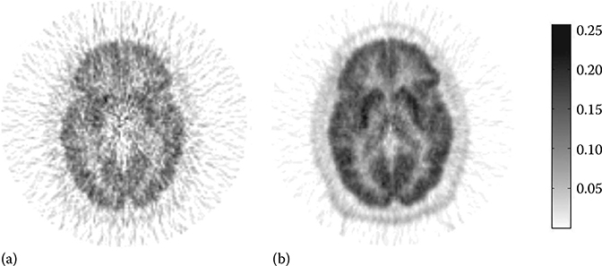
FIGURE 17.9
Parametric images of net accumulation rate K_in of [¹¹C]MeNTI using Gjedd-Patlak plot (a) and MLAIR2 (b). (Modified from Figure 17.6 in reference Kim, S.J. et al., J. Cereb. Blood Flow Metab. 2008, 28(12), 1965.)

Another multiple linear regression formula for tracers with reversible biding is MA2:

C_{t} (t) = P_{1} \int_{0}^{t} \int_{0}^{τ} C_{p} (s) d s d τ + P_{2} \int_{0}^{t} \int_{0}^{τ} C_{t} (s) d s d τ + P_{3} \int_{0}^{t} C_{t} (τ) d τ + P_{4} \int_{0}^{t} C_{p} (τ) d τ (17.52)

$C_{t} (t) = P_{1} \int_{0}^{t} \int_{0}^{τ} C_{p} (s) d s d τ + P_{2} \int_{0}^{t} \int_{0}^{τ} C_{t} (s) d s d τ + P_{3} \int_{0}^{t} C_{t} (τ) d τ + P_{4} \int_{0}^{t} C_{p} (τ) d τ (17.52)$

where the macro parameters P₁ ∼ P₄ are given by

\begin{matrix} P_{1} = k_{2} k_{4} V_{t} \\ P_{2} = - k_{2} k_{4} \\ P_{3} = - (k_{2} + k_{3} + k_{4}) \\ P_{4} = K_{1} \end{matrix} (17.53)

$\begin{matrix} P_{1} = k_{2} k_{4} V_{t} \\ P_{2} = - k_{2} k_{4} \\ P_{3} = - (k_{2} + k_{3} + k_{4}) \\ P_{4} = K_{1} \end{matrix} (17.53)$

The V_t can then be acquired using the following equation:

V_{t} = - \frac{P_{1}}{P_{2}} (17.54)

$V_{t} = - \frac{P_{1}}{P_{2}} (17.54)$

References

1. Aboagye E.O., Price P.M., Jones T.. In vivo pharmacokinetics and pharmacody-namics in drug development using positron-emission tomography. Drug Discov Today. 2001;6(6):293–302.

2. Fischman A.J., Alpert N.M., Rubin R.H.. Pharmacokinetic imaging: a noninvasive method for determining drug distribution and action. Clin Pharmacokinet. 2002;41(8):581–602.

3. Lowe V.J., Hoffman J.M., DeLong D.M., Patz E.F., Coleman R.E.. Semiquantitative and visual analysis of FDG-PET images in pulmonary abnormalities. J Nucl Med. 1994;35(11):1771–1776.

4. Cobelli C., Foster D., Toffolo G.. Tracer Kinetics in Biomedical Research: From Data to Model. New York: Kluwer Academic/Plenum Publishers; 2000.

5. Kety S.S.. The theory and application of the exchange inert gas at the lung and tissues. Pharmacol Rev. 1951;3:1–41.

6. Kety S.S.. Measurement of local blood flow by the exchange of an inert, diffusible substance. Methods Med Res. 1960;8:228–236.

7. Herrero P., Markham J., Myears D.W., Weiheimer C.J., Bergmann S.R.. Measurement of myocardial blood flow with positron emission tomography: correction for count spillover and partial volume effects. Math Comput Model. 1988;11:807–812.

8. Iida H., Rhodes C.G., de Silva R., Yamamoto Y., Araujo L.I., Maseri A., Myocardial tissue fraction-correction for partial volume effects and measure of tissue viability. J Nucl Med. 1991;32:2169–2175.

9. Phelps M.E., Huang S.C., Hoffman E.J., Selin C., Sokoloff L., Kuhl D.E.. Tomographic measurement of local cerebral glucose metabolic rate in humans with (F-18)2-fluoro-2-deoxy-D-glucose: validation of method. Ann Neurol. 1979;6(5):371–388.

10. Frost J.J., Douglass K.H., Mayberg H.S., Dannals R.F., Links J.M., Wilson A.A., Multicompartmental analysis of [¹¹C]-carfentanil binding to opiate receptors in humans measured by positron emission tomography. J Cereb Blood Flow Metab. 1989;9(3):398–409.

11. Gjedde A.. Calculation of cerebral glucose phosphorylation from brain uptake of glucose analogs in vivo: a re-examination. Brain Res. 1982;257(2):237–274.

12. Patlak C.S., Blasberg R.G.. Graphical evaluation of blood-to-brain transfer constants from multiple-time uptake data. Generalizations. J Cereb Blood Flow Metab. 1985;5(4):584–590.

13. Patlak C.S., Blasberg R.G., Fenstermacher J.D.. Graphical evaluation of blood-to-brain transfer constants from multiple-time uptake data. J Cereb Blood Flow Metab. 1983;3(1):1–7.

14. Schmidt K.C., Turkheimer F.E.. Kinetic modeling in positron emission tomography. Q J Nucl Med. 2002;46(1):70–85.

15. Ichise M., Meyer J.H., Yonekura Y.. An introduction to PET and SPECT neurore-ceptor quantification models. J Nucl Med. 2001;42(5):755–763.

16. Meyer J.H., Ichise M.. Modeling of receptor ligand data in PET and SPECT imaging: a review of major approaches. J Neuroimaging. 2001;11(1):30–39.

17. Wong D.F., Gjedde A., Wagner H.N.Jr. Quantification of neuroreceptors in the living human brain. I. Irreversible binding of ligands. J Cereb Blood Flow Metab. 1986;6(2):137–146.

18. Huang S.C., Barrio J.R., Phelps M.E.. Neuroreceptor assay with positron emission tomography: equilibrium versus dynamic approaches. J Cereb Blood Flow Metab. 1986;6(5):515–521.

19. Kuwabara H., Cumming P., Reith J., Leger G., Diksic M., Evans A.C., Human striatal L-dopa decarboxylase activity estimated in vivo using 6-[¹⁸F]fluoro-dopa and positron emission tomography: error analysis and application to normal subjects. J Cereb Blood Flow Metab. 1993;13(1):43–56.

20. Wong D.F., Yung B., Dannals R.F., Shaya E.K., Ravert H.T., Chen C.A., In vivo imaging of baboon and human dopamine transporters by positron emission tomography using [¹¹C]WIN 35,428. Synapse. 1993;15(2):130–142.

21. Hume S.P., Myers R., Bloomfield P.M., Opacka-Juffry J., Cremer J.E., Ahier R.G., Quantitation of carbon-11-labeled raclopride in rat striatum using positron emission tomography. Synapse. 1992;12(1):47–54.

22. Lammertsma A.A., Hume S.P.. Simplified reference tissue model for PET receptor studies. Neuroimage. 1996;4(3 Pt 1):153–158.

23. Logan J.. Graphical analysis of PET data applied to reversible and irreversible tracers. Nucl Med Biol. 2000;27(7):661–670.

24. Logan J., Fowler J.S., Volkow N.D., Wolf A.P., Dewey S.L., Schlyer D.J., Graphical analysis of reversible radioligand binding from time-activity measurements applied to [N-¹¹C-methyl]-(-)-cocaine PET studies in human subjects. J Cereb Blood Flow Metab. 1990;10(5):740–747.

25. Logan J., Fowler J.S., Volkow N.D., Wang G.J., Ding Y.S., Alexoff D.L.. Distribution volume ratios without blood sampling from graphical analysis of PET data. J Cereb Blood Flow Metab. 1996;16(5):834–840.

26. Cunningham V.J., Jones T.. Spectral analysis of dynamic PET studies. J Cereb Blood Flow Metab. 1993;13(1):15–23.

27. Meikle S.R., Matthews J.C., Brock C.S., Wells P., Harte R.J., Cunningham V.J., Pharmacokinetic assessment of novel anti-cancer drugs using spectral analysis and positron emission tomography: a feasibility study. Cancer Chemother Pharmacol. 1998;42(3):183–193.

28. Phelps M.E., Mazziotta J., Schelbert H.. Positron Emission Tomography and Autoradiography: Principle and Application for the Brain and Heart. New York: Raven Press; 1986.

29. Feng D., Huang S.-C., Wang Z., Ho D.. An unbiased parametric imaging algorithm for nonuniformly sampled biomedical system parameter estimation. IEEE Trans Med Imaging. 1996;15:512–518.

30. Feng D., Wang Z., Huang S.-C.. A study on statistically reliable and computationally efficient algorithms for generating local cerebral blood flow parametric images with positron emission tomography. IEEE Trans Med Imaging. 1993;12:182–188.

31. Bard Y.. Nonlinear Parameter Estimation. New York: Academic Press; 1974.

32. Marquardt D.W.. An algorithm for least squares estimations of nonlinear parameters. J Soc Ind Appl Math. 1963;11:431–441.

33. Lee J.S., Lee D.S., Ahn J.Y., Yeo J.S., Cheon G.J., Kim S.K., Park K.S., Chung J.K., Lee M.C.. Generation of parametric image of regional myocardial blood flow using H₂¹⁵O dynamic PET and a linear least-squares method. J Nucl Med. 2005;46(10):1687–1695.

34. Kim S.J., Lee J.S., Kim Y.K., Frost J., Wand G., McCaul M.E., Lee D.S.. Multiple linear analysis methods for the quantification of irreversibly binding radiotracers. J Cereb Blood Flow Metab. 2008;28(12):1965–1977.

35. Ichise M., Toyama H., Innis R.B., Carson R.E.. Strategies to improve neuroreceptor parameter estimation by linear regression analysis. J Cereb Blood Flow Metab. 2002;22(10):1271–1281.

..................Content has been hidden....................

You can't read the all page of ebook, please click here login for view all page.

Table of Contents for
17 Tracer Kinetic Analysis for PET and SPECT