8 Image Reconstruction Algorithms for X-Ray CT

Image reconstruction is to estimate a spatial distribution of some parameter inside an object from its projections, where projections are a set of measurements of the line integral values of the parameter. The parameter is a linear attenuation coefficient for transmission x-ray CT, while it is a radioactivity level in case of emission computed tomography (CT) such as single photon emission CT (SPECT) or positron emission tomography (PET).

Let f(x, y) be the two-dimensional (2-D) distribution of linear attenuation coefficients for monochromatic x-ray CT. Using the coordinate system described in Figure 8.1, projections p(θ, t), that is, line integrals of the object f(x, y) along a line L(θ, t) parameterized by (θ, t), are described as

Images

FIGURE 8.1
Parameters for parallel-beam projections.

p (θ, t) = \int ​ L (θ, t) f (x, y) d s = \int ​ \infty - \infty \int ​ \infty - \infty f (x, y) δ (x cos θ + y sin θ - t) d x d y = \int ​ \infty - \infty f (t θ ¯ + s θ ¯ ⊥) d s (8.1)

$\begin{matrix} p (θ, t) = \underset{L (θ, t)}{\int^{}} f (x, y) d s \\ = {\int^{}}_{\infty}^{- \infty} {\int^{}}_{\infty}^{- \infty} f (x, y) δ (x \cos θ + y \sin θ - t) d x d y \\ = {\int^{}}_{\infty}^{- \infty} f (t \underline{θ} + s {\underline{θ}}^{⊥}) d s \end{matrix} (8.1)$

where

δ(…) is the Dirac delta function

θ¯=(cosθ,sinθ) and θ¯⊥=(sinθ−cosθ) $\underline{θ} = (\cos θ, \sin θ) and {\underline{θ}}^{⊥} = (\sin θ - \cos θ)$ are two unit vectors which are orthogonal to each other

To transform a 2-D object f to its projections (or line integrals), p is called 2-D Radon transform. For reference, 3-D Radon data of a 3-D object f is plane integrals of the object.

The relationship of the intensity of two x-ray beams, one incident onto the object, I₀, and the other exiting from the object after the attenuation, I, can be expressed as

I = I 0 e x p ⎛ ⎝ ⎜ ⎜ ⎜ - \int ​ L (θ t) f (x, y) d s ⎞ ⎠ ⎟ ⎟ ⎟ (8.2)

$I = I_{0} e x p (- \underset{L (θ t)}{\int^{}} f (x, y) d s) (8.2)$

Images

FIGURE 8.2
A sinogram p(θ, t) of a chest phantom. |t_m| corresponds to the radial support of the phantom.

Thus, the projection can be obtained as

p (θ, t) = - ln (I I 0) (8.3)

$p (θ, t) = - \ln (\frac{I}{I_{0}}) (8.3)$

An example of projections is shown in Figure 8.2. Projection data are also called a sinogram, because when a point (x, y) is projected onto a line detector, the radial distance t of the projected point can be described by a trigonometric function with the angle θ, for example, t = t₀sinθ.

8.2 Central Slice Theorem (or Fourier Slice Theorem)

There are several ways to reconstruct the object f(x, y) from projections p(θ, t); however, the common foundation that relates the two functions is the central slice theorem (or Fourier slice theorem) (Figure 8.3).

\int ​ \infty - \infty p (θ, t) e x p (- 2 π i t ω) d t = F (ω cos θ, ω sin θ) = F p o l a r (θ, ω) (8.4)

${\int^{}}_{\infty}^{- \infty} p (θ, t) e x p (- 2 π i t ω) d t = F (ω \cos θ, ω \sin θ) = F_{p o l a r} (θ, ω) (8.4)$

Images

FIGURE 8.3
Central slice theorem (Fourier slice theorem).

where F(ω cos θ, ω sin θ) and F_polar(θ, ω) are the 2-D Fourier transform of the object f(x, y) in the Cartesian and polar coordinate systems, respectively. The proof is shown in the following.

\int ​ \infty - \infty p (θ, t) e x p (- 2 π i t ω) d t = \int ​ \infty - \infty ⎡ ⎣ ⎢ ⎢ ⎢ ⎢ \int ​ \infty - \infty \int ​ \infty - \infty f (x, y) δ (x cos θ + y sin θ - t) d x d y ⎤ ⎦ ⎥ ⎥ ⎥ ⎥ e x p (- 2 π i t ω) d t (∵ Equation 8 .1) = \int ​ \infty - \infty \int ​ \infty - \infty f (x, y) \int ​ \infty - \infty δ (x cos θ + y sin θ - t) e x p (- 2 π i t ω) d t] d x d y (Exchanging the order of integrals) = \int ​ \infty - \infty \int ​ \infty - \infty f (x, y) e x p (- 2 π i (x ω cos θ + y ω sin θ)) d x d y (∵ The property of delta function) = F (u, v) | u = ω cos θ, v = ω sin θ (8.5)

$\begin{array}{l} {\int^{}}_{\infty}^{- \infty} p (θ, t) e x p (- 2 π i t ω) d t \\ = {\int^{}}_{\infty}^{- \infty} [{\int^{}}_{\infty}^{- \infty} {\int^{}}_{\infty}^{- \infty} f (x, y) δ (x \cos θ + y \sin θ - t) d x d y] e x p (- 2 π i t ω) d t \\ (∵ Equation 8 .1) \\ = {\int^{}}_{\infty}^{- \infty} {\int^{}}_{\infty}^{- \infty} f (x, y) {\int^{}}_{\infty}^{- \infty} δ (x cos θ + y sin θ - t) e x p (- 2 π i t ω) d t] d x d y \\ (Exchanging the order of integrals) \\ = {\int^{}}_{\infty}^{- \infty} {\int^{}}_{\infty}^{- \infty} f (x, y) e x p (- 2 π i (x ω \cos θ + y ω \sin θ)) d x d y \\ (∵ The property of delta function) \\ = F (u, v) |_{u = ω \cos θ, v = ω \sin θ} \end{array} (8.5)$

The central slice theorem states as follows. The one-dimensional (1-D) Fourier transform of parallel-beam projections p(θ, t) at an angle θ is equal to the Fourier transform of the object f(x, y) along a line rotated by θ. Thus, once we obtain parallel-beam projections over 180° and calculate its Fourier transform, we can fill out the 2-D Fourier data space of the object, from which the object f(x, y) can be reconstructed by applying inverse 2-D Fourier transform. Note that this is the method mainly used in magnetic resonance imaging (MRI), where the Fourier space is called the K-space and the component data are directly measured. Thus, MR images can also be reconstructed using filtered backprojection or other algorithms we discuss later.

8.3 Filtered Backprojection (Parallel-Beam)

In the current medical x-ray CT systems, filtered backprojection (FBP) algorithms are the standard image reconstruction method while iterative methods (discussed later) are becoming options. In SPECT and PET scanners, both FBP and fully iterative image reconstruction methods may be equally utilized options. In this section, we derive the filtered backprojection formula from the central slice theorem.

We start with the object f as the inverse Fourier transform of 2-D Fourier transform spectrum F, and then convert it to the polar coordinate system.

f (x, y) = \int ​ \infty - \infty \int ​ \infty - \infty F (u, v) e x p (2 π i (x u + y v)) d u d v = \int ​ 2 π 0 \int ​ \infty 0 F p o l a r (θ, ω) e x p (2 π i ω (x cos θ + y s i n θ)) ω d ω d θ (8.6)

$\begin{matrix} f (x, y) = {\int^{}}_{\infty}^{- \infty} {\int^{}}_{\infty}^{- \infty} F (u, v) e x p (2 π i (x u + y v)) d u d v \\ = {\int^{}}_{2 π}^{0} {\int^{}}_{\infty}^{0} F_{p o l a r} (θ, ω) e x p (2 π i ω (x cos θ + y s i n θ)) ω d ω d θ \end{matrix} (8.6)$

where

u = ω cos θ

v = ω sin θ

du dv = ω dω dθ

Splitting the integration range into two and using symmetry, F(θ, ω) = F(θ + π, −ω), we get

f (x, y) = \int 0 π \int 0 \infty F p o l a r (θ, ω) exp (2 π i ω (x cos θ + y sin θ)) ω d ω d θ + \int π 2 π \int 0 \infty F p o l a r (θ, ω) exp (2 π i ω (x cos θ + y sin θ)) ω d ω d θ = \int 0 π \int - \infty \infty F p o l a r (θ, ω) exp (2 π i ω (x cos θ + y sin θ)) | ω | d ω d θ (8.7)

$\begin{matrix} f (x, y) = \int_{0}^{π} \int_{0}^{\infty} F_{p o l a r} (θ, ω) \exp (2 π i ω (x \cos θ + y \sin θ)) ω d ω d θ \\ + \int_{π}^{2 π} \int_{0}^{\infty} F_{p o l a r} (θ, ω) \exp (2 π i ω (x \cos θ + y \sin θ)) ω d ω d θ \\ = \int_{0}^{π} \int_{- \infty}^{\infty} F_{p o l a r} (θ, ω) \exp (2 π i ω (x \cos θ + y \sin θ)) | ω | d ω d θ \end{matrix} (8.7)$

Substituting the central slice theorem, Equation 8.4, into F_polar (θ, ω), we get

f (x, y) = \int ​ π 0 ⎧ ⎩ ⎨ ⎪ ⎪ ⎪ ⎪ ⎪ ⎪ \int ​ - \infty \infty ⎡ ⎣ ⎢ ⎢ ⎢ \int ​ - \infty \infty p (θ, t) e x p (- 2 π i t ω) d t ⎤ ⎦ ⎥ ⎥ ⎥ e x p (2 π i ω (x c o s θ + y s i n θ)) | ω | d ω ⎫ ⎭ ⎬ ⎪ ⎪ ⎪ ⎪ ⎪ ⎪ d θ = \int ​ 0 π p F (θ, t) d θ (8.8)

$\begin{matrix} f (x, y) = {\int^{}}_{π}^{0} {{\int^{}}_{- \infty}^{\infty} [{\int^{}}_{- \infty}^{\infty} p (θ, t) e x p (- 2 π i t ω) d t] e x p (2 π i ω (x c o s θ + y s i n θ)) | ω | d ω} d θ \\ = {\int^{}}_{0}^{π} p^{F} (θ, t) d θ \end{matrix} (8.8)$

where

p F (θ, t) = \int ​ - \infty \infty ⎡ ⎣ ⎢ ⎢ ⎢ \int ​ - \infty \infty p (θ, t) e x p (- 2 π i t ω) d t ⎤ ⎦ ⎥ ⎥ ⎥ e x p (2 π i ω (x c o s θ + y s i n θ)) | ω | d ω = \int ​ - \infty \infty p (θ, t) h R (t - t') d t' (8.9)

$\begin{matrix} p^{F} (θ, t) = {\int^{}}_{- \infty}^{\infty} [{\int^{}}_{- \infty}^{\infty} p (θ, t) e x p (- 2 π i t ω) d t] e x p (2 π i ω (x c o s θ + y s i n θ)) | ω | d ω \\ = {\int^{}}_{- \infty}^{\infty} p (θ, t) h_{R} (t - t') d t' \end{matrix} (8.9)$

and

h R (t) = \int - \infty \infty | ω | exp (2 π i ω t) d ω (8.10)

$h_{R} (t) = \int_{- \infty}^{\infty} | ω | \exp (2 π i ω t) d ω (8.10)$

Equations 8.8 through 8.10 show the following two steps for image reconstruction. First, parallel projections p are convolved with a ramp filter kernel h_R along the radial direction t. The convolution can be performed in the Fourier domain for more efficient computation. Then, the filtered projection p^F are “backprojected” onto the image space over [0, π) or 180°.

It is critical to have a clear mental picture of how images are reconstructed for investigating causes of artifacts, for example. To help readers understand the two steps in FBP intuitively, we show a result of computer simulation with a circular phantom with a diameter of 100 mm located at (0, 100 mm) in Figures 8.4 and 8.5. Figure 8.4 shows the projections p (a) and the filtered projections p^F (b), and the corresponding profiles at θ = π. Note that there are large negative values in p^F just outside t = (−t₀, t₀) where projections are nonzero, and the negative values rapidly increase toward zero.

Figure 8.5 visualizes the backprojection process over projection angle θ. It can be seen that the contour of the object becomes clearer or sharper as the angular range approaches to 180°. It can also be seen that outside the object, positive values backprojected from some angles and negative values from the other angles are cancelled out, resulting in zero. The image reconstruction is completed at 180°, and the same process is repeated from 180° to 360°.

Images

FIGURE 8.4
Projections p (a) and filtered projections p^F using Shepp–Logan filter (b) and the corresponding radial profiles at θ = π (c).

Images

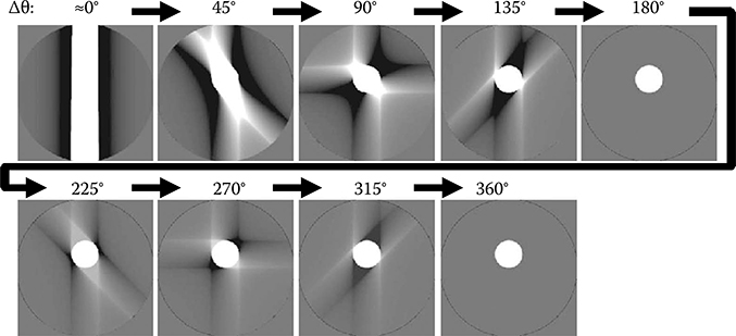
FIGURE 8.5
The process of an image being reconstructed by filtered backprojection of parallel-beam projections. Projections are in the north–south direction at θ = 0° and rotate in the counter-clockwise direction.

8.4 Filter Kernels

In reality, the ramp filter kernel |w| is truncated by the Nyquist frequency ω_Nq defined by the sampling condition

H R (ω) = {| ω | 0 | ω | \leq ω N q | ω | > ω N q (8.11)

$H_{R} (ω) = {\begin{matrix} | ω | & | ω | \leq ω_{N q} \\ 0 & | ω | > ω_{N q} \end{matrix} (8.11)$

This ramp filter provides the most accurate and the sharpest image of the object f(x, y) in a mathematical sense, correctly honoring all of the frequency components acquired by detectors. This filter, however, also provides the noisiest image at the presence of noise in projections. An analysis of frequency components of projections revealed that near the Nyquist frequency, there is less information from the object and more noise from quantum statistics. Shepp and Logan then proposed a modified ramp filter with an apodization window to suppress high-frequency components (i.e., “Shepp–Logan filter”) shown in Figure 8.6 [1,2]. This kernel suppresses the image noise, while minimizing the loss of the spatial resolution in clinical cases.

H R (ω) = ⎧ ⎩ ⎨ 2 ω N q π ∣ ∣ sin (π ω 2 ω N q) ∣ ∣ 0 | ω | \leq ω N q | ω | > ω N q (8.12)

$H_{R} (ω) = {\begin{matrix} \frac{2 ω_{N q}}{π} | \sin (\frac{π ω}{2 ω_{N q}}) | & | ω | \leq ω_{N q} \\ 0 & | ω | > ω_{N q} \end{matrix} (8.12)$

The Shepp–Logan filter is the standard one used for quality assurance tests in many x-ray CT scanners. But there are also other modified ramp filter kernels on CT scanners, which are specifically designed by enhancing and suppressing desirable frequency components for particular clinical applications such as body kernels, brain kernels, bone kernels, and lung kernels.

Images

FIGURE 8.6
The frequency response of filter kernels H_R(ω).

8.5 Filtered Backprojection (Fan-Beam)

Almost all of the x-ray CT scanners use x-ray beams divergent from the x-ray focal spot to acquire projections. Pin-hole and divergent collimators in SPECT scanners also use the divergent geometry. The geometry is called the fan-beam geometry for 2-D imaging and cone-beam geometry for 3-D imaging. Divergent beams require different FBP formula from parallel-beam geometry. In this section, we outline the FBP method for fan-beam geometry.

Fan-beam projections g(β, γ) are parameterized by a projection angle β, which is an angle that the source a makes with a reference axis, and a fan angle γ, which is a locally defined angle that rotates with the source a for the ray within a fan. Line integrals of an object f can be described using a unit vector Θ = (sin(β + γ), −cos(β + γ))

g (β, γ) = \int ​ 0 \infty f (a ¯ (β) + s Θ ¯ ¯ ¯) d s (8.13)

$g (β, γ) = {\int^{}}_{0}^{\infty} f (\underline{a} (β) + s \underline{Θ}) d s (8.13)$

Analytical methods to reconstruct images from fan-beam projections can be categorized into two groups. One is to rebin fan-beam projections into parallel-beam projections, which is called a fan-to-parallel-beam rebinning method, and the other is to reconstruct images directly from fan-beam projections, which is called a direct fan-beam FBP method. We will outline both of the methods in order.

Comparing Figure 8.7 with Figure 8.1, one may notice that the line L can be expressed using a different pair of parameters as L(β, γ) or L(θ, t). Thus, the x-ray beam along L in fan-beam projections and parallel-beam projections can be related as follows.

θ = β + γ, t = R sin γ (8.14)

$θ = β + γ, t = R \sin γ (8.14)$

where R is the distance from the origin to the source a = (−R sin β, R cos β). The line integral values obtained by the x-ray beam are identical; thus, one can map fan-beam projections g to parallel-beam projections p as

p (θ, t) = p (β + γ, R sin γ) = g (θ - sin - 1 (t R), sin - 1 (t R)) (8.15)

$p (θ, t) = p (β + γ, R \sin γ) = g (θ - \sin^{- 1} (\frac{t}{R}), \sin^{- 1} (\frac{t}{R})) (8.15)$

One can then employ the FBP method for parallel projections p to reconstruct an image f. This is the first, rebinning method.

Images

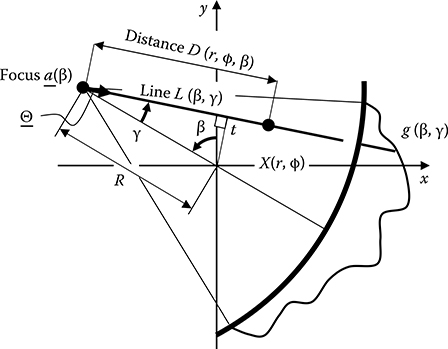
FIGURE 8.7
Parameters for fan-beam projections.

We now outline the second, direct FBP method from fan-beam projections. We start with describing the object f using the polar coordinate system (r, ϕ)

x = r cos ϕ, y = r sin ϕ (8.16)

$x = r \cos ϕ, y = r \sin ϕ (8.16)$

The FBP formula for parallel-beam geometry can then be rewritten as

f (r, ϕ) = 1 2 \int ​ 0 2 π ⎡ ⎣ ⎢ ⎢ ⎢ ⎢ \int ​ t m - t m p (θ, t) h R (r cos (θ - ϕ) - t) d t ⎤ ⎦ ⎥ ⎥ ⎥ ⎥ d θ = 1 2 \int ​ 0 2 π ⎡ ⎣ ⎢ ⎢ ⎢ \int ​ - γ m γ m p (β + γ, R sin γ) h R (r cos (β + γ - ϕ) - R sin γ) R cos γ d γ ⎤ ⎦ ⎥ ⎥ ⎥ d β [∵ d t = R cos γ d γ and Equations 8 .14 and 8 .15] (8.17)

$\begin{array}{l} f (r, ϕ) = \frac{1}{2} {\int^{}}_{0}^{2 π} [{\int^{}}_{t_{m}}^{- t_{m}} p (θ, t) h_{R} (r \cos (θ - ϕ) - t) d t] d θ \\ = \frac{1}{2} {\int^{}}_{0}^{2 π} [{\int^{}}_{- γ m}^{γ m} p (β + γ, R \sin γ) h_{R} (r \cos (β + γ - ϕ) - R \sin γ) R \cos γ d γ] d β \\ [∵ d t = R \cos γ d γ and Equations 8 .14 and 8 .15] \end{array} (8.17)$

where γm=sin−1(tm/R), tm $γ_{m} = \sin^{- 1} (t_{m} / R), t_{m}$ is the radius of the support of the object f. The backprojection range is extended from π to 2π, which is normalized by multiplying 1/2.

Now we make the argument of the kernel h_R shift-invariant. Let D be the distance from the focal spot to a point-of-interest X(r, ϕ) as shown in Figure 8.7, and γ′ be the fan angle of the ray that goes through X. Then from geometry, we have

D cos γ' = R + r sin (β - ϕ) (8.18)

$D \cos γ^{'} = R + r \sin (β - ϕ) (8.18)$

D sin γ' = r cos (β - ϕ) (8.19)

$D \sin γ^{'} = r \cos (β - ϕ) (8.19)$

and

D (r, ϕ, β) = (R + r sin (β - ϕ)) 2 + (r cos (β - ϕ)) 2 - - - - - - - - - - - - - - - - - - - - - - - - - - - - - \sqrt (8.20)

$D (r, ϕ, β) = \sqrt{{(R + r \sin (β - ϕ))}^{2} + {(r \cos (β - ϕ))}^{2}} (8.20)$

γ' = tan - 1 r cos ( β - ϕ ) R + r sin ( β - ϕ ) (8.21)

$γ^{'} = \tan^{- 1} \frac{r \cos (β - ϕ)}{R + r \sin (β - ϕ)} (8.21)$

By modifying D sin(γ′ − γ) using Equations 8.18 and 8.19, we get the argument of h_R in Equation 8.17 as follows.

D sin (γ' - γ) = D sin γ' cos γ - D cos γ' sin γ [∵ sin (a - b) = sin a cos b - cos a sin b] = r cos (β - ϕ) cos γ - (R + r sin (β - ϕ)) sin γ [∵ Equations 8 .18 and 8 .19] = r cos (β - ϕ + γ) - R sin γ [∵ cos (a + b) = cos a cos b - sin a sin b] (8.22)

$\begin{matrix} D \sin (γ^{'} - γ) = D \sin γ^{'} \cos γ - D \cos γ^{'} \sin γ \\ [∵ \sin (a - b) = \sin a \cos b - \cos a \sin b] \\ = r \cos (β - ϕ) \cos γ - (R + r \sin (β - ϕ)) \sin γ \\ [∵ Equations 8 .18 and 8 .19] \\ = r \cos (β - ϕ + γ) - R \sin γ \\ [∵ \cos (a + b) = \cos a \cos b - \sin a \sin b] \end{matrix} (8.22)$

Using Equations 8.15 and 8.22, Equation 8.17 can be modified to

f (γ, ϕ) = 1 2 \int - γ 2 π - γ ⎡ ⎣ ⎢ \int - γ m γ m g (β, γ) h R (D sin (γ' - γ)) R cos γ d γ ⎤ ⎦ ⎥ d β = 1 2 \int 0 2 π ⎡ ⎣ ⎢ \int - γ m γ m g (β, γ) h R (D sin (γ' - γ)) R cos γ d γ ⎤ ⎦ ⎥ d β (8.23)

$\begin{matrix} f (γ, ϕ) = \frac{1}{2} \int_{- γ}^{2 π - γ} [\int_{- γ_{m}}^{γ_{m}} g (β, γ) h_{R} (D \sin (γ^{'} - γ)) R \cos γ d γ] d β \\ = \frac{1}{2} \int_{0}^{2 π} [\int_{- γ_{m}}^{γ_{m}} g (β, γ) h_{R} (D \sin (γ^{'} - γ)) R \cos γ d γ] d β \end{matrix} (8.23)$

Here the periodicity of β over 2π is used to shift the integration range. Finally, we change the definition of the ramp filter kernel for parallel-beam projection, Equation 8.11, and obtain that for fan-beam projection

h g (γ) \equiv h R (D sin γ) = \int - \infty \infty | ω | exp (2 π i ω D sin γ) d ω = (γ D sin γ) 2 \int - \infty \infty | ω' | exp (2 π i ω' γ) d ω' = (γ D sin γ) 2 h R (γ) (8.24)

$\begin{matrix} h_{g} (γ) \equiv h_{R} (D \sin γ) \\ = \int_{- \infty}^{\infty} | ω | \exp (2 π i ω D \sin γ) d ω \\ = {(\frac{γ}{D \sin γ})}^{2} \int_{- \infty}^{\infty} | ω^{'} | \exp (2 π i ω^{'} γ) d ω^{'} \\ = {(\frac{γ}{D \sin γ})}^{2} h_{R} (γ) \end{matrix} (8.24)$

Equation 8.24 can be applied to other kernels such as Shepp–Logan filter.

Images

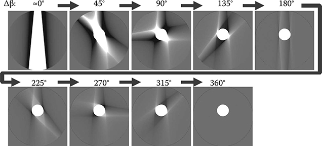
FIGURE 8.8
The process of an image being reconstructed by filtered backprojection of fan-beam projections. The focal spot is located at 12:00 at β = 0° and rotates in the counter-clock-wise direction.

In short, the FBP method that directly employs on fan-beam projections g is as follows:

f (γ, ϕ) = 1 2 \int 0 2 π 1 D 2 ( r , ϕ m , β ) \int - γ m γ m g (β, γ) h g (γ' - γ) R cos γ d γ d β (8.25)

$f (γ, ϕ) = \frac{1}{2} \int_{0}^{2 π} \frac{1}{D^{2} (r, ϕ m, β)} \int_{- γ_{m}}^{γ_{m}} g (β, γ) h_{g} (γ^{'} - γ) R \cos γ d γ d β (8.25)$

Similar to parallel-beam case, Equation 8.25 shows the following steps for image reconstruction. First, fan-beam projections g are weighted by cosγ. The weighted data are then convolved with a ramp filter kernel h_g with respect to the fan angle parameter γ. The filtered projections are backprojected onto the image space over [0, 2π) or 360° with a weight calculated by the inverse square distance from the focal spot to the voxel-of-interest, 1/D². Finally, the reconstructed image is scaled by R/2.

Similar to Figure 8.5 for parallel-beam projections, Figure 8.8 visualizes the backprojection process over projection angle β. It can be seen that the back-projected filtered data are spread from the focal spot side (on the north side when Δβ ≈ 0°) to the detector side (on the south side). Notice also that because of the divergent rays, the image reconstruction does not complete and artifact remains along the north–south direction when the backprojection is employed over 180°. It requires a full 360° for reconstruction to complete.

8.6 Redundancy in Projections

At the absence of scattered radiation, photon noise, and partial volume effect (and attenuation inside the object in case of SPECT and PET), projections of an object f can be calculated from line integrals of f along a ray alone, and independent of the direction of the x-ray beams. In other words, data are identical even if they are acquired when an x-ray focus and a detector swap the positions. One is called a primary ray, while the other is called a conjugate (or complementary) ray in CT community. The two rays can be related as follows (see Figure 8.9 for fan-beam projections):

Images

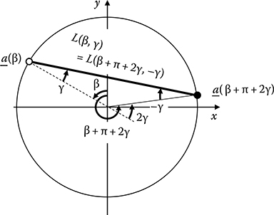
FIGURE 8.9
Conjugate (or complementary) rays in fan-beam projections.

p (θ, t) = p (θ + π, - t) [parallel-beam projections] (8.26)

$p (θ, t) = p (θ + π, - t) [parallel-beam projections] (8.26)$

g (β, γ) = g (β + π + 2 γ, - γ) [fan-beam projections] (8.27)

$g (β, γ) = g (β + π + 2 γ, - γ) [fan-beam projections] (8.27)$

Equations 8.26 and 8.27 are described using sinograms in Figure 8.10. Dashed lines indicate the primary rays at one projection angle, while solid lines indicate the corresponding conjugate rays. As shown in Equation 8.8, the angular range of projections that is necessary and sufficient for exact image reconstruction for parallel-beams is π regardless of the size of the object. The necessary angular range for fan-beams is π + 2γ_m (or 180° plus the full fan angle), where 2γ_m = 2sin⁻¹(t_m/R) is the full fan angle of the detector to image an object with a circular support with a radius of t_m.

Images

FIGURE 8.10
A primary ray at a projection angle (dashed line) and the corresponding conjugate ray (solid line) in parallel- (a) and fan-beam (b) projections. The heads and tails of the arrows indicate the corresponding order of the rays.

Images

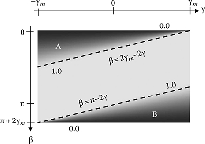
FIGURE 8.11
The redundancy weight w(β, γ) of the halfscan algorithm.

Among fan-beam projections over π + 2γ_m, a part of projection data (indicated by A and B in Figure 8.11) are acquired twice, while the rest of the data are obtained only once. Such unbalanced redundancy has to be normal-ized by applying a weighting function w(β, γ) to projections g prior to the convolution with h_g. With parallel-beam geometry or differentiated Hilbert transform approach, the weighting can be applied after filtering on a ray-basis or during the backprojection process on a voxel-basis.

Equation 8.25 is now generalized to

f (γ, ϕ) = \int 0 2 π 1 D 2 ( r , ϕ , β ) \int - γ m γ m w (β, γ) g (β, γ) h g (γ' - γ) R cos γ d γ d β (8.28)

$f (γ, ϕ) = \int_{0}^{2 π} \frac{1}{D^{2} (r, ϕ, β)} \int_{- γ_{m}}^{γ_{m}} w (β, γ) g (β, γ) h_{g} (γ^{'} - γ) R \cos γ d γ d β (8.28)$

Comparing Equation 8.25 with (8.28), the following observations can be made. When projections over 360° are used, all of the rays are measured exactly twice. Thus, w(β, γ) = 1/2 is applied to normalize the redundancy; and it is applied outside the integration because w is shift-invariant. Equation 8.25 is specifically called the fullscan.

The redundancy weighting function w(β, γ) has to satisfy the following two conditions [3]: it must be continuous and smooth (twice differentiable) with respect to γ; and a sum of weights for the primary and conjugate rays is equal to 1, thus

w (β, γ) + w (β + π + 2 γ, - γ) = 1 (8.29)

$w (β, γ) + w (β + π + 2 γ, - γ) = 1 (8.29)$

The w(β, γ) is also preferred to be continuous and smooth with respect to β, but it is not necessary. For example, the following function satisfies the two conditions and is called the halfscan algorithm [3,4] (Figure 8.11). Sometimes, it is loosely called short scan or partial scan as well.

w (β, γ) = 3 x 2 (β, γ) - 2 x 3 (β, γ) (8.30)

$w (β, γ) = 3 x^{2} (β, γ) - 2 x^{3} (β, γ) (8.30)$

x (β, γ) = ⎧ ⎩ ⎨ ⎪ ⎪ ⎪ ⎪ ⎪ ⎪ ⎪ ⎪ ⎪ ⎪ ⎪ ⎪ β 2 ( γ m + γ ) 1 π + 2 γ m - β 2 ( γ m - γ ) 0 [0 \leq β < 2 (γ m + γ)] [2 (γ m + γ) \leq β < π + 2 γ] [π + 2 γ + \leq β \leq π + 2 γ m] [otherwise] (8.31)

$x (β, γ) = {\begin{matrix} \frac{β}{2 (γ_{m} + γ)} & [0 \leq β < 2 (γ_{m} + γ)] \\ 1 & [2 (γ_{m} + γ) \leq β < π + 2 γ] \\ \frac{π + 2 γ_{m} - β}{2 (γ_{m} - γ)} & [π + 2 γ + \leq β \leq π + 2 γ_{m}] \\ 0 & [otherwise] \end{matrix} (8.31)$

Figure 8.12 shows fan-beam projections weighted by the halfscan weight and the filtered weighted projections. Note that projections near β = 0° and π + 2γ_m are lightly weighted and their contribution to image are decreased. Figure 8.13 shows the backprojection progresses of the halfscan algorithm. It can be seen that an image free from artifacts is reconstructed at Δβ = 225° (180° plus full fan angle).

This redundancy-based approach can be further generalized for projections acquired over multiple (N > 1) rotations as follows, which can be applied to various cases such as electrocardiogram-gated cardiac image reconstruction, compensation of detector defects, and image reconstruction of a large field of view with asymmetric detectors.

f (r, ϕ) = \sum n = 0 N - 1 \int 0 2 π 1 D 2 ( r , ϕ , β ) \int - γ m γ m w (β + 2 π n, γ) g (β + 2 π n, γ) h g (γ' - γ) R cos γ d γ d β (8.32)

$f (r, ϕ) = \sum_{n = 0}^{N - 1} \int_{0}^{2 π} \frac{1}{D^{2} (r, ϕ, β)} \int_{- γ_{m}}^{γ_{m}} w (β + 2 π n, γ) g (β + 2 π n, γ) h_{g} (γ^{'} - γ) R \cos γ d γ d β (8.32)$

\sum n = 0 N - 1 (w (β + 2 π n, γ) + w (β + (2 n + 1) π + 2 γ, - γ)) = 1 (8.33)

$\sum_{n = 0}^{N - 1} (w (β + 2 π n, γ) + w (β + (2 n + 1) π + 2 γ, - γ)) = 1 (8.33)$

Images

FIGURE 8.12
Weighted projections using the halfscan weight (a) and the weighted filtered projections using Shepp–Logan filter (b) of the circular phantom.

Images

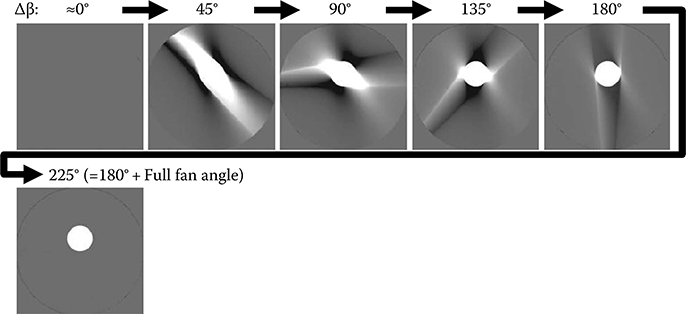
FIGURE 8.13
The process of an image being reconstructed by weighted filtered backprojection of fan-beam projections using the halfscan weight.

8.7 Cone-Beam Reconstruction

Diagnostic multidetector-row CT (MDCT) and flat-panel detector-based C-arm cone-beam CT (CBCT) acquire cone-beam projections, which are divergent with respect to z-axis (or the longitudinal direction of the object) as well as xy-axes. The angle of rays measured from the xy-plane is called the cone angle. When a number of detector rows in MDCT is small (e.g., <10 rows), such divergence is ignored and projections are treated as stacked fan-beam projections. This approach is similar to the single-slice rebinning approach used in PET and provides good image quality with no blurring along z-axis when the cone angle is small.

When the number of detector rows is large (thus the cone angle is large), however, image reconstruction algorithms have to take into account such divergence to minimize the cone angle artifacts we will discuss later. There are two methods most frequently used in CT scanners, which are extensions of the two FBP methods outlined in the fan-beam FBP section: Feldkamp algorithm [5] and cone-to-parallel fan-beam rebinning method [6–8]. The same methods can be employed with various scan modes such as an axial scan, a step-and-shoot scan, a helical or spiral scan, and a shuttle scan with appropriate redundancy weights.

The first method, Feldkamp algorithm or FDK algorithm, is an extension of the direct fan-beam FBP method and performs the following three steps which are very similar to the steps in the direct fan-beam FBP method. First, cone-beam projections g(β, γ, α) are weighted by w(β, γ, α)cosαcosγ, where α is the cone-angle and γ is the fan-angle, respectively, of the ray and w is the redundancy weight. Next, the weighted projections are convolved with a ramp filter kernel h_g, which is identical to the one designed for fan-beam, with respect to the fan angle parameter γ along the detector-row direction. Finally, the filtered projections are backprojected to voxels along the path the ray is acquired with the same weight used in fan-beam case, that is, an inverse square distance of the focal spot to the voxel-of-interest projected onto xy-plane (Figure 8.14).

f (r, ϕ, z) = \int 0 2 π 1 D 2 ( r , ϕ , β ) \int - γ m γ m w (β, γ, α) g (β, γ, α) h g (γ' - γ) R cos α cos γ d γ d β (8.34)

$f (r, ϕ, z) = \int_{0}^{2 π} \frac{1}{D^{2} (r, ϕ, β)} \int_{- γ_{m}}^{γ_{m}} w (β, γ, α) g (β, γ, α) h_{g} (γ^{'} - γ) R \cos α \cos γ d γ d β (8.34)$

It can be seen that the major differences from direct fan-beam FBP method are the weighting by cosα, which compensates for increased path-lengths due to the cone-angle α and the cone-beam backprojection. Although this method had been considered empirical and inaccurate, later studies showed that Feldkamp algorithm is equivalent to the exact inverse 3-D Radon transform when employed with a flat-panel detector, an appropriate scan orbit, and redundancy weights [9,10]. A derivative of Feldkamp method is a hybrid filtering approach, which approximately replaces a ramp filtering by a combination of a ramp filtering and a differentiation step and Hilbert filtering, followed by cone-beam backprojection with an inverse distance weight [11].

Images

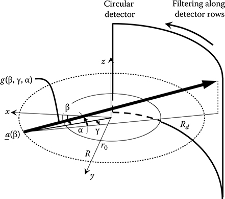
FIGURE 8.14
Cone-beam projections are filtered along detector rows and cone-beam backprojected along the path the x-ray beams are acquired.

The second method, cone-to-parallel fan-beam rebinning method, is an extension of the fan-to-parallel-beam rebinning method shown in Equations 8.14 and 8.15 and performs the following four steps. First, the fan-to-parallel-beam rebinning outlined previously is applied independently to each of cone-beam projections g(β, γ, α) acquired by the same detector row α as described in Equation 8.35 and Figure 8.15. This process is called cone-to-parallel fan-beam rebinning. Note that the projections from different detector rows are not mixed in this process; thus, the rebinned data p(θ, t, α) maintain the divergence of beams along z-axis, while the projection of p onto the xy-plane are parallel-beams parameterized by (θ, t). Next, the rebinned data acquired by the same detector row α are convolved with the ramp filter kernel h_R, which is identical to the one designed for parallel-beam, with respect to the radial parameter t. Finally, the filtered data are backprojected to voxels along the path the ray is acquired while being weighted by w(θ, x, y, z) cos α. Note that unlike direct fan- or cone-beam FBP methods, the redundancy weight optimized for each voxel can be applied during the backpro-jection process if desired. Because the shape of the rebinned data p(θ, t, α) looks like a wedge, this algorithm is sometimes called Wedge algorithm.

p (θ, t, α) = p (β + γ, R sin γ, α) = g (θ - sin - 1 (t R), sin - 1 (t R), α) (8.35)

$p (θ, t, α) = p (β + γ, R \sin γ, α) = g (θ - \sin^{- 1} (\frac{t}{R}), \sin^{- 1} (\frac{t}{R}), α) (8.35)$

Images

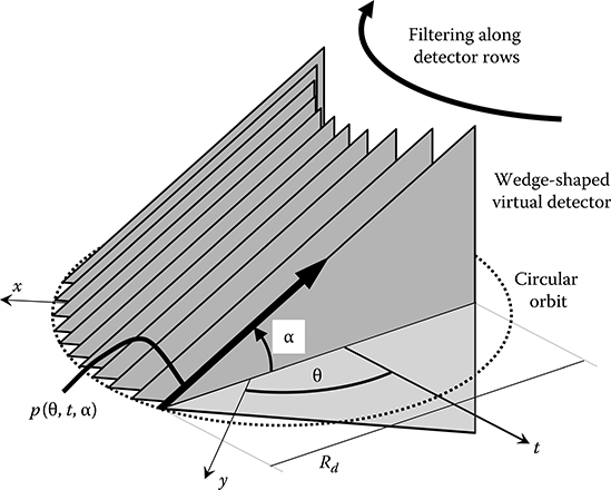
FIGURE 8.15
Cone-to-parallel fan-beam rebinning method. A part of cone-beam projections acquired at a series of focal spot positions are used to select projections that are parallel in the xy-plane, but divergent in z-axis. The rebinned projections are then filtered along the detector rows.

f (x, y, z) = \int 0 π w (θ, x, y, z) \int - \infty \infty p (θ, t, α) h R (t - t') cos α d t' d θ (8.36)

$f (x, y, z) = \int_{0}^{π} w (θ, x, y, z) \int_{- \infty}^{\infty} p (θ, t, α) h_{R} (t - t^{'}) \cos α d t^{'} d θ (8.36)$

The above two cone-beam image reconstruction methods significantly improve the image artifacts compared with the single-slice rebinning approach. The image quality is sufficient with the full cone angle up to ∼5° to 10°. When the total cone angle is larger, however, there is a risk of shading artifacts and blurred edges near objects with high contrast and with a rapid change of shape in z-axis (see Figure 8.16). These are called cone-beam artifacts.

The cone-beam artifacts are generated because an axial scan along a circular orbit will not provide a complete 3-D Radon data necessary to reconstruct an exact 3-D image [5,12] (Figure 8.17). The halfscan weight designed to normalize the redundancy of 2-D Radon data may be applied for a better temporal resolution, for example. Such weights do not take into account the redundancy of 3-D Radon data correctly, and thus further degrades the image quality. A redundancy weight that balances the redundancy and the amount of the 3-D Radon data and the temporal resolution provides better image quality [12].

Images

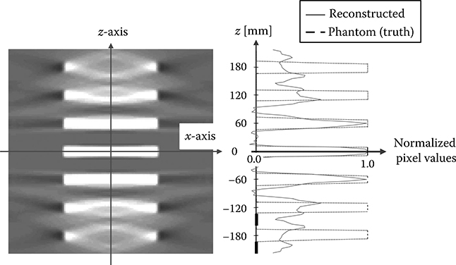
FIGURE 8.16
Cone-beam artifacts in a coronal view. A phantom with stacked disks was scanned by a circular scan at z = 0 mm, and the coronal image at y = 0 was reconstructed by Feldkamp algorithm. The focus-to-isocenter distance was 600 mm. Images near the scan plane was sharp and accurate, while images become blurry and inaccurate with shading artifacts away from the scan plane due to the effect of cone-angle.

Images

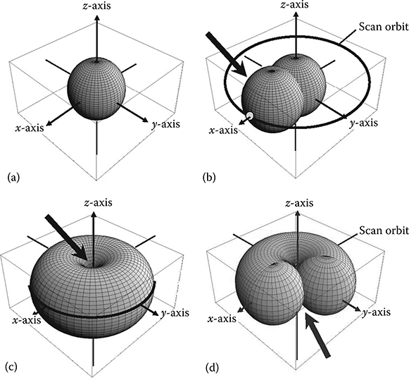
FIGURE 8.17
The necessary and obtained 3-D-Radon data (plane integrals) in 3-D-Radon space. (a) The necessary 3-D-Radon data for reconstructing an object within a ball whose radius is r₀. (b) The obtained 3-D-Radon data by a focus at β, can be described by the “surface” of the ball (arrow), whose diameter is defined by the locations of the focus and the origin. (c) Obtained 3-D-Radon data with one rotation are the surface and inside of the donut region. Comparing the obtained with the necessary 3-D Radon data (a), it can be seen that “the core of the apple” indicated by the arrow is not acquired. This is the reason of cone-beam shading artifacts away from z = 0 plane. (d) Fullscan Feldkamp algorithm uses the 3-D Radon data shown in (c) completely, while nonzero 3-D-Radon data used by with halfscan Feldkamp algorithm shows reduced utilization of 3-D Radon data, throwing away a part of the acquired 3-D Radon data (arrow). (From Taguchi, K., Medical Physics, 30, 640, 2003.)

8.8 Iterative Reconstruction Methods

8.8.1 Iterative Image Reconstruction Methods for SPECT and PET

Iterative image reconstruction (IR) methods have been investigated for many years in research community, and are now implemented and used on SPECT and PET scanners as frequently as FBP methods. The IR methods estimate the image of the object by minimizing a cost function that is defined based on a difference between the measured and the calculated projections incorporating various nonlinear physics factors such as the photon noise, the attenuation and scattering of emitted photons inside the object, and the geometrical efficiency and aperture of detectors and collimators [13]. We will outline the concept of the IR methods in this section.

When the projection process is linear, it can be described by a matrix H, which can then relate the object f and its cone-beam projection g as

g = H f (8.37)

$g = H f (8.37)$

The image reconstruction is then to obtain f from g. The FBP is an analytical, one-time method to apply the inverse of H, H⁻¹, to g. There are numerical, iterative approaches such as the algebraic reconstruction technique (ART) and simultaneous ART (SART) that use the transpose of H, H^T, and incrementally update the estimate of f to decrease the difference between the measured projection g˜ $\tilde{g}$ and the estimated projection g = Hf^(k) from the current estimate f^(k) at the k-th iteration. A calculation of g requires a forward projection operation Hf^(k), while the update of the estimate is performed using the difference of the two projections as

f (k + 1) = f (k) + λ w H H T (g ˜ - g) (8.38)

$f^{(k + 1)} = f^{(k)} + λ w_{H} H^{T} (\tilde{g} - g) (8.38)$

where

H^T is the transpose of H, that is, a backprojection operation

w_H is a weighting coefficient for the contribution of voxels to a ray

λ is a parameter to control the speed of convergence

Note that one forward- and one backprojection operation is performed for one iteration process, which are required to accurately model the relation of f to g.

When the projection process is nonlinear due to the factors listed earlier, the relationship can be described as

g ~ Poisson (H D A f + g s) (8.39)

$g ~ Poisson (H_{D A} f + g s) (8.39)$

where

H_DA is a modified system matrix incorporating the geometrical efficiency and detector apertures and the attenuation

g_S is measurements due to scattered photons

The IR methods try to minimize the cost function, for example,

f ˆ = arg min f L L (g ˜ | f) + ρ R (f) (8.40)

$\hat{f} = \arg \min_{f} L L (\tilde{g} | f) + ρ ℛ (f) (8.40)$

where

LL(g˜|f) $L L (\tilde{g} | f)$ is a negative log-likelihood of g˜ $\tilde{g}$ given f

R(f) $ℛ (f)$ is a roughness penalty or a priori knowledge of f (e.g., log of a Gibbs prior distribution)

ρ is a parameter that balances the effect of the two terms

The update equation is more complex than ART; however, it uses one forward- and one backprojection operation per iteration.

Considering that FBP only uses one backprojection operation to reconstruct an image, performing N_IR iterations of IR methods in general is roughly (2N_IR − 1) times as computationally expensive as FBP. In return, IR methods often provide more accurate and less noisy images than FBP does, thanks to accurate modeling of the nonlinear factors mentioned earlier.

8.8.2 Iterative Methods for CT

Most of iterative methods lately implemented to x-ray CT scanners seem to be different from the IR methods used in SPECT and PET. Although details are not published, some of the iterative methods (IM) may merely be an iterative image processing method, but loosely called an iterative image reconstruction method for better marketing purposes.

The current CT scanners never employ FBP alone. They perform various types of adaptive (sometimes iterative) methods to correct and process projection data prior to FBP, employ FBP, followed by various adaptive (sometimes iterative) methods on the image data to enhance the image quality. The most important nonlinear effect in x-ray CT is beam hardening effects (BHE). The BHE due to soft tissues is corrected during the adaptive pre-FBP correction process, while the BHE due to bones or contrast agents is corrected in an iterative fashion with one or a few iterations, using forward- and back-projections [14]. The adaptive post-FBP processes include an adaptive edge preserving noise reduction filtering.

The IM replaces a part of the adaptive pre-FBP processes on projections by iterative methods using statistical properties of projections and a part of the adaptive post-FBP process on image data by iterative methods using a priori knowledge and the statistical properties of the image. The iterative methods seem more aggressive than the current adaptive methods designed for similar purposes.

In contrast, true IR methods for CT may consist of a part of the adaptive pre-FBP processes, iterative image reconstruction using forward- and back-projection to iteratively estimate the image [15,16], and a part of the adaptive post-FBP processes. It is not clear at this moment which algorithms on CT scanners are IM and which are IR.

As it can be seen, both the IM and the current adaptive schemes are similar, sandwiching FBP by pre- and post-processes. If the IM models the forward imaging process, various nonlinear effects, and properties of images better than the adaptive pre- and post-FBP processes, the IM methods can provide images superior to the current CT images. The IM also has a risk of creating unrealistic images if inappropriate priors are used. The computational costs of IM and FBP may be comparable, because the most expensive step may remain the FBP process. IR methods can outperform either of the two methods, if nonlinear factors that can only be modeled in forward- and backprojection process are significant.

8.9 Other Class of Algorithms

Recently, other novel image reconstruction methods have developed. A Hilbert transform-based FBP (super short scan) method allows for reconstructing a part of the image from fan-beam projections over less than 180° [17,18]. When a detector is not large enough to cover the entire object, the trans-axial truncation caused strong biases and artifacts with the standard FBP method. But employing differentiated backprojection followed by inverse Hilbert transform on the image (DBP, BPF, or DBPF) accurately reconstructs an imaged region from such truncated projections.

Compressive sensing allows for exact reconstruction even from an extremely fewer number of projections that does not satisfy Nyquist–Shannon sampling theorem, when the object pixel values are piecewise constant [19–21]. The application of this method to CB-CT may be more appropriate than to diagnostic CT, because CB-CT always uses pulsed x-rays; thus, it can intentionally decrease the number of projections for some merits and use the compressive sensing technique to overcome the sampling problem. In contrast, x-rays are always on during the scan in diagnostic x-ray CT systems and it is difficult to pulse x-rays, because the time duration per projection is as short as 100–300 μs.

8.10 Artifacts (z-Aliasing, Cone-Angle, Scatter, Halfscan)

We outline a few artifacts that are unique to x-ray CT and related to image reconstruction.

8.10.1 Aliasing Artifacts or “Windmill” Artifacts

Windmill artifacts are black-and-white spokes (Figure 8.18) centering at high-contrast structures, which change the shape rapidly in z-axis such as bones at the base of skull, air pockets in intestines. The windmill artifacts rotate when we page through images along z-axis, which is why they are called windmill artifacts.

The windmill artifacts are caused by the aliasing along z-axis—the Nyquist frequency defined by a sampling pitch along z-axis (which is often defined by the interval of detector rows in MDCT) does not satisfy the maximum frequency component of the structure-of-interest [22,23]. It has been shown that extending the polar artifacts to the scan orbit, they cross at projection angles where detector rows that correspond to the image voxel-of-interest switch over [22,23].

There are a few methods to mitigate the problem. First one is to utilize a helical pitch that interlaces the sampling positions of primary and conjugate rays in z-axis, thus decreasing the sampling pitch. The concept is similar to quarter offset detector alignment in xy-plane and can be applicable to both fan- [22,24] and cone-beam backprojection [25]. The second one is to employ cone-beam backprojection from a virtual focal spot position that is slightly offset from the actual position. This simple scheme suppresses the aliased frequency components while minimizing the loss of the original frequency components [26]. The third one is to alternate between two z-positions of the x-ray focal spot, acquiring two samples per detector row. This scheme called z flying focal spot or zFFS doubles the number of samples in the z-axis and decreases the sampling interval to the half at the iso-center [27].

Images

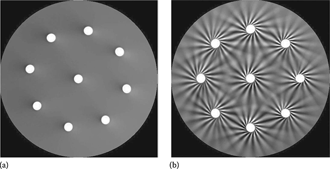
FIGURE 8.18
Cone-beam artifacts (a) and windmill artifacts (b). The phantom consists of nine balls with a diameter of 20 mm. A helical scan was performed by a MDCT with a beam width of 32 mm using a helical pitch of 1.0. Images at the edge of the ball with a thickness of 2.5 mm were reconstructed. The only difference between the two images was the configuration of the detector rows: 160 rows × 0.2 mm/row (a) and 16 rows × 2.0 mm/row (b). (From Silver, M. D. et al., SPIE Medical Imaging: Image Processing, San Diego, CA, 5032, 1918, 2003.)

8.10.2 Cone-beam Artifacts

Cone-beam artifacts are broad artifacts in either shading or brightening spread on both sides of structures with a rapid change of shape along z-axis (see Figure 8.16).

There are two methods to mitigate the problem. First one is to use a scan mode (more specifically, a trajectory of the x-ray focal spot) that acquires more 3-D Radon data. For example, choose a helical scan over an axial scan when possible. The second one is to perform an image reconstruction algorithm and a redundancy weight that use more 3-D Radon data and are mathematically exact (or better approximate the exact solutions). An example of the redundancy weights will be discussed in the next section.

8.10.3 Halfscan Artifacts

The following phenomena are called halfscan artifacts which have been discovered relatively recently [12,28]: a larger degree of shading and brightening and a shift (or bias) of overall pixel values compared with the fullscan case, and changes of the these problems as a function of the projection angle that corresponds to the center of the halfscan range. Investigations on the artifacts are likely to continue.

Several causes may result in the artifacts; however, the main cause is considered to be a mismatch between the 3-D path of the primary ray and that of the conjugate ray, both of which cross a voxel-of-interest from the opposite direction (see Figure 8.19). The halfscan weight, derived to normalize the redundancy of 2-D Radon data, does not normalize the redundancy of 3-D Radon data. Therefore, when halfscan weight is applied to cone-beam projections, it eliminates a part of 3-D Radon data acquired by a circular, axial scan (which already is not sufficient to reconstruct exact images) (see Figure 8.17 and Reference [12] for more details). The mismatch of paths also results in discrepancies between the two rays in terms of the scattered radiation and beam hardening effects. This is the reason why image artifacts are stronger in the halfscan case than in the fullscan case and why the strengths and ranges of artifacts depend on the halfscan angle.

The other causes of halfscan artifacts include the mechanical vibration of the gantry, the effect of object motion, and the cross-scatter. The strength and direction of motion artifacts with deforming objects, such as heart, depend on the halfscan angle [29]. In dual-source CT systems, where two sets (A and B) of an x-ray tube and a detector are aligned almost perpendicularly, x-ray beams generated by one x-ray tube (A) may be scattered by the object and be detected by the other detector (B) and vice versa. The cross-scatter may leave a bias and noise even after a correction, both of which may change with the halfscan angle.

Images

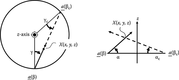
FIGURE 8.19
The paths of a primary ray and the corresponding conjugate ray do not match in cone-beam projections.

References

1. L. A. Shepp and B. F. Logan, The Fourier reconstruction of a head section, IEEE Transactions on Nuclear Science, NS-21, 21–43, 1974.

2. A. C. Kak and M. Slaney, Principles of Computerized Tomographic Imaging. New York: IEEE Press, 1987.

3. D. L. Parker, Optimal short scan convolution reconstruction for fanbeam CT, Medical Physics, 9, 254–257, 1982.

4. C. R. Crawford and K. F. King, Computed tomography scanning with simultaneous patient translation, Medical Physics, 17, 967–982, 1990.

5. L. A. Feldkamp, L. C. Davis, and J. W. Kress, Practical cone-beam algorithm, Journal of the Optical Society of America A, 1, 612–619, June 1984.

6. M. Grass, T. Kohler, and R. Proksa, 3D cone-beam CT reconstruction for circular trajectories, Physics in Medicine and Biology, 45, 329–347, 2000.

7. M. Grass, T. Kohler, and R. Proksa, Angular weighted hybrid cone-beam CT reconstruction for circular trajectories, Physics in Medicine and Biology, 46, 1595–1610, 2001.

8. H. K. Tuy, Three-dimensional image reconstruction for helical partial cone-beam scanners, Presented at the 5th International Conference on Fully Three-Dimensional Reconstruction in Radiology and Nuclear Medicine, Egmond Ann Zee, the Netherlands, 1999.

9. H. Kudo and T. Saito, Derivation and implementation of a cone-beam reconstruction algorithm for nonplanar orbits, IEEE Transactions on Medical Imaging, 13, 196–211, 1994.

10. M. Defrise and R. Clack, A cone-beam reconstruction algorithm using shift-variant filtering and cone-beam backprojection, IEEE Transactions on Medical Imaging, 13, 186–195, 1994.

11. A. A. Zamyatin, K. Taguchi, and M. D. Silver, Practical hybrid convolution algorithm for helical CT reconstruction, IEEE Transactions on Nuclear Science, 53, 167–174, 2006.

12. K. Taguchi, Temporal resolution and the evaluation of candidate algorithms for four-dimensional CT, Medical Physics, 30, 640–650, 2003.

13. K. Lange and R. Carson, EM reconstruction algorithms for emission and transmission tomography, Journal of Computer Assisted Tomography, 8, 306–316, 1984.

14. J. M. Meagher, C. D. MoteJr., and H. B. Skinner, CT image correction for beam hardening using simulated projection data, IEEE Transactions on Nuclear Science, 37, 1520–1524, 1990.

15. I. A. Elbakri and J. A. Fessler, Statistical image reconstruction for polyenergetic x-ray computed tomography, IEEE Transactions on Medical Imaging, 21, 89–99, 2002.

16. Y. Zhou, J.-B. Thibault, C. A. Bouman, K. D. Sauer, and J. Hsieh, Fast model-based x-ray CT reconstruction using spatially nonhomogeneous ICD optimization, IEEE Transactions on Image Processing, 20, 161–175, 2011.

17. F. Noo, M. Defrise, R. Clackdoyle, and H. Kudo, Image reconstruction from fan-beam projections on less than a short scan, Physics in Medicine and Biology, 47, 2525–2546, 2002.

18. H. Kudo, T. Rodet, F. Noo, and M. Defrise, Exact and approximate algorithms for helical cone-beam CT, Physics in Medicine and Biology, 49, 2913–2931, 2004.

19. E. J. Candes, J. Romberg, and T. Tao, Robust uncertainty principles: exact signal reconstruction from highly incomplete frequency information, IEEE Transactions on Information Theory, 52, 489–509, 2006.

20. D. L. Donoho, Compressed sensing, IEEE Transactions on Information Theory, 52, 1289–1306, 2006.

21. E. Y. Sidky, C.-M. Kao, and X. Pan, Accurate image reconstruction from few-views and limited-angle data in divergent-beam CT, Journal of X-Ray Science and Technology, 14, 119–139, 2006.

22. K. Taguchi, H. Aradate, Y. Saito, I. Zmora, K. S. Han, and M. D. Silver, The cause of the artifact in 4-slice helical computed tomography, Medical Physics, 31, 2033–2037, 2004.

23. M. D. Silver, K. Taguchi, I. A. Hein, B. S. Chiang, M. Kazama, and I. Mori, Windmill artifact in multi-slice helical CT, in SPIE Medical Imaging: Image Processing, San Diego, CA, 5032, 1918–1927, 2003.

24. K. Taguchi and H. Aradate, Algorithm for image reconstruction in multi-slice helical CT, Medical Physics, 25, 550–561, 1998.

25. J. Hsieh, X. Tang, J.-B. Thibault, C. Shaughnessy, R. A. Nilsen, and E. Williams, Conjugate cone-beam reconstruction algorithm, Optical Engineering, 46, 067001–067010, 2007.

26. I. Mori, Antialiasing backprojection for helical MDCT, Medical Physics, 35, 1065–1077, 2008.

27. T. G. Flohr, K. Stierstorfer, S. Ulzheimer, H. Bruder, A. N. Primak, and C. H. McCollough, Image reconstruction and image quality evaluation for a 64-slice CT scanner with z-flying focal spot, Medical Physics, 32, 2536–2547, 2005.

28. A. N. Primak, Y. Dong, O. P. Dzyubak, S. M. Jorgensen, C. H. McCollough, and E. L. Ritman, A technical solution to avoid partial scan artifacts in cardiac MDCT, Medical Physics, 34, 4726–4737, 2007.

29. K. Taguchi and A. Khaled, Artifacts in cardiac computed tomographic images, Journal of the American College of Radiology, 6, 590–593, 2009.

..................Content has been hidden....................

You can't read the all page of ebook, please click here login for view all page.

Table of Contents for
8 Image Reconstruction Algorithms for X-Ray CT