Chapter 8
Polymers: Solutions, Blends, Membranes, and Gels

Polymer solutions are liquid mixtures wherein the molecules of at least one component are very much larger than those of the other components. For many linear and branched polymers, liquid solvents are available that dissolve the polymer completely to form a homogeneous solution. However, cross-linked polymers (i.e. networks) only swell when in contact with a compatible liquid solvent. Swelling also occurs when polymeric materials are exposed to solvent vapors or gases that can be absorbed by the polymer.

A polymer blend is a mixture containing two or more polymers and, perhaps, an additional component to enhance polymer compatibility.

The phase behavior of polymer solutions and the swelling of polymers play important roles in polymer processing and in at least some applications, primarily because many polymers are produced in solution and therefore the final polymer product may contain some residual solvent. The physical properties of polymers are affected by the amount and type of the low-molecular-weight components they contain. A frequent technical problem is to remove essentially all the low-molecular-weight components; a common procedure is to volatilize them and this removal process is often called polymer devolatilization. Total removal of solvent is particularly important for polymeric films used in packaging foods or Pharmaceuticals. In other cases, the important technical issue is how much and how fast liquid solvent or vapor or gas is absorbed by a polymer. Processes where sorption behavior is important are, for example, the separation of gaseous and liquid mixtures using nonporous polymeric membranes or the use of supercritical fluids as swelling agents for impregnating polymers with chemical additives (e.g. pigments for color) and, conversely, for extracting low-molecular-weight components from polymeric materials. Qualitative and quantitative description of these processes requires first, knowledge of phase behavior and solubility (equilibrium properties)¹ and second, of diffusivity (transport property). Equilibrium properties must be known to provide a meaningful description of the driving force for a diffusion process.

¹ Methods for calculating equilibrium properties of polymer solutions and a database are presented by R. P. Danner and M. S. High, 1993, Handbook of Polymer Solution Thermodynamics, New York: A.I.Ch.E.

This chapter presents an introduction to the phase behavior of polymer-solvent solutions and polymer blends. We also briefly address the solubility and diffusivity of low-molecular-weight components in polymeric materials (e.g. membranes) and the unique phase behavior of polymeric gels. However, before these particular topics are addressed, we summarize some special properties of polymers.

8.1 Properties of Polymers

Polymers are large, chain-like molecules composed of many (Greek: poly-) structural repeating units, or “mers” (Greek: meros meaning part), connected by chemical bonds. These units may be arranged in a variety of ways resulting in various types of molecules with chain-like structure. The simplest is a linear polymer where the units are connected to each other in a linear sequence forming a long chain. An alternative to a linear polymer is a branched polymer. The branches can be long or short. When branches of different polymers become interconnected cross-linked structures (networks, gels) are formed. Homopolymers contain one type of structural repeating unit and copolymers at least two or more. Dendrimers are hyperbranched (tree-like) polymers where branches have branches, etc.

The enormous and intriguing range of physicochemical properties of polymers depend on the arrangements and nature of the repeating units and on the types of intramolecular bonds and intermolecular forces. Due to the large size of polymer molecules, the intermolecular forces (typically, dispersion forces and hydrogen bonding) assume a much greater role in influencing physicochemical properties than they do for substances with small organic molecules. Some of the properties are unique to polymers (e.g.rubber elasticity) and are simply a consequence of the size, shape and chain-like structure of these large molecules.

Many polymers show little tendency to crystallize or to align the chains in some form of order. Polymers only crystallize if the molecules have regular structure and even then only do so to a limited extent. The remaining material is randomly disordered (amorphous); the polymer chains are randomly coiled, as is the case for all molten polymers. For polymers that crystallize at all, the extent of crystallinity may be in the range 30-80%, depending on crystallization conditions and it decreases with increasing structural irregularity. Unlike well-defined low-molecular-weight crystals, polymers do not melt at a precise temperature, but rather over a range of temperature, typically 10-20°C. Nevertheless, the literature often gives a precise melting temperature T_m that usually refers to the highest temperature of the melting range as shown in Fig. 8-1. Melting is a first-order transition and occurs with an abrupt increase in volume, entropy and enthalpy. At temperatures well below the melting range, semi-crystalline polymers are hard and stiff materials. Due to structural irregularity, many polymers remain completely amorphous upon cooling and in this form, a solid polymer resembles glass. When the melt of a non-crystallizable polymer cools, the mobility of the polymer molecules decreases. The lower the temperature, the stiffer the polymers become until the glass transition is reached. The temperature where this second-order transition² occurs is the glass-transition temperature T_g ³.

² In a second-order transition the rate of change of thermodynamic properties (e.g. specific volume and heat capacity) depends upon the rate of temperature change.

³ Glass transition may occur over a range of a few degrees.

Figure 8-1 shows the variation of the specific volume with temperature typically observed for polymers. The melt region corresponds to temperatures above T_m for semi-crystalline polymers and to temperatures above T_g for an amorphous polymer.

Figure 8-1 Schematic illustration of the variation of the specific volume of polymers with temperature.

At temperatures well below T_g, amorphous polymers are hard, stiff, glassy materials resisting deformation, although they may not necessarily be brittle. At temperatures well above T_g, polymers are in a rubbery or plastic state; large elastic deformations are possible and the polymer is tougher and more pliable. There are, therefore, major changes in the mechanical behavior as the glass transition is traversed. Glass transition also occurs in the amorphous regions of semi-crystalline polymers, always at temperatures lower than their melting temperatures (T_g < T_m). Although the importance of glass transition depends on the degree of crystallinity and, although the changes in mechanical properties on traversing T_g are usually not as distinct as observed in fully amorphous polymers, glass transition nevertheless contributes importantly to the overall softening of semi-crystalline polymers.

Polymers are formed by linking together monomer molecules through chemical reactions. Polymers produced synthetically are called synthetic polymers, whereas those produced biologically in nature are biopolymers (or biomacromolecules). In contrast to that what happens in nature, formation of synthetic polymers is governed by random events. As a result, the chains obtained vary in length and, therefore, synthetic polymeric materials consist of a mixture of homologous molecules of different molecular weight, i.e. they have a molecular weight distribution. They are polydisperse and cannot be characterized by a single molecular weight but must be represented by a statistical average (Cowie, 1991; Rave, 1995). This average can be expressed in several ways. The number average is the sum of all the molecular weights of the individual molecules present in a sample divided by their total number. Each molecule contributes equally to the average. If N_i is the number of molecules with molecular weight M_i, the total number of molecules is ΣN_i, the total weight of the sample is ΣN_iM_i, and the number average molecular weight is

(8–1)

Another way to express the molecular weight average is as a weight average where each molecule contributes according to the ratio of its particular weight to the total weight:

(8–2)

is more sensitive to high-molecular-weight species than . Therefore, is always larger than for a polydisperse polymer. Consequently, the ratio /, greater than unity, is known as the polydispersity or heterogeneity index.⁴ Its value is often used as a measure of the width of the molecular-weight distribution; because the wider the distribution of molecular sizes, the greater the disparity between the averages. A perfectly monodisperse polymer would have / = 1.00. For many poly-disperse polymers / is in the range 1.5-2.0. Characterizing a polymer sample with its average molecular weight plus its polydispersity index is better than using only an average molecular weight because the molecular weight distribution is then to some extent taken into account. Two samples of the same polymer, e.g., equal in weight average molecular weight may, exhibit different physicochemical properties if they differ in their molecular-weight distribution.

⁴ Instead of the viscosity-average molecular weight _η is often used because it is easily obtained from viscosity measurements of dilute polymer solutions. _η is defined as (Young and Lovell, 1991):

where α is a constant. When α = 1, then _η. Typically, _η is within 20% of .

In general, physicochemical properties of polymers depend on the sizes and shapes of the molecules. They are influenced by the nature of intra- and intermolecular forces, by the degree of symmetry and uniformity in molecular structures, and by the arrangements of the large molecules into amorphous and crystalline regions. All this affects, e.g., melting and glass-transition temperatures, tensile strengths, flexibility, melt and solution viscosities, miscibility with other polymers (blending) and solubility in and sorption of low-molecular-weight solvents. These effects and their consequences have to be kept in mind when considering the specific topics in this chapter; these topics are restricted to molten polymers, mixtures of polymers with solvents or other molten polymers (blends), and polymeric membranes.

8.2 Lattice Models: The Flory-Huggins Theory

The lattice model, discussed in Sec. 7.4, is particularly useful for describing solutions of polymers in liquid solvents. The Flory-Huggins theory is based on this model. That theory is a cornerstone of polymer-solution thermodynamics.

The Gibbs energy of mixing consists of an enthalpy term and an entropy term. The theory of regular solutions for molecules of similar size assumes that the entropy term corresponds to that for an ideal solution and attention is focused on the enthalpy of mixing; however, when considering solutions of molecules of very different size, it is advantageous to assume, at least at first, that the enthalpy of mixing is zero and to concentrate on the entropy of mixing. Solutions with zero enthalpy of mixing are called athermal solutions because, when mixed at constant temperature and pressure, there is no liberation or absorption of heat. Athermal behavior is never observed exactly but it is approximated by mixtures of components that are similar in their chemical characteristics even if their sizes are different. Examples of nearly athermal solutions are mixtures of polystyrene with toluene or ethylbenzene and mixtures of poly-dimethylsiloxane with hexamethyldisiloxane.

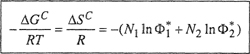
It is convenient to write the thermodynamic mixing properties as the sum of two parts: (1) a combinatorial, contribution that appears in the entropy (and therefore in the Gibbs energy and in the Helmholtz energy) but not in the enthalpy or in the volume of mixing; and (2) a residual contribution, ⁵ determined by differences in intermolecular forces and in free volumes⁶ between the components. For the entropy of mixing, for example, we write⁷

⁵ The residual contribution to a mixing property is defined as the observed change in that property upon mixing (at constant T and P) minus the calculated change in that property upon mixing (at the same T, P, and composition), where the calculation is based on a model that serves as a reference. Two common reference models are the ideal solution and the athermal solution. Residual mixing properties are different from residual properties discussed in App. B.

⁶ In general, two pure liquids have different free volumes due to different coefficients of thermal expansion. According to the Prigogine-Flory-Patterson theory, discussed in Sec. 8.2, two liquids with different free volumes experience a net contraction upon mixing and, therefore, negative contributions appear in both Δ_mixH and Δ_mixS. Contributions from free-volume differences and from differences in contact energy are included in the residual part of a mixing property.

⁷ In most, but not all cases, ΔS^C is the dominant term.

(8–3)

where superscript C stands for combinatorial and superscript R stands for residual.

Consider a mixing process where the molecules of fluids 1 and 2 have no difference in molecular interactions and no difference in free volume. For this case, isothermal, isobaric mixing occurs also at constant volume; the residual mixing properties are zero and we are concerned only with combinatorial mixing properties.

Using the concept of a quasicrystalline lattice as a model for a liquid, an expression for the combinatorial entropy of mixing was derived independently by Flory (1941, 1942) and by Huggins (1942) for flexible chain molecules that differ significantly in size. The derivation, based on statistical arguments and several well-defined assumptions, is not reproduced here. It is presented in several references (Fast, 1962; Flory, 1953); we give here only a brief discussion along with the result.

We consider a mixture of two liquids 1 and 2. Molecules of type 1 (solvent) are single spheres. Molecules of type 2 (polymer) are assumed to behave like flexible chains, i.e., as if they consist of a large number of mobile segments, each having the same size as that of a solvent molecule. Further, it is assumed that each site of the quasilattice is occupied by either a solvent molecule or a polymer segment and that adjacent segments occupy adjacent sites. Let there be N₁ molecules of solvent and N₂ molecules of polymer and let there be r segments in a polymer molecule. The total number of lattice sites is (N₁ + rN₂). Fractions and of sites occupied by the solvent and by the polymer are given by

(8–4)

Flory and Huggins have shown that if the amorphous (i.e., noncrystalline) polymer and the solvent mix without any energetic effects (i.e., athermal behavior), the change in Gibbs energy and entropy of mixing are given by the remarkably simple expression:

(8–5)

The entropy change in Eq. (8-5) is similar in form to that of Eq. (7-80) for a regular solution except that segment fractions are used rather than mole fractions. For the special case r = 1, the change in entropy given by Eq. (8-5) reduces to that of Eq. (7-80), as expected. However, when r > 1, Eq. (8-5) always gives a combinatorial entropy larger than that given by Eq. (7-80) for the same N₁ and N₂. Much discussion of these equations has led Hildebrand (1947) to the conclusion that for nonpolar systems, Eq. (7-80) gives a lower limit to the combinatorial entropy of mixing and Eq. (8-5) gives an upper limit; the “true” combinatorial entropy probably lies in between, depending on the size and shape of the molecules.

Modifications of Eq. (8-5) have been presented by several authors, including Huggins (1941, 1942), Guggenheim (1944, 1952), Staverman (1950), Tompa (1952), and Lichtenthaler (1973, 1974).⁸

⁸ Various models are compared in a review by S. G. Sayegh and J. H. Vera, 1980, Chem. Eng. J., 19: 1.

The modifications introduced by Lichtenthaler, similar to those of Tompa, provide a reasonable method for calculating ΔS^C for mixtures of molecules differing in shape as well as size. The model of Lichtenthaler assumes that the ratio of the molecular (van der Waals) volumes of the polymer and the solvent (regarded as monomer) gives r, the number of segments of the polymer molecule. Similarly, the ratio of the surface areas of the polymer and the solvent gives q, the external surface area of a polymer molecule. The ratio q/r is a measure of the shape of the polymer molecule; for a monomer q/r = 1. As r becomes very large, for a linear chain q/r → 2/3 and for a sphere (or cube) q/r → 0. For globular molecules, the ratio q/r lies between zero and unity.

Combinatorial entropies of mixing calculated with Lichtenthaler’s expression lie between those found from Eqs. (7-80) and (8-5), depending on ratio q/r If molecules 1 and 2 are identical in size and shape, q = r = 1 and the expression of Lichtenthaler reduces to Eq. (7-80). If the coordination number⁹ becomes very large, q/r → 1 and the expression of Lichtenthaler becomes identical to Eq. (8-5), regardless of molecular shape.

⁹ Coordination number is the number of nearest neighbors around a solvent molecule or segment. See Sec. 7.4.

To illustrate, Fig. 8-2 shows excess combinatorial entropies per mole of sites¹⁰ for mixtures of benzene and various forms of polyethylene. This figure shows that the combinatorial entropy is strongly affected by the bulkiness of the large molecule that increases with decreasing qlr. The Flory-Huggins expression [Eq. (8-5)] does not distinguish between the six cases shown in Fig. 8-2.

¹⁰ The excess combinatorial entropy is defined, as usual, as the entropy of mixing in excess of that for an ideal system. While entropies usually are calculated per mole of mixture, we can convert to entropies per mole of sites by writing

where is given by Eq. (8-4).

Figure 8-2 Excess combinatorial entropy per mole of sites for benzene/polyethylene. Curves A to F refer to different shapes assumed for polyethylene (r = 1695):
A = straight-chain, (q/r) = 0.788;
B = double-strand flat ribbon, (q/r) = 0.591;
C = quadruple-strand flat ribbon, (q/r) = 0.493;
D = rod-like shape, (q/r) = 0.394;
E = rod-like shape, but shorter axis and larger cross-section as in D, (q/r) = 0.127;
F = cube, (q/r) = 0.076.

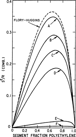
Since the Flory-Huggins formula depends only on the size ratio r, the same in all six cases, it always gives the same result (dashed curve in Fig. 8-2), independent of molecular shape. Since Flory-Huggins assumes that q/r = 1, it gives an upper limit for the combinatorial entropy of mixing; therefore, the results are close to those shown by curve A with the highest value of q/r. For mixtures of bulky molecules, even if they differ significantly in size, q/r is much smaller than 1 (case F) and then the ideal entropy of mixing [Eq. (7-80)] is a much better approximation than Eq. (8-5).

Donohue (1975) has presented a discussion of Lichtenthaler’s model for the combinatorial entropy of mixing and has shown how it can be quantitatively transformed into a generalized Flory-Huggins expression.

Although the simple expression of Flory and Huggins does not always give the (presumably) correct, quantitative combinatorial entropy of mixing, it qualitatively describes many features of athermal polymer solutions. Therefore, for simplicity, we use it in our further discussion of polymer solutions in this section.

The expression of Flory and Huggins immediately leads to an equation for the excess entropy that is, per mole of mixture,

(8–6)

By algebraic rearrangement of Eq. (8-6) and expansion of the resulting logarithmic terms, it can be shown that for all r > 1, s^E is positive. Therefore, for an athermal solution of components whose molecules differ in size, the Flory-Huggins theory predicts negative deviations from Raoult’s law:

(8–7)

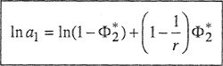
For an athermal solution, the activity of the solvent from Eq. (8-6) is

(8–8)

and the corresponding activity coefficient (based on mole fraction) is¹¹

¹¹ In the limit → 1, the activity coefficient for a solvent in a polymer solution based on mole fraction is awkward, as in this limit γ₁ → –∞ for large values of r. For polymer solutions, the activity coefficient of the solvent is more conveniently defined on a weight-fraction or volume-fraction basis, as pointed out by D. Patterson, Y. B. Tewari, H. P. Schreiber, and J. E. Guillet, 1971, Macromolecules, 4: 356.

(8–9)

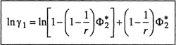
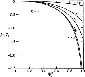
Figure 8-3 shows activity coefficients for the solvent according to Eq. (8-9) for several values of parameter r that provides a measure of the disparity in molecular size between the two components. The activity coefficient is a strong function of r for small values of that parameter, but for large values (r ≥ 100) the activity coefficient is essentially independent of r. For solutions of polymers in common solvents, r is a very large number and we can see in Fig. 8-3 that large deviations from ideal-solution behavior result merely as a consequence of differences in molecular sizes even in the absence of any energetic (enthalpy of mixing) effects.

Figure 8-3 Solvent activity coefficient in an athermal polymer solution according to the equation of Flory and Huggins. Parameter r gives the number of segments in the polymer molecule.

To apply the theoretical result of Flory and Huggins to real polymer solutions, i.e., to solutions that are not athermal, it has become common practice to add to the combinatorial part of the Gibbs energy, given by Eq. (8-5), a semiempirical part for the residual contribution. In other words, we add a term that, if there is no difference in free volumes, is given by the enthalpy of mixing. The form of this term is the same as that used in the van Laar-Scatchard-Hildebrand theory of solutions (see Secs. 7.1 and 7.2); the excess enthalpy is set proportional to the volume of the solution and to the product of the volume fractions. The Flory-Huggins equation for real polymer solutions then becomes

(8–10)

The activity of the solvent is given by

(8–11)

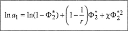
and the corresponding equation for the activity coefficient of the solvent (based on mole fraction) is

(8–12)

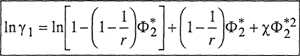
where χ, the Flory-Huggins interaction parameter, is determined by intermolecular forces. Figure 8-4 shows activity coefficients for the solvent according to the Flory-Huggins equation for real polymer solutions.

Figure 8-4 Solvent activity coefficient in a real polymer solution according to the equation of Flory and Huggins. Parameter χ depends on the intermolecular forces between polymer and solvent.

Dimensionless parameter χ is assumed to be independent of composition.¹² It is determined by the energies that characterize the interactions between pairs of polymer segments, between pairs of solvent molecules, and between one polymer segment and one solvent molecule. In terms of the interchange energy [Eq. (7-71)], χ is given by

¹² However, as found from experiment, and as predicted from more sophisticated theories (compare Sec. 8.3), χ varies with polymer concentration, sometimes appreciably, contrary to the simple Flory-Huggins theory discussed here. The advanced theories are based on an equation of state that, unlike lattice theory, permits components to mix (at constant pressure and temperature) with a change of volume.

(8–13)

Assuming that the interchange energy w is independent of temperature, Flory parameter χ is inversely proportional to temperature. In this case, the interchange energy refers not to the exchange of solvent and solute molecules but rather to the exchange of solvent molecules and polymer segments. For athermal solutions, χ is zero, and for mixtures of components that are chemically similar, χ is small compared to unity.

Equations (8-10) to (8-12) have been used widely to describe thermodynamic properties of solutions whose molecules differ greatly in size. For example, Fig. 8-5 shows activity coefficients at infinite dilution for n-butane and n-octane in n-alkane solvents (n-C₂₀H₄₂ to n-C₃₆H₇₄),¹³ measured by gas-liquid chromatography.¹⁴ Figure 8-5 shows that negative deviations from Raoult’s law rise with increasing difference in molecular size between solute and solvent. As the components are chemically similar, χ is expected to be small, and therefore deviations from ideal-solution behavior result mainly from differences in molecular size. A similar result is indicated in Fig. 8-6 that shows activity coefficients for n-heptane in the n-heptane/polyethylene system.

¹³ Data from J. F. Parcher et al, 1975, J. Chem. Eng. Data, 20: 145.

¹⁴ This experimental method is discussed briefly in App. F.

Figure 8-5 Activity coefficients at infinite dilution for n-butane and n-octane in n-alkane solvents near 100°C. Negative deviations from Raoult’s Saw are due to the difference in molecular size.

Figure 8-6 Activity coefficients of heptane in the n-heptane (1)/polyethylene (2) system at 109°C.

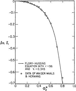
Figure 8-7 shows how Eq. (8-11) may be used to reduce data on rubber solutions to obtain Flory-Huggins parameter χ. In Fig. 8-7, 1/r has been set equal to zero. For these systems, Eqs. (8-11) and (8-12) give an excellent representation of the data but for many other systems representation is poor because, contrary to the simple theory, χ varies with polymer concentration.

Figure 8-7 Data reduction using the equation of Flory and Huggins. Data are for solutions of rubber near room temperature, interaction parameters χ are given by the slopes of the lines.

If we set r equal to the ratio of molar volumes of polymer and solvent, then the segment fraction Φ* given in Eq. (8-4) is identical to the volume fraction in the Scatchard-Hildebrand theory, Eqs. (7-25) and (7-26). In terms of solubility parameters, it can then be shown that χ is given by

(8–14)

where υ₁ is the molar volume of the solvent and δ₁ and δ₂ are, respectively, the solubility parameters of solvent and polymer. Equation (8-14) is not useful for an accurate quantitative description of polymer solutions but it provides a good guide for a qualitative consideration of polymer solubility. For good solubility, χ should be small or negative, as discussed below. According to the Scatchard-Hildebrand theory for nonpolar components, χ cannot be negative; however, in many polar systems negative values have been observed.

A criterion of a good solvent for a given polymer is

(8–15)

Equation (8-15) provides a useful practical guide for nonpolar systems (Burrel, 1955; Blanks and Prausnitz, 1964) and for polar systems an approximate generalization of Eq. (8-14) has been suggested by Blanks (1964), Hansen (1967, 1967a, 1971), and Barton (1990).

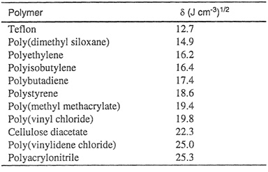
Table 8-1 gives solubility parameters for some noncrystalline polymers. When these are compared with solubility parameters for common liquids (see Table 7-1), some qualitative statements concerning polymer solubility can easily be made. For example, the solubility parameters show at once that polyisobutylene (δ = 16.4) should be readily soluble in cyclohexane (δ = 16.8) but only sparingly soluble in carbon disulfide (δ = 20.5).

Table 8-1 Solubility parameters for some amorphous polymers near 25°C (Gruike, 1989).

It is important to keep in mind that all of the relations given in this section are restricted to amorphous polymers; they are not directly applicable to crystalline, glassy or cross-linked polymers.

Although the Flory-Huggins equation for real polymer solutions does not provide an accurate description of the thermodynamics properties of such solutions, this relatively simple theory contains most of the essential features that distinguish solutions of very large molecules from those containing only molecules of ordinary size.

The addition of a residual term to the theoretical result for athermal mixtures is essentially an empirical modification to obtain a reasonable expression for the Gibbs energy of mixing. According to the theory, χ should be independent of polymer concentration and of polymer molecular weight, but in many, especially polar systems, χ changes considerably with both (Koningsveld et al., 1968, 1970. 1971; Siow et al., 1972; Orwoll, 1977). Further, the theory erroneously assumes that the enthalpy of mixing should be given by the last term in Eq. (8-10); however, calorimetric enthalpy-of-mixing data often give a value of χ significantly different from that obtained when experimental activities are reduced by Eq. (8-11). This follows, in part, because values of χ obtained from Eqs. (8-10) to (8-12) are directly associated with the Flory-Huggins approximation for the combinatorial contribution; a different approximation for the combinatorial contribution necessarily produces a change in χ. Therefore, the value of χ obtained from experimental activities has an entropic as well as enthalpic part. Finally, experimental results by many researchers show clearly that the temperature dependence of χ is not a simple proportionality to inverse temperature.

When applied to liquid-liquid equilibria, the simple Flory-Huggins theory can only explain partial miscibility of polymer/solvent systems at low temperatures. The combinatorial entropy always favors mixing and therefore, if χ is zero or negative, complete miscibility is obtained at any temperature. If χ > 0, however, there exists an upper limit where partial miscibility occurs. When Eq. (8-10) for the Gibbs energy of mixing is combined with the equations for stability (see Sec. 6.12), the condition for complete miscibility of components 1 and 2 is given by

(8–16)

The equal sign characterizes incipient instability where χ is designated by its critical value χ^c and that occurs at the critical composition

(8–17)

In polymer solutions, when r >> 1, the critical value χ^c is essentially 1/2. The critical composition occurs at a very small polymer concentration, approaching zero as r → ∞. For ordinary solutions, when r = 1, the critical values axe χ^c = 2 and in agreement with results discussed in Sec. 7.6. The critical temperature T^c for phase separation is an upper critical solution temperature (UCST); i.e. for T > T^c there is only one liquid stable phase (complete miscibility), whereas for T < T^c there are two stable liquid phases. In a polymer/solvent system, the limiting UCST for a polymer of infinite molecular weight is known as the (theta) θ temperature. Because χ is inversely proportional to temperature [Eq. (8-13)], it can be expressed as

(8–18)¹⁵

¹⁵ Comparison of Eqs, (8-16) and (8-18) shows that χ^c(T= θ) = 1/2.

If θ is known for a polymer/solvent system, Eq. (8-18) can be used to calculate χ(T) if the molecular weight is very high.

Figure 8-8 shows calculated phase diagrams for binary mixtures according to the simple Flory-Huggins theory. From r = 1 to r → ∞, the reduced UCST increases by a factor of 4.

Figure 8-8 Calculated phase diagrams (cloud-point curves) for a binary mixture according to the Flory-Huggins theory. The dotted line shows the locus of upper critical solution temperatures.

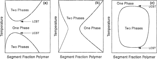
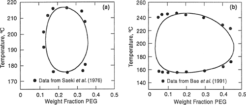
Although not predicted by the simple theory, partial miscibility at higher temperatures (LCST) has been observed for many polymer/solvent systems (Siow et al, 1972), as indicated in Fig. 8-9(a). With increasing molecular weight, the difference between LCST and UCST tends to decrease, resulting ultimately in an “hourglass” type of phase diagram, when the two regions of limited miscibility have merged. In that case, complete miscibility is not obtained in the entire temperature range, as shown in Fig. 8-9(b). However, as discussed in Sec. 6.13, the LCST may occur at temperatures below the UCST, resulting in a closed-loop phase behavior shown in Fig. 8-9(c). A realistic qualitative explanation of this phenomenon was given many years ago by Hirschfelder et al. (1937). Closed-loop behavior follows from competition among three contributions to the Helmholtz energy of mixing: dispersion forces, combinatorial entropy of mixing, and highly oriented specific interactions (such as hydrogen bonding). While the dispersion forces energetically favor phase separation, the combinatorial entropy of mixing favors mutual miscibility. The specific interactions are energetically favorable, but entropically unfavorable, because of their highly directional-specific character. Therefore, in the presence of specific interactions between dissimilar components, the mixture could form a single homogeneous phase at low temperatures where the energy of specific interactions compares favorably to thermal energy kT. At moderate temperatures, where neither specific interactions nor combinatorial entropy of mixing dominate, the effect of dispersion forces becomes significant and the mixture exhibits phase separation. At higher temperatures, the combinatorial entropy of mixing becomes dominant and a single homogeneous phase reappears.

Figure 8-9 Schematic representation of phase stability in three binary polymer solutions, (a) UCST is below LCST; (b) hourglass; (c) dosed loop, where LCST is below UCST.

Using essentially empirical arguments, Qian and coworkers (1991; 1991a) introduced into the original Flory-Huggins lattice theory a χ, parameter given by the product of two functions, one depending on composition and the other on temperature. This semiempirical model permits fitting most observed types of binary liquid-liquid phase diagrams (UCST, LCST, UCST and LCST, hourglass, and closed loop) by adjusting the coefficients in the functions that give the desired temperature dependence and composition dependence of χ. Extensions and simplifications in Qian’s work were reported by Bae and coworkers (1993).

Bae et al. (1993) assigned empirical composition and temperature dependencies to Flory parameter χ:

(8–19)

with

(8–20)

and

(8–21)

where d₀, d₁, d₂, and b are binary parameters.

Using the adjustable binary parameters given in Table 8-2, Bae et al. obtained good fits of LLE data, as Figs. 8-10 and 8-11 show. Figure 8-10 compares calculated and experimental cloud-point curves for the poly(ethylene glycol) (PEG)/water system. Molecular weights of PEG are 3,350, 8,000, and 15,000 g mol^–1. Solid lines in the closed-loop phase diagram are calculated; they fit experimental data well.

Figure 8-10 Phase diagrams for three PEG/water systems showing cloud-point temperatures as functions of PEG weight fractions. The molecular weight of PEG is 3,350 g mol^-1 (); 8,000 g mol^-1 (), and 15,000 g mol^-1 (o). Solid lines are calculated (Bae et al., 1993).

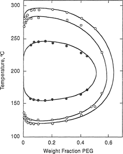
Figure 8-11 Phase diagrams for two PS/PVME systems showing cloud-point temperatures as functions of polystyrene weight fractions. The molecular weights of PS are 50,000 g mol^-1 (), and 100,000 g mol^-1 (o). Solid lines are calculated (Bae et al., 1993).

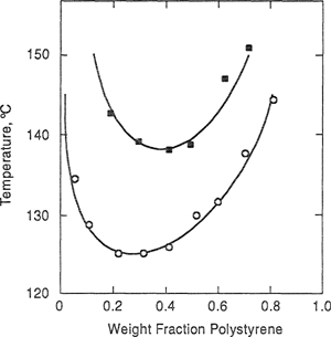
Table 8-2 Binary parameters* of the empirically extended Flory-Huggins model [Eqs. (8-22) and (8-24)]. PEG= Poly(ethylene glycol); PS = Poly(styrene); PVME = Poly(vinyl methyl ether). The weight-average molecular weight of PVME is = 99,000 g mol^-1.

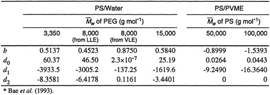
Figure 8-11 shows the cloud-point curves of two polymer blend systems: poly(styrene) (PS)/poly(vinyl methyl ether) (PVME) for two different molecular weights of PS. This system exhibits LCST that declines with increasing molecular weight of PS. The polydispersity index of PVME (/ ≈ 2.1) shows that PVME is not a monodisperse polymer, and therefore the equations for a binary system are not truly applicable. Nevertheless, the solid lines calculated using the adjustable parameters in Table 8-2 agree well with experiment.

The empirically extended Flory-Huggins model has essentially no theoretical basis beyond that of the original Flory-Huggins equation. The extended model has a simple algebraic form, uses a few adjustable parameters, and appears to be suitable for representing vapor-liquid and liquid-liquid equilibria, including closed-loop phase diagrams. However, it has no predictive value. Given binary experimental data, the extended Flory-Huggins model is useful only for representing the data in an oversimplified molecular-thermodynamic framework.

A variety of polymer-solution theories has been developed since the original work of Flory and Huggins in the early 1940’s. Some proposed theories are extensions of the Flory-Huggins equation, based on a close-packed lattice.

For example, Freed and coworkers (Freed, 1985; Bawendi et al, 1987, 1988; Madden et al., 1990, 1990a) developed a lattice-field theory for polymer solutions that, in principle, provides an exact mathematical solution of the Flory-Huggins lattice, that is, Freed et al. avoid the simplifying assumptions made by Flory and Huggins. In Freed’s theory, good agreement was found between calculated values and the computer simulation data of Dickman and Hall (1986). It has also been applied successfully to polymer blends (Dudowicz and Freed, 1991).

Based on Freed’s lattice-field theory, Hu and coworkers (1991) reported a double-lattice model for the Helmholtz energy of mixing for binary polymer solutions. This model includes specific interactions such as hydrogen bonding.

A simple molecular-thermodynamic model was developed by Hino et al. (1993). Using the incompressible lattice-gas model of ten Brincke and Karasz (1984), Hino et al. introduced specific interactions into the expression of the Helmholtz energy of mixing obtained by Lambert et al. (1993) by correlating Monte-Carlo-simulation results. Hino’s model is conceptionally and mathematically simple. Hino considered a binary mixture of components 1 and 2 that may form specific interactions between similar components and between dissimilar components. Each contact point of a molecule is assumed to interact either in a specific manner with interaction energy ε_ij + δεij or in a nonspecific manner with interaction energy ε_ij, where i = 1 and j = 1 or 2. Both ε_ij and δε_ij are negative and independent of temperature. Hino assumed that a fraction, f_ij, of the i-j interactions is specific and a fraction 1-f_ij is nonspecific. To obtain a simple expression for the internal energy of mixing, Δ_mixU, Hino also assumed that f_ii in the mixture is identical to that in pure i. A similar assumption is made for f_jj. These assumptions are consistent with the assumption that f_ij depends only on temperature, but is independent of composition, as indicated by Eq. (8-26). With these assumptions, Δ_mixU is given by

(8–22)

where N₁₂ is the total number of 1-2 pairwise contacts and ω is defined by:

(8–23)

where ε is an interchange energy:

(8–24)¹⁶

¹⁶ The interchange energy defined here is similar, but not identical, to that given in Eq. (7-71).

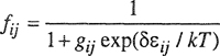
Further, Hino assumed that f_ij is given by the Boltzmann distribution law:

(8–25)

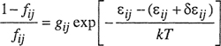
where g_ij is the ratio of the degeneracy of nonspecific i-j interactions; f_ij is therefore given by:

(8–26)

The Helmholtz energy of mixing (Δ_mixA) is obtained by integrating the Gibbs-Helmholtz equation using Guggenheim’s athermal entropy of mixing as the boundary condition:

(8–27)

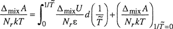
with

(8–28)

where N_r is the total number of lattice sites and is a dimensionless temperature defined as

(8–29)

Here, r_i, and θ_i are, respectively, the number of segments per molecule, volume fraction, and surface fraction of component i. and θ_i are defined by

(8–30)

(8–31)

where N_i and q_i are, respectively, the number of molecules and the surface area parameter of component i; q_i is related to the number of surface contacts per molecule, zq_i, defined as

(8–32)

where z is the lattice coordination number. Hino uses a simple cubic lattice (z = 6).

The expression used for N₁₂ is based on the expression obtained by Lambert et al. (1993) by correlating Monte-Carlo-simulation results for several monomer/r-mer mixtures:

(8–33)

where

(8–34)

(8–35)

(8–36)

(8–37)

(8–38)

The numerical coefficients in Eqs. (8-35) to (8-38) follow from Monte-Carlo calculations. The temperature dependence of N₁₂ is expressed in terms of the dimensionless temperature, now given as kT/ω.

In this model, the number of segments for the smaller molecule, r₁ is always set equal to 1. For mixtures containing low-molecular-weight species, r₂ is determined either from the ratio of UNIQUAC size parameters, proportional to the van der Waals molecular volumes, or r₂ is set equal to the ratio of molar volumes at room temperature. Therefore, size parameter r₂ is not an adjustable parameter, but a preset physical parameter. The adjustable parameters for a binary mixture are energy parameter ε for nonspecific interactions and degeneracy parameter g_ij and energy parameter δε_ij for specific interactions, where i = 1 or 2 and j = 1 or 2. All these adjustable parameters are determined from experimental data.

For a number of polymer/solvent mixtures, the model of Hino et al. (1993) can describe closed-loop phase behavior considering specific interactions between dissimilar components only. Making reasonable assumptions, Hino assigned g₁₂ = 5000 and calculated ε from at UCST or LCST and δε₁₂ from the experimental ratio of UCST to LCST. As an example, Fig. 8-12 compares theoretical coexistence curves with experimental data for the system poly(ethylene glycol)/water with two molecular weights of the polymer. Although specific interactions were introduced in a simple way, Hino’s model compares favorably with the experimental data.

Figure 8-12 Temperature-composition coexistence curves for the system poly(ethylene giycol)/water. (a) _η = 2,190 g mol^-1; (b) _η = 3,350 g mol^-1;—— model of Hino et al. (1993).

To account for compressibility and density changes upon isothermal mixing, Sanchez and Lacombe (1976, 1977, 1978), Costas and Sanctuary (1981, 1984), Panayiotou and Vera (1982), and Kleintjens and Koningsveld (1980, 1982) developed new forms of a lattice-fluid model based on FIory-Huggins theory; the central idea here is to use a lattice where some lattice points are not occupied (holes). Sanchez and Balazs (1989) introduced corrections for oriented interactions between dissimilar components. Panayiotou and Sanchez (1991) modified the lattice-fluid theory for polymer solutions to account for strong interactions (hydrogen bonding) between polymer and solvent. Their model is in the form of an equation of state suitable for describing thermodynamic properties of polymer solutions over an extended range of external conditions from the ordinary liquid state to high temperatures and pressures where the solvent may be supercritical, as briefly discussed in the next section.

8.3 Equations of State for Polymer Solutions

Lattice models, discussed in Sec. 8.2, often can describe the main characteristics of liquid mixtures containing nonpolar molecules differing in size and shape. In regular-solution theory, a particular combinatorial entropy of mixing is joined with a simple expression for the energy of mixing obtained from summing the energies of interaction between neighboring sites. However, for quantitative work, this simple approach is inadequate when tested against experimental data. Even for mixtures of n-alkanes (Flory et al., 1964, 1965, 1967), the excess thermodynamic properties cannot be described satisfactorily by lattice theory. In particular, changes of volume upon mixing are beyond the scope of such theory. However, experiments show that when liquid mixtures are formed at constant temperature and pressure, small changes of volume upon mixing are the rule rather than the exception, even for mixtures of nonpolar molecules.

Observed excess entropies of mixtures often deviate markedly from calculated combinatorial contributions. That deviation, coupled with observed changes of volume upon mixing, directs attention to the major deficiency of lattice theory: the need to take into account additional properties of the pure components beyond those that reflect molecular size and potential energy. These properties are manifested in P-V-T behavior, or in the equation of state.

In general, pure fluids have different free volumes, i.e. different degrees of expansion. When liquids with different free volumes are mixed, that difference contributes to the excess function. Differences in free volumes must be taken into account, especially for mixtures of liquids whose molecules differ greatly in size. For example, in a solution of a polymer in a chemically similar solvent of low molecular weight, there is little dissimilarity in intermolecular interactions but the free volume dissimilarity is significant. The low-molecular-weight solvent may be much more dilated than the liquid polymer; the difference in dilation (or free volume) has an important effect on solution properties. An example is propane and polyethylene at room temperature, where propane, far above its normal boiling point, is much dilated while polyethylene is not.

To develop an equation of state (EOS) for liquids and liquid mixtures, one convenient way is to start with an expression for the canonical partition function utilizing concepts similar to those used by van der Waals. The Prigogine-Flory-Patterson theory (Prigogine, 1957; Flory, 1965, 1970; Patterson, 1969, 1970) provides a successful example. Another possibility is to construct a partition function for large molecules to provide an equation of state based on a lattice-with-holes theory, as discussed, for example by Bonner et al. (1972) and developed by Eichinger and Flory (1968) and Simha and Somcynsky (1969, 1971); a successful version, developed by Sanchez and Lacombe (1976, 1977), has been extended by Panayiotou and Sanchez (1991) to include associated polymer solutions.

Advances in statistical thermodynamics have brought to the forefront tangent-sphere models of chain-like fluids. These models abandon the lattice picture; they mode! polymers as freely-jointed tangent-spheres where nonbonded spheres interact through a specified intermolecular potential. These are, for example, the generalized Flory model developed by Hall and coworkers (Dickman and Hall, 1986; Honnell and Hall, 1989; Smith et al, 1995), and, as introduced in Sec. 7.17, the statistical-associated-fluid theory (SAFT) developed by Chapman et al. (1990) and the perturbed-hard-sphere-chain (PHSC) theory of Song et al. (1994).

Lambert et al. (1998) give a comprehensive review of equations of state for molten polymers and for mixtures of polymers with solvents or other polymers. We present here a brief survey of some equations of state and the basic ideas for their derivation.

Prigogine-Flory-Patterson Theory

This statistical-thermodynamic model is based on the fundamental ideas of van der Waals:

• The structure of a fluid is determined primarily by the molecules’ repulsive forces.

• The contribution of attractive forces is taken into account by assuming that the molecules are situated in a homogeneous and isotropic field determined by the (attractive) intermolecular potential. This field follows from averaging (smearing) attractive forces. A consequence of this averaging is that, at constant composition, the field is given by simple functions of density and temperature.

Numerous articles have presented van der Waals-type theories for dense fluids containing small, spherical molecules (Henderson, 1974; Swinton, 1976). However, only a few authors (Flory, 1970; Patterson, 1969, 1970) have applied these ideas to fluids containing large molecules, because for such molecules consideration must be given to external¹⁷ (rotational, vibrational) degrees of freedom in addition to translational degrees of freedom. An approximation for doing so was suggested by Prigogine (1957) but since this approximation is valid only at high (liquid-like) densities, care must be taken when using Prigogine’s suggestion over a wide density range. As pointed out by Scott and van Konynenburg (1970), theories using Prigogine’s assumption are qualitatively incorrect at low densities, unless that assumption is modified, as indicated in Sec. 7.15.

¹⁷ Here external refers to those (high-amplitude, low-frequency) rotations and vibrations that depend on density. The division between external and internal is somewhat arbitrary. At very high densities, all degrees of freedom are external.

For liquid mixtures, especially polymer solutions, the Prigogine-Flory-Patterson theory has proved to be useful. We now summarize the essential steps in that theory. First, we discuss pure liquids and then extend the discussion to liquid mixtures.

As shown in Sec. 7.15, the generalized van der Waals partition function for a one-component polyatomic fluid can be written as

(8-39)

where N is the number of molecules in total volume V at temperature T, E₀/2 is the mean intermolecular potential energy experienced by one molecule due to the attractive forces from all other molecules, and Λ is the de Broglie wavelength that depends only on temperature and molecular mass. V_f is the free volume, i.e., the volume available to the center of mass of one molecule as it moves in volume V. The product [q_ext(V)q_int(T)] =q_r,v [see Eq. (7-219)] represents the contribution (per molecule) from rotational and vibrational degrees of freedom, whereas contributions from translational degrees of freedom are given by the first bracketed term of Eq. (8-39).¹⁸

¹⁸ The meaning of q used here should not be confused with that used in earlier sections of this chapter.

Following Flory (1964, 1965, 1967, 1970) we subdivide each of the N molecules into r segments. The definition of a segment is essentially arbitrary; e.g., it is appropriately considered to be an isometric portion of a chain molecule.¹⁹

¹⁹ For r > 1, a combinatorial factor Q^c has to be included in Eq. (8-39) to take into account the degeneracy caused by disposition of segments in space. In terms of a lattice model (compare Sec. 8.2), Q^c expresses the number of ways of arranging the segments of N molecules over a spatial array of rN sites. As long as we are concerned only with the equation of state, specification of Q^c is not required; it suffices here to assume that it is independent of volume. In that event, it does not contribute to the equation of state.

For large, polyatomic molecules in a condensed phase, the number of external degrees of freedom cannot be estimated from first principles. Instead, we define a parameter c (per segment) such that 3rc is the number of effective external degrees of freedom per molecule.²⁰ In this context, “effective” follows from Prigogine’s approximation that external rotational and vibrational degrees of freedom can be considered as equivalent translational degrees of freedom. This assumption enables us to postulate a useful expression for [(V_fΛ^-3)q_ext]:

²⁰ Here parameter c is defined per segment. In Chaps. 7 and 12, c is defined per molecule.

(8-40)

For argon-like molecules (r = 1), rc = 1, and for all other molecules (r > 1), rc > 1. Product rc reflects the number of rotational and vibrational motions per molecule that are affected by the presence of neighbors. Indirectly, therefore, rc is often a measure of molecular size because a large molecule has more external rotations and vibrations than a small molecule. However, product rc reflects also the looseness (or flexibility) of a molecule. Thus rc for a stiff rod is smaller than that for a soft (rubberlike) rod having the same number of segments.

To reduce the partition function to practice after substituting Eq. (8-40) into Eq. (8-39), we require expressions for the free volume V_f-and potential energy E₀.

For the free volume V_f for one molecule containing r segments Flory (1970) assumes

(8-41)

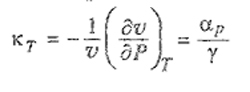
where υ* is the characteristic or hard-core volume of a segment, =υ/υ* is the reduced volume, υ = V/(Nr) (i.e., the volume available to one segment), and τ is a numerical factor.²¹

²¹ Specification of τ is not required because it disappears in the process of differentiation, for obtaining the equation of state and it cancels in taking differences with respect to the pure components when deriving excess functions for mixtures.

In view of the short range of attractive forces operating between uncharged molecules, potential energy E_º may be considered additive in the molecular surface areas of contact. Therefore Flory proposed for one molecule,

(8-42)

where s is the number of contact sites per segment²² (proportional to the surface area per segment) and -nη/υ is the intermolecular energy per contact.

²² s ≈ q/r where q is the number of contact sites per molecule. For a simple long chain, q is related to r by zq = r(z - 2) = 2, where z is the lattice coordination number; however, for model flexibility, Flory preferred to avoid using an explicit lattice geometry. Therefore, the relation between, s and r remained unspecified.

Substitution of Eqs. (8-40) to (8-42) into Eq. (8-39) gives a partition function of the form

(8-43)

where the reduced temperature is defined by

(8-44)

and the “constant” is independent of V²³ From Eq. (8-43), the equation of state is obtained by differentiation according to Eq.(7-209). Expressed in reduced form, it is²⁴

²³ While “constant” depends on N and T, this is of no concern in deriving the equation of state.

²⁴ Because of Eq.(8-40), Eq.(8-45)is restricted to liquids whenever rc > 1.

(8–45)

where the reduced pressure is

(8–46)

The characteristic parameters P*, v*, and T* satisfy the equation

(8–47)

To use the equation of state, we must know the characteristic parameters. For pure fluids, these parameters can be determined from volumetric data in several ways. One method, proposed by Flory (1964, 1965, 1967) is to determine them from data at (essentially) zero pressure for density, thermal expansion coefficient α_p, and thermal pressure coefficient γ. In the limit P → 0 the equation of state takes the simple form

(8–48)

For liquids at (essentially) zero pressure, it follows that

(8–49)

where

(8–50)

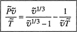
If experimental data are available for v as a function of T, these equations suffice to determine and ; then, for a given υ and T, we obtain v* and T*. Differentiation of Eq.(8-45) with respect to temperature, followed by substitutions into Eqs. (8-46) and (8-47), yields

(8–51)

where γ ≡ (∂PI∂T)_v taken in the limit at zero pressure.²⁵

²⁵ Coefficients α_p and γ are related to isothermal compressibility k_r through

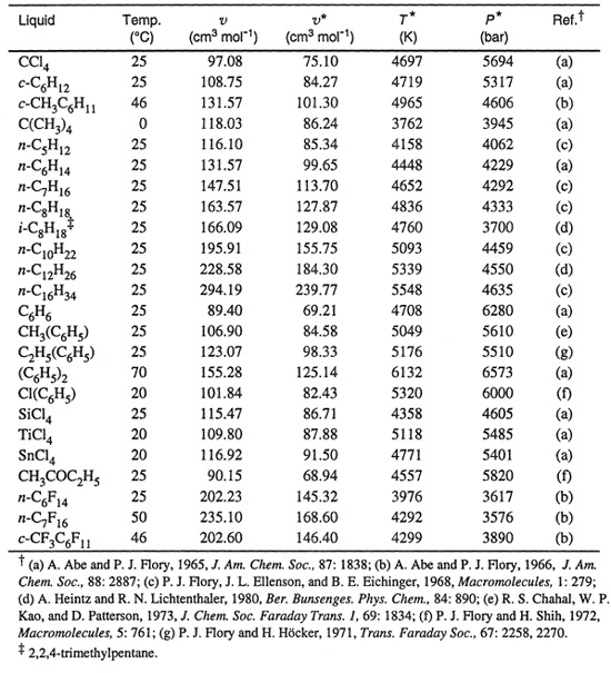
The advantage of Flory’s method is that volumetric data for liquids are required only at low (e.g., atmospheric) pressure. However, very accurate experimental values of α and γ are necessary and these are often not available. Further, when determined by this method, the parameters are temperature dependent. Table 8-3 gives characteristic parameters of common solvents and Table 8-4 gives parameters for some common polymers at various temperatures.

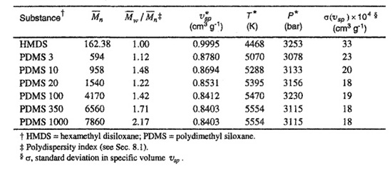
Another method to determine the characteristic parameters is to fit P-V-T data directly to Eq.(8-45) over a wide range of pressures and temperatures. Lichtenthaler et al. (1978) used this method to determine characteristic parameters for seven dimethyl-siloxane polymers of different molecular weights. Their results are given in Table 8-5, where the last column shows that the Prigogine-Flory equation of state represents all P-V-T data with a standard deviation of better than ±0.3%. (Better agreement could be obtained by letting parameters v*, T*, and P* vary slightly with temperature).

To extend Eq.(8-43) to mixtures, we use two assumptions:

1. Hard-core volumes of the components are additive.

2. The intermolecular energy depends in a simple way on the surface areas of contact between solvent molecules and/or segments.

The first assumption is implicit in the partition function. The second assumption was anticipated by Eq.(8-42), expressing the energy as proportional to the surface as measured by the number of contact sites (per segment) s. Equation (8-42) rests on the assumption that intersegnienta! attractions are short range when compared with segment dimensions.

Mixing is assumed to be random and essentially unaffected by differences in the strength of interaction between neighboring species. For a binary mixture, the segments of all molecules in the mixture are arbitrarily chosen to be of equal core volume: differences in molecular size are then reflected only in parameter r. The partition function for a binary mixture containing N molecules is

(8–52)

Table 8-3 Molar volumes and characteristic parameters of some low-molecular-weight liquids.

where is the combinatorial factor, is the mean intermolecular energy for the entire mixture, and

(8-53)

(8-54)

(8-55)

with the segment fraction of component 2, as defined in Eq. (8-4). Equations (8-54) and (8-55) give chain-length parameter and external-degrees-of-freedom parameter as averages of the pure-component parameters.

Table 8-4 Specific volumes and characteristic parameters of common polymers in the amorphous liquid state.

Table 8-5 Characteristic parameters for dimethyl siloxanes from P-V-T data in the range 298.15 ≤ T ≤ 343.15 K and 1 ≤ P ≤ 1000 bar (Lichtenthaler et al., 1978).

The definitions used above permit calculation of in other ways. The molecular characteristic volume of species i is given by and thus follows from where is the volume per molecule. We may then write for the segment fraction

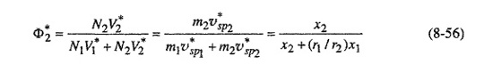
where m_i is the mass of component i in the mixture, is the characteristic specific volume and χ_i = N_i/N is the mole fraction.

Assuming random mixing of surface contacts between molecules, the energy of the mixture is given by

(8-57)

where A_ij is the number of i-j contacts; each contact is characterized by the energy –η_ij/ν. From definitions given above [see Eq. (8-42)], it follows that

(8-58)

(8-59)

For a random mixture,

(8-60)

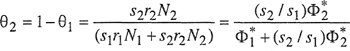
where the surface fractions θ₁ and θ₁ are defined by

(8-61)

Substitution of Eqs. (8-58) to (8-61) into Eq. (8-57) gives

(8-62)

where

(8-63)

and

(8-64)

By analogy with the energy for a pure component, we define for the mixture

(8-65)

Comparison of this equation with Eqs. (8-46) and (8-62) gives

(8-66)

where X₁₂ is an interaction parameter defined by²⁶

²⁶ Note that

(8-67)

Parameter X₁₂ is analogous to interchange energy w of Eq. (7-71), but X₁₂ has dimensions of energy density instead of energy.

Since Eq. (8-47) applies also to the mixture, with the aid of Eq. (8-55), we obtain

(8-68)

The partition function for the mixture [Eq. (8-52)] has the same form as that for a pure liquid. We assume that the combinatorial factor is independent of volume and temperature and that the “equation of state” (or residual) part, does not depend on the detailed structure of the fluid. The equation of state for the mixture, therefore, is identical to Eq. (8-45). However, reduced variables = P/P* and of the mixture depend on composition, as specified by Eqs. (8-66) and (8-68).

The thermodynamic properties of the mixture are directly related to the partition function²⁷ and can be calculated using Eq. (8-52). Pure-component properties are obtained in the same way from the partition function, either with N₁ = 0 or N₂ = 0. Thermodynamic mixing properties can now be calculated in the usual way. For example, the entropy of mixing, Δ_mixS follows as the sum of two contributions,

²⁷ See Table B-1 in App. B.

(8-69)

where superscripts C and R stand for combinatorial and residual, respectively.

The combinatorial contribution ΔS^C arises from combinatorial factor . The residual contribution S^R follows from the “equation-of-state” part of the partition function, determined by differences in intermolecular forces and free volumes. Because is assumed independent of volume and temperature, no combinatorial contribution appears in the enthalpy or in the volume of mixing.

Section 8.2 indicates that it is convenient to split mixing functions into a combinatorial part and a residual part, and allows a choice of several analytical expressions for ΔS^C, the combinatorial contribution to the entropy of mixing. The partition function presented here gives a residual contribution S^R, arising from differences between the equation-of-state parameters for the pure components (Flory, 1970):

(8-70)

For the enthalpy of mixing (or excess enthalpy H^E), we obtain

(8-71)

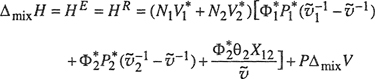
where the volume of mixing Δ_mixV (or excess volume V^E) is given by

(8-72)

For a condensed phase at normal (low) pressure, the term PΔ_mixV is negligible; therefore, at low pressure, we may ignore the distinction between enthalpy and internal energy.

The residual Gibbs energy G^R is obtained by combining Eqs. (8-70) and (8-71):

(8-73)

From the residual Gibbs energy, we can obtain the activity of component 1. To do so, we redefine N₁ and N₂ to represent numbers of moles. If denotes the molar hard-core volume of the solvent (component 1), from Eq. (8-73) the residual part of the activity is

(8-74)

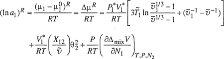
where at normal pressures the last term is negligible.

It is useful to compare (ln a₁)^R, given by Eq. (8-74) and neglecting the last term, with the semiempirical part for (ln a₁)^R used in the Flory-Huggins theory (Sec. 8.2). In Eq. (8-11) the residual part is given by

(8-75)

where χ is the Flory-Huggins interaction parameter. We relate Eq. (8-75) to Eq. (8-74) through identification of χ as the reduced residual chemical potential defined by

(8-76)

Contrary to the simple Flory-Huggins theory discussed in Sec. 8.2, χ now varies with composition, as found experimentally.

As formulated above, the Prigogine-Flory-Patterson theory is applicable to solutions of small molecules as well as to polymer solutions. The influence of liquid-state properties on each of the thermodynamic functions H^R, V^R, S^R, and is represented by “equation-of-state” terms that depend on the differences of reduced volumes (or their reciprocals) and on characteristic parameters P* and T*. These terms depend both on the difference between and and on the residual volume V^R through . In general, they do not vanish for V^E = 0. Thus the equation-of-state contributions cannot be interpreted simply in terms of a volume change upon mixing. The equation-of-state terms depend implicitly on X₁₂ through . Functions H^R (≡ H^E) and include a term that depends explicitly on χ₁₂; this term represents an enthalpy contribution that arises from nearest-neighbor interactions even when the mixing process is not accompanied by a volume change.

The Prigogine-Flory-Patterson theory of mixtures requires equation-of-state parameters ν*, T*, and P* for the pure components. In addition, two quantities are necessary for the characterization of a binary mixture: Segment surface ratio s₂/s₁ and parameter X₁₂ that reflects the energy change upon formation of contacts between unlike molecules (or segments). Both parameters can be chosen to match any two of the several possible experimental thermodynamic properties for the mixture. Because the segments of the two components are chosen to have the same core volume , the ratio s₂/s₁ is the ratio of the surfaces per unit core volume that can be estimated from structural data as tabulated, for example, by Bondi (1968). In that case, there remains the single parameter χ₁₂ to be assigned for a binary mixture. It may be chosen to optimize agreement between calculated and experimental enthalpies of mixing (or dilution) or volumes of mixing, because these properties are independent of the expression used for the combinatorial contribution.

Eichinger and Flory (1968), have investigated the system benzene/polyisobutylene at 25°C. They used experimental data for the volume of mixing, the enthalpy of mixing and solvent activities to test the theory. From structural information they estimated s₂/s₁ = 0.58, where subscript 2 refers to the polymer and subscript 1 to the solvent. The enthalpy data and the pure-component parameters from Tables 8-3 and 8-4 yield χ₁₂ = 41.8 J cm-³. With all parameters fixed, values of the reduced residual chemical potential χ were calculated from Eq. (8-74). Figure 8-13 shows the calculated results together with the experimental χ values obtained from solvent activity, using Eq. (8-11). Theory overestimates only slightly the effect of composition on χ.

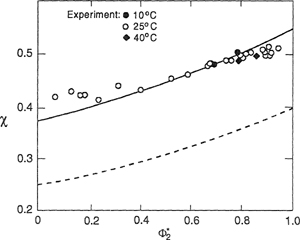
A modification of the residual chemical potential of the solvent [Eq. (8-74)] is made by appending the term analogous to X12, represents the entropy of interaction between unlike segments and is an entropic contribution to χ, the reduced residual chemical potential [Eq. (8-76)]. The appending term is independent of density and affects only the chemical potential and not the equation of state. If excess-volume data are used to determine X₁₂, the residual chemical potential of the solvent is under-predicted as shown by the dashed line in Fig. 8-14 for natural rubber and benzene (Eichinger and Flory, 1968a). By adjusting Q₁₂, a better representation of χ is obtained without affecting the representation of volumetric properties.

Calculated values of the excess volume, however, do not agree well with experimental data. Theory predicts positive values for V^E but calculated values are too large by a factor of about 2. The excess volume is quantitatively reproduced by theory only with a negative X₁₂. Thus the theory is not able to represent all excess functions with the same binary parameter.

Figure 8-13 Reduced residual chemical potential χ [Eq. (8-76)] of benzene (1) in polyisobutylene (2) at 25°C. Solid curve calculated from Eq. (8-74) with s₂/s₁ = 0.58 and X₁₂ = 41.8 J cm^-3 (Eichinger and Flory, 1968). The experimental χ was obtained from solvent-activity data using Eq. (8-11).

Figure 8-14 Reduced residual chemical potential χ of benzene (1) in natural rubber (2) at 25°C. Dashed curve calculated from Eq. (8-74) with s₂/s₁ = 0.90, X₁₂ = 5.86 J cm^-3, and Q₁₂ = 0. The solid line is calculated with same values of s₂/s₁ and X₁₂, and with Q₁₂ = -0.0184 J cm^-3 K^-1 (Eichinger and Flory, 1968a).

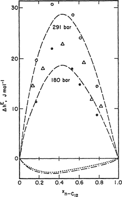
Another deficiency of the theory arises when X₁₂ is determined from data at various temperatures. Usually, X₁₂ decreases with increasing temperature. For example, Heintz (1977) found such a temperature dependence for cyclohexane/n-alkane systems. Heintz (1980) also showed that parameter X₁₂ depends on pressure when determined from h^E data at various pressures. The calculated composition dependence of h^E at various pressures is sensitive to variations in X₁₂. To illustrate, Fig. 8-15 shows the difference Δh^E = h^E(P bar) – h^E(1 bar) for n-dodecane/cyclohexane at 25°C and at 180 and 291 bar. The experimental data show that Δh^E increases with rising pressure. The dashed curves in the upper part of the figure are calculated using Eq. (8-71) with characteristic parameters from Table 8-3, ratio s₂/s₁ = 0.997, and X¹² adjusted to obtain best agreement. Values for X₁₂ are 13.5 and 14.0 J cm^-3 at 180 and 291 bar, respectively. If calculations at the higher pressures are performed with X₁₂ determined from h^E data at ambient pressure (X₁₂ = 12.9 J cm^-3), the results obtained are shown by the dotted (at 180 bar) and the dashed-dotted (at 291 bar) curves shown in the lower part of Fig. 8-15.

Figure 8-15 Effect of pressure on the excess enthalpy Δh^E [where Δh^E = h^E(P bar) –h^E(1 bar)] for the system n-dodecane/cyclohexane at 25°C. •, O Calorimetric data at 180 and 291 bar, respectively; Δ from volumetric data at 180 bar; – – – from Eq. (8-71) with X₁₂ adjusted at 180 bar (X₁₂ = 13.5 J cm^-3) and at 291 bar (X₁₂ = 14.0 J cm^-3); ······ (180 bar) and –·–·– (291 bar) from Eq. (8-71) with X₁₂ = 12.9 J cm^-3 obtained at 1 bar (Heintz and Lichtenthaler, 1980).

The quantity Δh^E is predicted poorly by the Prigogine-Flory-Patterson theory when the crucial parameter X₁₂ is determined from data obtained at ambient pressures. Heintz attempted to explain the pressure dependence of X₁₂ in terms of the orientational order in dense fluids containing long n-alkane chains. Using a statistical model for cooperative transitions, he developed an analytical expression for the dependence of X₁₂ on temperature and pressure. Incorporation of this model into the Prigogine-Flory-Patterson theory gives better agreement between theory and experiment for all systems investigated by Heintz.

While it is evident that Prigogine-Flory-Patterson theory has serious deficiencies, it can explain a phenomenon that has been observed for many polymer/solvent systems (Patterson, 1969, 1970): Partial miscibility at low temperatures and also at high temperatures.²⁸ The original Flory-Huggins theory can explain only partial irascibility at low temperatures.

²⁸ For a review, see J. M. Cowie, 1973, Ann. Rep. Chem. Soc. (Land.), 70A: 173.

We do not here go into details (given by Siow et al, 1972; Zeman and Patterson, 1972) but give only the essential argument. According to traditional Flory-Huggins theory, Flory parameter χ decreases slowly with rising temperature (Patterson, 1969, 1970), as indicated by the enthalpic contribution shown in Fig. 8-16, curve 2. In the traditional theory there is no entropic contribution to χ.

Figure 8-16 Temperature dependence of the χ parameter: curve 1, entropic contribution (due to free volume dissimilarity between polymer and solvent}; curve 2, enthalpic contribution (due to contact energy dissimilarity between polymer and solvent); curve 3, total χ.

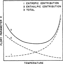
However, in the Prigogine-Flory-Patterson theory, free-volume (or equation-of-state) effects also contribute to χ. These are entropic contributions; they can be taken into account by parameter Q₁₂, as mentioned above. As temperature rises, the free volume of the solvent increases, especially as the temperature comes close to the critical of the solvent. However, the free volume of the polymer is nearly constant, increasing only slowly with rising temperature. Because the difference in free volumes increases with temperature, entropic contributions for χ rise with temperature, as indicated by curve 1 in Fig. 8-16. The total value of χ is given by the sum of the enthalpic and entropic contributions, indicated by the top line in Fig. 8-16. At low temperatures and at high temperatures, χ exceeds the limit for complete miscibility; at intermediate temperatures, χ is low enough for the mixture to be miscible in all proportions. The effect of temperature on χ, shown in Fig. 8-16, produces the phase diagram shown in Fig. 8-9(a). Such phase diagrams have been observed for a variety of polymer/solvent systems.

Figures 8-17 and 8-18 show experimental results for the system polystyrene/acetone. The tendency toward limited miscibility rises with the polymer’s molecular weight (Siow et al., 1972). Increasing pressure lowers the tendency toward partial miscibility (Zeman and Patterson, 1972), especially at high temperature, because rising pressure decreases the free-volume difference between the two components.

Figure 8-17 Phase diagram (temperature-volume fraction) for the polystyrene/acetone system for indicated polymer weight-average molecular weight (Siow etal., 1972).

Figure 8-18 Phase diagram (temperature-composition) for a polystyrene fraction of and for indicated pressures, in acetone (Zeman and Patterson, 1972). Results extrapolated from vapor-pressure data to 0 bar (Myrat and Rowlinson, 1965).

The Prigogine-Flory-Patterson theory has also been used to study the effect of compressibility on miscibility in polymer blends. McMaster (1973) used a generalized version of the Prigogine-Flory-Patterson equation of state to show qualitatively how differences in pure-component thermal-expansion coefficients can lead to lower-critical-solution-temperature (LCST) behavior in polymer blends. The effects of molecular weight, pressure and polydispersity were also considered qualitatively. Kammer et al. (1989) added a parameter reflecting differences in segment size and illustrated its effect on blend miscibility. In addition to differences in interaction energy and compressibility effects, UCSTs and LCSTs in polymer blends are sensitive to the segment-size parameter. Rostami and Walsh (1985) considered the effect of pressure and molecular weight on the UCST in polymer blends using the Prigogine-Flory-Patterson equation of state. Figure 8-19 illustrates that this equation of state gives reasonable prediction of the increase in UCST with pressure from atmospheric to 1013 bar for polybutadiene mixed with polystyrene using two binary parameters X₁₂ and Q₁₂. X₁₂ was determined from fitting experimental enthalpies of mixing and was the same for all molecular weights of either polymer. Q_l2, determined by fitting the maximum cloud-point temperature at atmospheric pressure, varied with the molecular weights of both polymers.

Figure 8-19 Experimental cloud points for polybutadiene (1)/polystyrene (2) blends at 1.013 bar (O) and 1013 bar (•). Binodals (——) and spinodals (– – –) are calculated at each pressure with the Prigogine-Fiory-Patterson equation of state with s₂/s₁ = 0.9, X₁₂ = 7.0 J cm^-3 and Q₁₂ = 0.0062 J cm^-3 K^-1 (Rostami and Walsh, 1985).

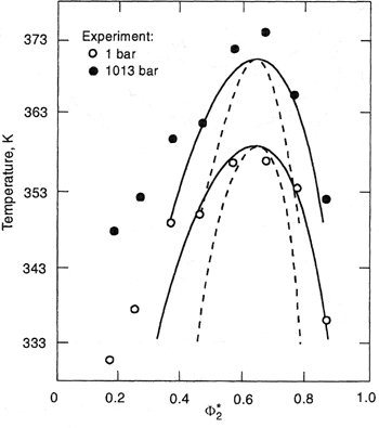
The Prigogine-Flory-Patterson theory corrects two major inadequacies of the conventional Flory-Huggins theory of polymer solutions: First, Flory-Huggins takes into account only the combinatorial entropy and contributions to the enthalpy due to nearest-neighbor interaction in a lattice framework (see Sec. 8.2). The Prigogine-Flory-Patterson theory considers, in addition, contributions to the entropy and enthalpy of mixing [Eq. (8-70)] that follow from differences in liquid-state properties of solute and solvent. This theory can explain negative enthalpies for mixtures of a polymer with a chemically similar solvent. The contribution from nearest-neighbor interactions in nonpolar mixtures is positive, though small; however, there may be large negative equation-of-state contributions. Negative enthalpies of mixing, often observed for polymer solutions, are thus explained (Flory et al., 1968) without invoking an implausible negative interaction parameter χ. Most important, Prigogine-Flory-Patterson theory is able to explain the frequently observed existence of a lower critical solution temperature in polymer/solvent systems that lies above the upper critical solution temperature. However, contrary to the original Flory-Huggins theory, the Prigogine-Flory-Patterson theory requires three parameters for each pure component.

These significant improvements are accomplished at considerable cost in algebraic complexity and need for pure-component parameters. Better agreement with experiment doubtless can be achieved with a more refined theory, but the improvement thus gained is likely to require additional binary parameters. An attractive feature of the Prigogine-Flory-Patterson theory is its straightforward extension to multicomponent mixtures (Pouchly and Patterson, 1976) requiring only pure-component and binary parameters.

It is important to remember that the Prigogine-Flory-Patterson theory is incorrect at low densities because, at low densities, Eq. (8-45) does not reduce to the equation of state for an ideal gas. Therefore, this theory is only applicable to fluids and fluid mixtures with liquid-like densities, i.e. liquids or fluids at very high pressures. However, the essential ideas of the Prigogine-Flory-Patterson theory can be generalized to the entire fluid-density range through perturbed hard-chain theory and its variations.

Perturbed-Hard-Chain Theory

The limitations of the Prigogine-Flory-Patterson theory at low densities have been removed by the perturbed-hard-chain (PHC) theory. The PHC equation of state and its essential features are presented in Sec. 7.16. Here we only briefly discuss its application to polymer solutions, in particular to the calculation of Henry’s constants.

Henry’s constant for volatile solute (1) in polymer (2) is defined by

(8-77)

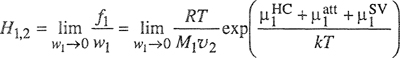
where f₁ is the fugacity and w₁ is the weight fraction of the volatile solute; M₁ is the molar mass of the solute, R is the gas constant, and ν₂ is the specific volume of the polymer. In Eq. (8-77), and are the chemical potentials from the hard-chain part, attractive part, and second-virial-coefficient part, as calculated from the PCH equation of state for mixtures (Kaul et al., 1980).

Ohzono et al. (1984) and Iwai and Arai (1991) applied the PHC equation of state to correlate weight-fraction Henry’s constants of hydrocarbon vapors in molten polymers. Figure 8-20 compares calculated and experimental Henry’s constants of normal alkanes in polypropylene. With one adjustable binary parameter, Henry’s constants are well correlated over a considerable range of temperature. The binary parameter pro-vides a small (but significant) correction to the geometric-mean assumption for calculating the energy of interaction between a solute molecule and a segment of a polymer molecule. Another, similar example is shown in Fig. 10-15.

Figure 8-20 Henry’s constants for n-alkanes in polypropylene. Points are experimental data and curves are calculated using the PHC equation of state (Iwai and Arai, 1991).

Lattice-Fluid Theory

The molecular lattice fluid (LF) theory for liquid and gaseous mixtures developed by Sanchez and Lacombe (1976, 1977, 1987) is formally similar to the Flory-Huggins theory discussed in Sec. 8.2. The essential and important difference is that LF theory includes empty lattice sites (holes). An equation of state characterizes each of the pure components as well as the mixture. Volume changes upon mixing are taken into account, as required for a good description of fluid-phase behavior.

The lattice is occupied by both r-mers and vacant lattice sites. For a pure component, the total number of lattice sites N_r is

(8-78)

where N₀ is the number of vacancies and N is the number of molecules, each with r segments. At closest packing, the volume of a molecule, assumed to be independent of temperature and pressure, is rν*, where ν* is the volume of a segment, equal to the volume of one lattice site. The total volume of the system is

(8-79)

where V now depends on temperature and pressure through N₀.

A reduced density is defined as the fraction of occupied sites,

(8-80)

where ρ = Nr/V is the density of segments, ν = V/Nr is the volume per segment, and is the reduced volume.

The energy of the lattice depends only on nearest-neighbor interactions. For a pure component, the only non-zero interaction energy is the mer-mer pair interaction energy ε. Vacancy-mer and vacancy-vacancy interactions energies are zero. The Sanchez-Lacombe model assumes random mixing of vacancies and mers; therefore, the number of mer-mer nearest-neighbors is proportional to the probability of finding two neighboring mers in the system. The lattice energy is

(8-81)

where z is the coordination number of the lattice.

The configurational partition function for this system is

(8-82)

The combinatorial factor Q^C is identical to that of the Flory-Huggins incompressible-lattice partition function where the solvent is replaced by a vacancy,

(8-83)

where the constant, r and N are independent of volume. However, N₀ depends on volume [Eq. (8-79)], and therefore Q^C contributes to the equation of state.

Substitution of Eqs. (8-81) and (8-83) into Eq. (8-82) and differentiation according to Eq. (7-209), yields the Sanchez-Lacombe lattice-fluid equation of state:

(8-84)

where the reduced (~) and characteristic (*) temperature and pressure are defined by

(8-85)

Characteristic parameters P*, υ*, and T* obey the equation

(8-86)

Reduced volume defined in Eq. (8-80) as the ratio of volume υ and close-packed volume υ* per segment, is also given by the ratio of the corresponding specific volumes υ_sp = 1/ρ_sp and where ρsp and are mass densities. Size parameter r in Eq. (8-84) is related to the mass of one molecule, m, and to by

(8-87)

A real fluid is characterized either by the three molecular parameters zε, υ* and r or by the three equation of state parameters, T*, P*, and . In principle, this equation of state is suitable for describing thermodynamic properties of fluids over an extended range of external conditions from the ordinary liquid or gaseous state to high temperatures and pressures where the fluid may be supercritical. To use the equation of state, we must know the characteristic parameters. In principle, any experimental configurational thermodynamic property can be used to determine these parameters. However, vapor-pressure data are particularly useful for solvents because they are readily available for a wide variety of fluids. For polymers, the characteristic parameters can be determined by a nonlinear least-square fit of experimental liquid density data over a range of pressures and temperatures. When only limited P-V-T data are available, the parameters can be estimated from experimental values of density, thermal expansion coefficient and compressibility at ambient temperature and pressure. Equation-of-state parameters for many fluids and liquid polymers have been reported by Sanchez and Panayiotou (1994).

Equation (8-84) shows that P-V-T data for polymer liquids are relatively insensitive to polymer molar mass. As polymer molecular weight increases, the 1/r term becomes insignificant. In the limit of infinite polymer molecular weight, Eq. (8-84) suggests a corresponding-state behavior for polymer liquids, illustrated in Fig.8-21. The lines for each reduced pressure were calculated using Eq. (8-84) in the limit r → ∞. The points are experimental P-V-T data for several polymers reduced by appropriate characteristic parameters. A reduced pressure = 0, is essentially atmospheric pressure; = 0.25 is a pressure of the order 1000 bar.

Figure 8-21 Corresponding-stales behavior of polymer P-V-T data according to the Sanchez-Lacombe equation of state Points are experimental data and lines are calculated from Eq. (8-84) in the limit r → ∞. PS, polystyrene; PoMS, poly(o-methyl styrene); PcHMA, poly(cyclohexyl methacrylate); PMMA, poly(methyl methacrylate); PnBMA, poly(n-butyl methacrylate); LDPE, low-density polyethylene; PIB, polyisobutylene; PVAc, poly(vinyl acetate); PDMS, poly(dimethyl siloxane); PRO, poly(propylene oxide) (Sanchez and Lacombe, 1978).

To extend the lattice fluid theory to mixtures, we need appropriate mixing rules for the characteristic parameters. There is a fundamental difficulty here because the segment size of any one component is not necessarily equal to that of another component. Each pure component has its own volume per segment. In a lattice model, how do we mix segments of different size? Some assumptions are required. The original formulation of the lattice-fluid equation of state for mixtures (Sanchez and Lacombe, 1976, 1978) uses assumptions similar to those used in the Prigogine-Flory-Patterson equation of state. First, the molecular volume of each component is conserved: the molecular volume of a component, determined from its pure-fluid properties is equal to its molecular volume in the mixture Consequently, the chain length of a component in the mixture, r_i, may differ from that for the pure fluid, . In addition, the total number of pair interactions in the close-packed mixture is equal to the number of pair interactions of the pure components in their close-packed states. Because the Sanchez-Lacombe equation of state assumes random mixing of segments, these assumptions lead to

(8-88)

(8-89)

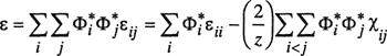
where the segment fraction²⁹ is

²⁹ Sanchez and Lacombe (1978) use close-packed volume fraction, by definition equal to the segment fraction in this chapter.

(8-90)

and 2χ_ij / z = (ε_ii + ε_jj – 2ε_ij)/kT is the interaction parameter in terms of the interchange energy [Eq. (7-71)]. ε_ij (or equivalently χ_ij/z) is an adjustable binary parameter.

With υ* and ε defined by Eqs. (8-88) and (8-89), Eqs. (8-80) and (8-85) define characteristic quantities P* and T* for the mixture. The equation of state for the mixture is identical to Eq. (8-84); however, r, explicit in Eq. (8-84), becomes an average value for the mixture, given by

(8-91)

Parameter characterizes a binary mixture; all other parameters are related to those of the pure components. Alternatively, the characteristic pressure of a binary mixture can be expressed in terms of pure-component characteristic quantities as:

(8-92)

Parameter is equivalent to parameter χ₁₂ in the Prigogine-Flory-Patterson theory [Eq. (8-67)] and has dimensions of energy density. Parameter χ₁₂ provides a measure of the energy change upon formation of contacts between unlike molecules (or seg-ments).

Because the mixing rule for υ* is somewhat arbitrary, a common alternative to Eq. (8-88) is

(8-93)

where and provides a second binary parameter. Other approximations can be used to count the number of pair interactions. For example, we can assume random mixing of contact sites rather than random mixing of segments (Panayiotou and Vera, 1981, 1982), as well as non-random mixing (Panayiotou and Vera, 1982; Panayiotou 1987), but ε_ij typically remains the essential binary parameter.

The lattice-fluid model, summarized above, is applicable to solutions of small molecules as well as to polymer solutions. Like the Prigogine-Flory-Patterson equation of state, the lattice-fluid model and its variations have been used to correlate the composition dependence of the Flory parameter χ (residual chemical potential of solvent) (Panayiotou and Vera, 1982; Panayiotou 1987). These studies show that a binary entropic-interaction parameter (analogous to the Q₁₂ parameter in the Prigogine-Flory-Patterson equation of state) is also needed to provide better agreement with measured residual chemical potentials for the solvent.

The essentials of liquid-liquid miscibility are obtained by studying the spinodal condition. According to the lattice-fluid equation of state, immiscibility occurs when the following inequality holds (Sanchez and Lacombe, 1978):

(8-94)

where

(8-95)

and κ_T is the isothermal compressibility of the mixture:

(8-96)

In Eq. (8-94), the first bracketed term is the combinatorial-entropy contribution; is an energetic contribution and is an entropic contribution from the equation of state. Figure 8-22 illustrates the general behavior of these three terms as a function of temperature. The last term makes an unfavorable contribution to the spinodal and favors demixing. Its magnitude increases with increasing temperature and diverges as the vapor-liquid critical temperature T_c is approached, because K_T → ∞ as T → T_c. Hence, according to the lattice-fluid theory, every polymer solution in equilibrium with its vapor should exhibit a LCST prior to reaching its liquid-vapor critical temperature.

Figure 8-22 Schematic behavior of the three terms in the spinodal inequality [Eq. (894)] from the lattice-fluid equation of state as a function of temperature (Sanchez and Lacombe, 1978). The horizontal line represents the combinatorial contribution. The dotted-dashed curve is the sum of the energetic contribution and the entropic contribution. When this sum lies below the combinatorial contribution, the polymer and solvent are miscible. When the sum lies above the combinatorial contribution, the mixture will phase separate. Intersections of the dotted-dashed curve and horizontal Sine represent upper (UCST) and lower (LCST) critical solution temperatures. T_c is the vapor-liquid critical temperature of the polymer solution.

The lattice-fluid model and its modifications have been successfully used to represent thermodynamic excess properties, vapor-liquid and vapor-liquid-liquid equilibria for a variety of mixtures, as summarized by Sanchez and Panayiotou (1994).

Kim and Paul (1992) investigated the phase behavior of polymer blends containing polycarbonates. Blends of polystyrene (PS) and tetramethyl bisphenol-A polycarbonate (TMPC) show phase separation at temperatures above about 240°C depending on the composition of the blend. The characteristic parameters for PS and TMPC in Table 8-6 were obtained by a non-linear regression fit of Eq. (8-84) to experimental volumetric data in the pressure and temperature ranges 0-500 bar and 220-270°C. The latter includes the range where phase separation of PS/TMPC blends has been observed. Using the pure-component parameters in Table 8-6, an interaction-energy parameter was obtained from the phase-separation data. was assumed independent of temperature and was found to be independent of blend composition.

Table 8-6 PS and TMPC* parameters for the Sanchez-Lacombe equation of state (Kim and Paul, 1992).

Figure 8-23 shows the calculated spinodal curve together with experimental phase-separation temperatures obtained by differential scanning calorimetry. The solid line calculated with agrees well with experiment.

Figure 8-23 Comparison of experimental phase separation temperatures () obtained by differential scanning calorimetry with the spinodal curve (—) predicted by the lattice-fluid model (Kim and Paul, 1992).

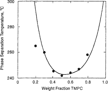
In addition to mixtures of polymers with normal solvents, the lattice-fluid equation of state has also been applied to polymer-gas systems. Sanchez and Rodgers (1990, 1993) used it to predict gas solubility at infinite dilution. The physical properties of the gas and polymer dominate gas solubility and the gas-polymer interaction plays a secondary role. Using no adjustable parameters, gas solubility was quantitatively predicted for several hydrocarbons and chlorinated hydrocarbons in nonpolar polymers such as polystyrene, poly(1-butene) and atactic polypropylene. For polar polymers, such as poly(vinyl acetate) and poly(methyl methacrylate), the solubilities of hydrocarbons were greatly overestimated, but polar and aromatic gases were correlated reasonably well. Similarly, Pope et al. (1991) attempted to predict sorption isotherms of nitrogen, methane, carbon dioxide, and ethylene in silicone rubber. Model parameters were determined only from pure-fluid properties without using any mixture data. Figure 8-24 shows a typical isotherm for ethylene. In general, the experimental isotherm in underpredicted. From the equation of state, expressions for the partial molar volumes and Henry’s constant at infinite dilution for the gases can be derived. In general, the Henry’s constant is underpredicted, but a good estimate of the partial molar volume at infinite dilution was obtained.

Figure 8-24 Comparison of experimental and theoretical results using Sanchez-Lacombe equation of state (no adjustable parameters) for ethylene sorption in silicone rubber (Pope et al., 1991).

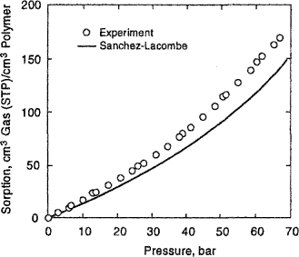
Another application of the lattice-fluid equation of state is provided by describing the effect of a compressed-gas diluent on the behavior of a glassy polymer (Wissinger and Paulaitis, 1991; Condo et al., 1992; Condo and Johnston, 1992; Kalospiros and Paulaitis, 1994). Compressed gases can act as plasticizers when dissolved in a glassy polymer matrix by lowering the polymer’s glass-transition temperature (T_g). The glass transition of a polymer or polymer/diluent mixture can be determined by using the Gibbs-Di Marzio criterion (1958, 1963). This criterion states that, at the glass transition, the polymer is essentially “frozen” and has zero configurational entropy. The sorption of the compressed fluid by the polymer and T_g can be calculated simultaneously by solving the equation of state, the condition of equilibrium for partitioning of the diluent between the polymer and the gas phase, and the Gibbs-Di Marzio criterion. Figure 8-25 shows results for poly(methyl methacrylate) (PMMA)/CO₂. Figure 8-25(a) illustrates good agreement between experimental and calculated T_g depression as a function of concentration of dissolved CO₂. However, Fig. 8-25(b), a plot of T_g against CO₂ pressure shows unexpected phase behavior, first discovered with the model. This unexpected phase behavior is called retrograde vitrification (by analogy with retrograde condensation - see Sec. 12.2). For example, at 373 K and a CO₂ pressure of 30 bar, the polymer is a liquid. Decreasing the temperature causes the polymer to undergo a liquid-to-glass transition, as expected; however, a further decrease in temperature causes the glass to become a liquid again. This effect results from the competition between polymer-segment mobility that declines with falling temperature, and diluent solubility that increases with falling temperature.

Figure 8-25 (a) Calculated (——from lattice-fluid theory) and experimental (ο, Wissinger and Paulaitis, 1991 a; Chiou ef al., 1985) glass-transition depression of PMMA as a function of CO₂ solubility, (b) Glass-transition temperature depression of PMMA as a function of CO₂ pressure showing retrograde vitrification behavior (Condo et al., 1992). —— Calculated from lattice-fluid theory; o, experiment (Wissinger and Paulaitis, 1991a).

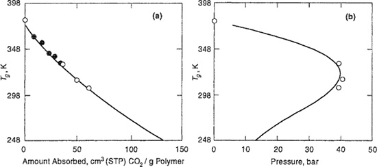
The lattice-fluid equation of state has also been used to describe the phase behavior of supercritical fluid-polymer systems. In these systems, the polymer may completely dissolve in the supercritical-fluid phase, or partition between a polymer-rich phase and a supercritical fluid-rich phase. Figure 8-26 shows an example: poly(ethykne glycol) (PEG, M = 400 g mol^-1) mixed with CO₂ to pressures of approximately 260 bar at 50°C (Daneshvar et al, 1990). The upper curve (left-hand axis) gives the weight fraction of CO₂ dissolved in the polymer-rich phase and the lower curve (right-hand axis) gives the weight fraction of polymer dissolved in the super-critical fluid-rich phase. The curves are calculated using the random-mixing version of the lattice-fluid model (Panayiotou, 1987) with one adjustable binary parameter.

Figure 8-26 Compositions of coexisting phases for PEG/supercritical CO₂ mixtures at 323 K as a function of pressure.— Calculated from the Panayiotou-Vera version of the lattice-fluid equation of state; , O experiment (Daneshvar et al., 1990).

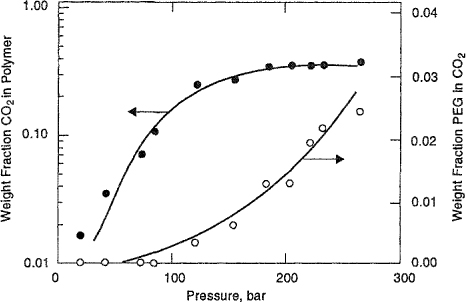
The lattice-fluid theory has also been modified to account for strong interactions (hydrogen bonding) between polymer and solvent. This modification has been successfully tested with experimental data for vapor pressures, enthalpies and volumes of mixing for chloroform/polyether solutions (Panayiotou and Sanchez, 1991). The essential features of this modification are discussed by Sanchez and Panayiotou (1994).

Statistical Associated Fluid Theory

The statistical associated-fluid theory (SAFT), introduced in Sec. 7.17, has successfully been applied to correlate thermodynamic properties and phase behavior of pure liquid polymers and polymer solutions, including the solubility of gases in polymers, supercritical and near-critical solutions. For example, Wu and Chen (1994) investigated gas solubility in polyethylene. Figure 8-27 shows a comparison of experimental and calculated solubilities of methane and nitrogen in polyethylene using the SAFT equation of state. In their calculations, Wu and Chen used a generalized binary parameter correlation that depends on temperature. Even at very high pressures (600 bar), the agreement between experiment and SAFT is very good.

Figure 8-27 Solubilities of methane and nitrogen in polyethylene at 461.4 K. , ο experiment. —— Calculated from SAFT equation of state. The binary parameter is calculated from a temperature-dependent correlation (Wu and Chen, 1994).

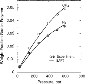
Numerous applications of the SAFT equation of state to supercritical and near-critical solutions of polymers have been published (Chen and Radosz, 1992; Gregg et al., 1993; Chen et al., 1992, 1993, 1994, 1995; Condo and Radosz, 1996; Banaszak et al., 1996). Figure 8-28 shows experimental and calculated pressure-temperature cloud-point curves for alternating poly(ethylene-propylene) (PEP)/propylene for different PEP molecular weights (Chen and Radosz, 1992). The SAFT equation of state can correlate the experimental data with one binary parameter k_ij that depends on, and can be correlated with polymer molecular weight. Figure 8-28 also shows predictions for propylene with PEP (_w = 10,000 and 15,000 g mol^-1) using the same empirical correlation for k_ij. As shown in the insert of Fig. 8-28, as the polymer molecular weight increases, the LCST curve is shifted to lower temperatures and, simultaneously, the UCST curve is shifted to higher temperatures, i.e., the two curves approach each other and eventually merge into a single curve with a minimum. (This single curve is represented in the insert by a dashed-dotted line.) This behavior is illustrated in the figure with the data for the real system. Calculations from SAFT show that, for propylene/PEP with _w = 10,000 g mol^-1 (or larger), the LCST and UCST curves have merged, as confirmed by experiment.

Figure 8-28 Experimental (Chen and Radosz, 1992) and calculated P-T phase boundaries for alternating poly(ethylene-propylene) (PEP)/propylene for the indicated PEP molecular weights. Calculations use the binary interaction-parameter correlation developed for this system. For the propylene/PEP (_w = 10,000 g mol^-1) system, SAFT predicts a steep upper critical solution temperature (UCST) with an upper critical end point (UCEP) near -80°C. (Chen et al., 1992). Experiment; —calculated from SAFT equation of state. The insert shows schematically the influence of increasing polymer molecular weight (represented by the arrow) in the P-T diagram. In the insert, the heavy line is the bubble-point curve; in most cases, this curve coincides with the vapor-pressure curve of the solvent.

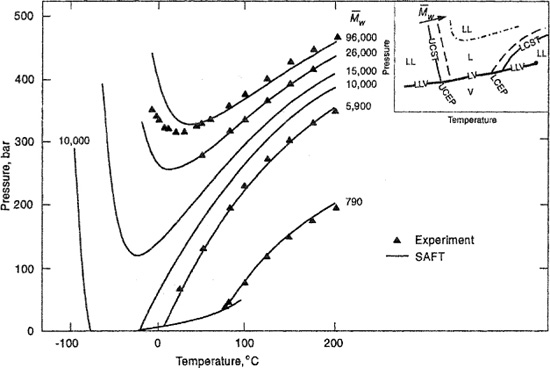
Perturbed Hard-Sphere-Chain Theory

The perturbed hard-sphere-chain (PHSC) equation of state introduced in Sec. 7.17 can represent all common types of fluid phase diagrams of binary polymer mixtures including vapor-liquid equilibrium³⁰ (Gupta, 1995, 1996) and, for some cases, liquid-liquid equilibrium (Song et al., 1994a). However, good representation of liquid-liquid equilibria is much more difficult than representation of vapor-liquid equilibria; existing theories usually require two or three binary parameters as pointed out by Hino (1996).

³⁰ A comprehensive collection of vapor-liquid equilibria data for binary polymer solutions is presented by Ch. Wohlfarth, 1994, Vapor-liquid Equilibrium Data of Binary Polymer Solutions, Physical Sciences Data Series No. 44. Amsterdam: Elsevier.

Gupta (1996) showed that vapor-liquid equilibrium of polymer solutions can be correlated quantitatively with the PHSC equation of state. However, for accurate results, Gupta relaxed the hard-sphere additivity rule for calculating b_ij to introduce a binary size parameter λ_ij;

(8-97)

where

(8-98)

Therefore, a binary solution has two adjustable parameters: k_ij for the energy parameter [Eq. (7-260)] and λ_ij for the size parameter. As an example, Fig. 8-29 shows a comparison of theory and experiment for the chloroform/polystyrene (PS) system. The binary size interaction parameter λ_ij was adjusted at 50°C and then prediction was made at 25°C. In this calculation, the binary energy interaction parameter, k_ij, was set equal to zero. Results similar to those shown in Fig. 8-29 were obtained for many other binary systems. Calculated results are strongly sensitive to λ_ij. Even a small value (|λ_ij|<<1) can have a large effect on the calculated equilibria. Gupta (1995) has also presented calculated and observed vapor-liquid equilibria for random copolymers.

Figure 8-29 Vapor-liquid equilibrium for chloroform/polystyrene [_n(PS) = 290,000 g mol^-1] solutions (Gupta. 1996). , ο Experiment. Curves are fitted (—) and predicted (- - -) from PHSC equation of state. Experimental data at 50°C were used to determine the binary parameter λ_ij = -0.0234 (k_ij was set equal to zero).

Quantitative representation of vapor-liquid equilibria for real polymer systems can be achieved even by cubic equations of state, as shown by Tassios and coworkers (Kontogeorgis et al., 1994; Harismiadis et al., 1994). However, a much more stringent test for any equation of state is quantitative representation of liquid-liquid equilibria. Lambert et al. (1995) and Hino et al. (1995) have shown that the PHSC equation of state can quantitatively correlate liquid-liquid equilibria of binary and ternary (one polymer and two solvents) systems exhibiting both an upper (UCST) and lower (LCST) critical solution temperatures. However, quantitative representation of polymer-solvent liquid-liquid equilibrium is not possible when pure-component parameters for the polymer are obtained from P-V-T data only. To represent such equilibria it is necessary to use some mixture property to obtain pure-component polymer parameters (Lambert et al., 1995). This is necessary because, at present, no single theory is able to describe correctly the properties of a polymer in both the pure molten state and in the highly dilute solution state. Therefore, characteristic polymer parameters obtained from pure-polymer data are not meaningful when the polymer is in a dilute solution.

Hino et al. (1994, 1995) used the PHSC equation of state to calculate coexistence curves and miscibility gaps for blends, that is, polymer mixtures of homopolymers and homopolymer/copolymer systems. For polymer blends, existing theory is much better than for dilute solutions of a polymer in a common solvent. Figure 8-30 shows a comparison of calculated UCST coexistence curves with experimental data for polystyrene (PS)/polybutadiene (PBD) blends. Binary parameters k₁₂ and λ₁₂ were determined by matching the experimental UCST (Park and Roe, 1991) with that calculated at _n(PS) = 1,900 g mol^-1. Although the width of the calculated coexistence curve is narrower than that from experiment, the coexistence curves for the blends with _n(PS) = 2,220 and 3,300 g mol^-1 are reasonably predicted using the same binary parameters. These results indicate that the molecular weight dependence of UCST is predicted by the model. However, the width of the coexistence curve is always narrower than that from experiment, in particular at temperatures far below UCST. The model gives only semi-quantitative agreement with experiment. Similar results were obtained for systems where immiscibility is caused by LCST behavior (Hino et al., 1994).

Figure 8-30 Phase diagrams for polybutadiene [_n (PBD) = 2,350 g mol^-1]/polystyrene (PS) blends, (a) PBD/PS ( = 1,900 g mol^-1). (b) PBD/PS (_n = 2,220 g mol^-1) and PBD/PS (_n = 3,300 g mol^-1). Curves from the PHSC equation of state with k_ij = 0.00544 and λ_ij = 0.00117. In (b), curves are predicted. Experiment: ο Park and Roe (1991); , Roe and Zin (1980). Although k_ij and λ_ij are much smaller than unity, they significantly influence calculated phase diagrams.

8.4 Nonporous Polymeric Membranes and Polymer Gels

Polymer swelling occurs when polymeric materials are exposed to solvent vapors or gases that can be absorbed by the polymer. Swelling also occurs when cross-linked polymers (polymeric networks) that cannot be dissolved, are in contact with a compatible liquid. The important technical issue often is how fast (determined by diffusion) a low molecular-weight fluid is absorbed by a polymer. Applications where sorption behavior (solubility and diffusivity) is important are, for example, the use of supercritical fluids as swelling agents for impregnating chemical additives (e.g. dyes or pigments for color) into polymers (Berens et al., 1992) and, conversely, for extracting low molecular-weight components from polymeric materials (Cotton et al., 1993) or the separation of gaseous and liquid mixtures using selective nonporous polymeric membranes (Noble and Stern, 1995; Mulder, 1996).

Swelling properties of gels are also of considerable interest for applications in packaging and medicine (e.g. implants in eye surgery). Gels are three-dimensional cross-linked elastic polymers that may either swell or shrink when brought into contact with a liquid. Gels have been proposed as size selective extraction solvents and as environmentally sensitive permeability barriers for a variety of pharmacological agents (DeRossi et al., 1991; Dušek, 1993).

There are numerous aspects of polymer swelling. Here we focus only on the thermodynamics relevant for separation techniques using nonporous membranes and on phase behavior for systems containing gels. The thermodynamics discussed here may be useful for optimum design of membrane separation processes and for design of gels in medicine, pharmaceutics and biotechnology.

Nonporous Membranes

Most nonporous membranes used in industrial applications are composite membranes³¹ consisting of a thin, nonporous, polymeric top layer (thickness 0.5-5 μm) covering the surface of a porous support (thickness 100-500 μm). The thin top layer is mainly responsible for the separation. The support has usually no or little influence on the separation characteristics of the composite membranes. Its purpose is to provide mechanical stability in a membrane-separation unit (module).

³¹ A review on thin-film composite membranes is given by R. J. Petersen, 1993, J. Membrane Sci, 83: 81.

The separation mechanism of a nonporous membrane is illustrated in Fig. 8-31 for a binary fluid mixture, with different molecules represented by black and white spheres. The feed mixture to be separated flows along one side of the membrane while the two feed components are permeating into and through the membrane at different rates. Therefore, the retentate leaving the process on the same side of the membrane where the feed enters, is depleted in the component permeating preferentially. Consequently, the permeate collected on the other side of the membrane is enriched in the preferentially permeating component.

Figure 8-31 Schematic representation of a membrane-separation process using a composite membrane with a thin dense nonporous top layer and a thick porous support layer.

The driving force for any permeating component i is μ_i(feed) -μ_i(permeate) where μ is the chemical potential. This difference in chemical potentials is usually achieved by a permeate pressure much lower than the feed pressure. The resulting driving force causes each component to permeate with an individual velocity from the feed to the permeate. Therefore, at steady state, the compositions of the feed and permeate differ from each other. If the feed Is a liquid under its saturation pressure and the permeate is a vapor kept at low pressure (5-20 mbar) by using a vacuum pump combined with a cooling trap for condensing the permeate, the separation process is called pervaporation (Feng and Huang, 1997). If both feed and permeate are vapors or gases, the separation process is called vapor permeation or membrane gas separation.³² In this case, pressures applied on the feed side are 10-100 bar while the permeate pressure is 1 bar or less. If both feed and permeate are liquid and a pressure in the range 80-100 bar is applied on the feed side while the permeate is kept at ambient pressure, the separation process is called reverse osmosis (Amjad, 1993). Reverse osmosis is mainly applied to dilute aqueous solutions to produce purified water or to concentrate aqueous solutions by removing water.

³² A comprehensive review of membrane-based gas separations is given by W. J. Koros and G. K. Fleming, 1993, J. Membrane Sci, 83: 1.

Membrane materials used for the top layer can be divided into two main classes: hydrophilic and organophilic. Hydrophilic membranes are used, for example, in the separation of water from organic mixtures by pervaporation (Huang, 1991), drying of humid gas streams by gas separation or in the production of drinking water from seawater by reverse osmosis. Typical separations using organophilic membranes are removal of organic pollutants from water by pervaporation (Böddeker and Bengtson, 1991) and extraction of aroma compounds from alcoholic beverages by pervaporation (Baudot and Marin, 1997). Some synthetic membrane polymers have particular selectivities for aromatic hydrocarbons to separate them from aliphatic hydrocarbons (Inui et al, 1997; Yoshikawa et al., 1997) or for alcohols to separate them from ethers (Streicher et al., 1995; Nguyen et al., 1997) by pervaporation.

Other important membrane-separation processes include dialysis (particularly hemodialysis) and micro-, ultra- and nanofiltration using porous membranes; liquid membranes; and electrodialysis where charged membranes are used (Mulder, 1996). We do not discuss these processes here; we restrict our discussion to thermodynamics relevant to pervaporation, gas separation and reverse osmosis.

The driving force for any species permeating is the gradient of the species’ chemical potential across the membrane. Therefore, to determine the driving forces for various species we need the chemical potential for each species at state conditions of the feed and the permeate. We consider first a liquid mixture in equilibrium with its vapor. The condition for equilibrium is:

(8-99)

where μ_i^0G is the standard-state (1 bar) chemical potential of the pure gas, φ_i is the fugacity coefficient, P_i is the partial pressure, μ_i^0L is the chemical potential of the pure liquid at the same temperature and pressure as those of the mixture, γ_i^L is the activity coefficient, and x_i^L is the mole fraction of i in the liquid mixture.

For the liquid mixture in equilibrium with the swollen polymer, the condition for equilibrium is

(8-100)

with

(8-101)

where superscript M indicates the membrane phase. Because the standard state chemical potentials for the liquid phase, μ_i^0L, and for the membrane phase, μ_i^0M, are identical,

(8-102)

It is convenient to use molar concentration c_i^M in the membrane phase instead of mole fraction x_i^M; therefore, we rewrite Eq. (8-102)

(8-103)

Activity coefficient γ_i^c,M is based on molar concentration instead of mole fraction. From Eq. (8-103), we obtain

(8-104)

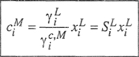
where S_i^L is the liquid solubility coefficient of component i.

Phase equilibrium between the gaseous (vapor) phase and the membrane phase requires

(8-105)

From Eqs. (8-99) and (8-103) we obtain

(8-106)

or

(8-107)

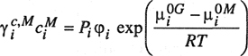
or

(8-108)

where the gas solubility coefficient of component i is

(8-109)

These equations are useful for the description of transmembrane fluxes within the framework of the solution-diffusion model. In this model, the transport of each component i is divided into three steps:

1. The components of the liquid or gaseous feed mixture are absorbed in the membrane. For each component i, there is thermodynamic solubility equilibrium at the phase boundary between the feed mixture and the membrane according to Eqs. (8-104) and (8-108).

2. The absorbed components diffuse across the membrane from the feed side to the permeate side according to Fick’s first law of diffusion.

3. The components are desorbed at the phase boundary between the membrane and the liquid or gaseous permeate. Again, it is assumed that for each component i, there is equilibrium at the phase boundary.

We consider first the case of pervaporation. Inside the membrane, flux J_i of component i is given by Fick’s law:

(8-110)

where D_i is the diffusion coefficient (with units m² s^-1 with J_i in mol m^-2 s^-1), and is the length coordinate perpendicular to the top layer of the membrane with thickness δ_M (0 ≤ ≤ δ_M). Integration of Eq. (8-110) (Heintz and Stephan, 1994) gives

(8-111)

where c^M_iF and c^M_iP are the concentrations (in mol m^-3) in the membrane boundaries at the feed side (index F) and the permeate side (index P), respectively. Equation (8-111) is valid only if D_i is independent of concentration; otherwise, D_i is the diffusion coefficient averaged over the concentration across the membrane.

According to the solution-diffusion model, the solubility equilibrium conditions at both phase boundaries justify substitution of c^M_iF from Eq. (8-104) and c^M_iP from Eq. (8-108) into Eq. (8-111):

(8-112)

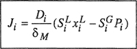
At steady state, the mole fraction y_i of the gaseous permeate is obtained from

(8-113)

For a binary mixture, substitution of Eq. (8-112) into (8-113) gives

(8-114)

Because P₂ = P – P₁, where P is the total pressure of the permeate, P₁ can be calculated from Eq. (8-114) at given values of x^L₂ = 1 – x^L₁ and P. Therefore, y₁ is also determined. If the pressure P in the permeate side is kept as low as possible, i.e., P ≈ 0, then also P_i ≈ 0. Equation (8-114) then simplifies to

(8-115)

A plot of the permeate mole fraction y₁ against liquid-feed mole fraction x₁^L according to Eq. (8-114) or (8-115) is called a separation diagram. A measure for the separation effect is the separation factor defined in terms of the upstream and downstream mole fractions x₁^L and y₁, respectively:

(8-116)

If the permeate pressure P ≈ 0, Eq. (8-115) gives

(8-117)

where product D_iS_i^L is called the permeability of component i. Figure 8-32 shows a separation diagram, y₁(x₁^L), for different values of α. If α is larger than 1, component 2 is enriched in the permeate; if α = 1, no separation effect is observed; if α is smaller than unity, component 1 is enriched in the permeate.

Figure 8-32 Separation diagram in pervaporation calculated from Eq. (8-115) for different values of the separation factor α.

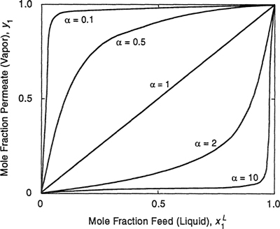
The equations derived above are only valid over the whole range of liquid composition if and are constants independent of the mixture composition. If and are functions of and y_i, respectively, the shape of the separation diagrams can become more complicated; in extremely nonideal cases, curves with a maximum or a minimum can be obtained. Further complications arise if the diffusive fluxes J_i are no longer independent of each other and diffusion coupling occurs.³³

³³ For a discussion and quantitative of these more complex cases, see Heintz and Stephan (1994)

In gas separation,³⁴ the flux J_i inside the membrane is also given by Eq. (8-111), with and from Eq. (8-108):

³⁴ More detailed information on gas separation is given by Koros and Fleming (1993) and Malder (1996).

(8-118)

where P_iF and P_iP are, respectively, the partial pressure of component i in the pressurized gaseous feed mixture (index F) and in the permeate mixture (index P).

Equation (8-109) shows that and depend on γ_i^c,M and φ_i. Both quantities are in principle concentration dependent; in particular, φ_i can change significantly with pressure. Therefore, and can differ from each other. However, often it is assumed that ≈ = . In this case, Eq. (8-118) simplifies to

(8-119)

As in pervaporation, we obtain a separation diagram that corresponds to Eq. (8-114), with substituted by y_iF = P_iF / ∑P_iF and y_iP = P_ip / ∑ P_iP. For the simplified case where P_iP <<P_iF, we obtain for a binary mixture an equation that is analogous to Eq. (8-115):

(8-120)

and the corresponding separation factor is defined by

(8-121)

As in pervaporation, is called permeability. In gas separation, special units are used. Flux J_i is expressed ³⁵ in m³ (STP) m^-2 s^-1 instead of mol m^-2 s^-1. Solubility coefficient is usually given in m³ (STP) m^-3 Pa^-1 and the diffusion coefficient is given in its SI-units, m² s^-1. The common unit for permeability is the barrer [1 barrer = 10^-10 cm³ (STP) cm cm^-2 s^-1 cmHg^-1 = 0.76x10^-17 m³ (STP) m m^-2 s^-1 Pa^-1].

³⁵ Volume at STP (standard temperature and pressure) means volume of gas at standard pressure (1 bar) and at 273.15 K.

In reverse osmosis, high pressures are applied to the liquid-feed side and, therefore, we have to take into account the pressure dependence of the chemical potential,

(8-122)

where is the partial molar volume of component i in the mixture. Integration of Eq. (8-122) from the standard pressure (P⁰ = 1 bar) to P_F and assuming that is independent of pressure gives

(8-123)

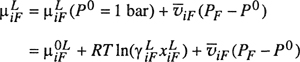
The chemical potential μ_i^M of component i inside the membrane must also be determined at P_F:

(8-124)

Assuming that and taking into account that the equilibrium condition gives the same result as Eq. (8-104) with

In reverse osmosis, the pressure drop from the feed side to the permeate side is located at the phase boundary between the membrane and the liquid permeate. Therefore, equality of the chemical potentials requires

(8-125)

or

(8-126)

where P_P is the pressure in the liquid permeate (usually 1 bar) and subscript P denotes the permeate. Again, assuming that Fick’s law is valid inside the membrane,

(8-127)

If an acceptable approximation for many cases,

Equation (8-128) shows that J_i is enhanced as P_F becomes larger than P_P.

(8-128)

Similar to the other separation processes discussed above, at steady state

(8-129)

Equation (8-129) says that at given composition in the feed mixture, composition in the permeate is obtained by substituting Eq. (8-128) into Eq. (8-129).

Reverse osmosis is applied mostly to dilute aqueous solutions. Therefore, for the solvent water, is a good approximation and Eq. (8-128) can be rewritten as

(8-130)

where Δπ is given by

(8-131)

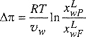
From Eq. (4-42) that gives the osmotic pressure of a dilute solution, we see that Δπ is the difference in osmotic pressure between feed and permeate.

Equation (8-130) tells us that a positive flow J_w is observed when (P_F – P_P) > Δπ; when (P_F – P_P) = Δπ, there is osmotic equilibrium with J_w = 0; when (P_F — P_P) < Δπ, the flux of water is reversed with J_w < 0.

When, in the feed and in the permeate, the mole fraction of solute 2 in the binary aqueous solution << 1, then In (1– ≈ – Substitution into Eq. (8-131) gives

(8-132)

where c₂ ≈ x₂ / is the molar concentration of the solute. Equation (8-132) is another form of the van’t Hoff equation for the osmotic pressure [Eq. (4-44)], valid only for very dilute solutions.

Reverse osmosis is widely used for the separation of water from aqueous ionic solutions, e.g. desalination of seawater. In these applications, it is important that the transport of salt ions through the membrane is as small as possible. For electrically neutral membranes, the transport of ions is determined by their solubility and diffusivity in the membrane. The driving force for ion transport is proportional to the concentration difference of the ions between feed and permeate.

However, when charged membranes or ion-exchange membranes are used instead of neutral membranes, ion transport is also affected by the presence of the charge and number of ionic groups fixed in the membrane. When an ion-exchange membrane is in contact with an ionic solution, ions with charge of the same sign as that of the fixed ionic groups in the membrane are, in principle, excluded and cannot pass through the membrane. This effect is known as Donnan exclusion. Ion-exchange membranes are therefore particularly suitable for separating water from aqueous ionic solutions using reverse osmosis.

Donnan exclusion can be described by equilibrium thermodynamics, as discussed in Sec. 4.11. Let us consider an ion-exchange membrane with fixed negative charges (R^-) and sodium ions Na ⁺ as counterions in contact with a dilute aqueous sodium chloride (NaCl) solution, as shown schematically in Fig. 8-33. Water, Na ⁺ and Cl^- can freely diffuse from the solution into the membrane phase, although Na ⁺ ions can only diffuse in combination with Cl^- ions because electroneutrality must be maintained.

Figure 8-33 Donnan equilibrium when an ionic membrane with fixed negative charges (R^-) is in contact with an aqueous NaCI solution.

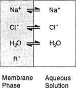
At equilibrium, the chemical potential of sodium chloride is the same in both phases. Assuming ideal solution behavior, i.e. solvent activity (a_s = 1) and the activity of solute i is equal to its molar concentration (a_i = c_i), the equation of phase equilibrium is

(8-133)³⁶

³⁶ Equation (8-133) assumes complete dissociation of sodium chloride, i.e. µ_NaC1 = µ _Na+ + µ_cl^-

Because electroneutrality must be maintained in the membrane phase, and, similarly, because electroneutrality must be maintained in the aqueous solution,

(8-134)

(8-135)

Substitution of Eqs. (8-134) and (8-135) into Eq. (8-133) gives

(8-136)

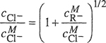
For dilute solutions where Eq. (8-136) reduces to

Equation (8-137) gives the ionic or Donnan equilibrium of anionic solutes in the presence of a charged membrane (or charged macromolecules) with fixed charges R^-. If the concentration in the solution phase is low and the concentration of fixed charges in the membrane is high, Donnan exclusion is very effective. However, with increasing concentration of ions in the solution phase, this exclusion becomes less effective.

(8-137)

The transport equations presented above for pervaporation, gas separation, and reverse osmosis are valid within the frame of the solution-diffusion model in its simplified version, i. e. with constant values of solubility coefficients S_i and neglecting diffusion coupling. An additional problem (not discussed here) is concentration polarization that acts as an additional resistance to the transrnembrane fluxes. Concentration polarization is important mainly in reverse osmosis and in special cases of pervaporation (Heintz and Stephan. 1994; Feng and Huang, 1994; Mulder, 1996; Bhattacharya and Hwang, 1997).

The simplified transport equations allow a qualitative (or semiquantitative) description ³⁷ of the separation characteristics of nonporous membranes. To do so, we need the solubility and the diffusivity of each permeating component in the membrane polymer. Solubilities are obtained from gas, vapor or liquid sorption equilibrium data, and diffusion coefficients from the kinetics of the sorption process (Heintz et al., 1991; Neogi, 1996). At low pressures, gas and vapor sorption (swelling behavior) for amorphous rubbery polymers (polymers above their glass transition temperatures) are modeled successfully with a form of Henry’s law [Eq. (8-108)]. At higher pressures, where sorption behavior deviates from Henry’s law, sorption equilibria can be described, for example, with the Flory-Huggins theory, discussed in Sec. 8.2 (Barbari and Conforti, 1992).

³⁷ For a good quantitative description, the simplifying assumptions have to be removed.

Vapor sorption and the solubilities of liquids and liquid mixtures can be described well with the UNIQUAC model (Sec. 7.7), as reported by Enneking et al. (1993) and Heintz and Stephan (1994). To illustrate, Fig. 8-34 shows a comparison between experimental and calculated solubilities at 333 K for the binary system 2-propartol/water in a thin film of cross-linked poly(vinyl alcohol).³⁸ In Fig. 8-34, the weight fractions of the two components in the polymer are plotted as functions of the weight fraction of the binary mixture outside the membrane. As Fig. 8-34 shows, the solubility curve for 2-propanol has a maximum, indicating a higher solubility for propanol in the mixture than for pure alcohol. Synergistic solubility effects are evident. Nevertheless, both solubility curves predicted from UNIQUAC are in good agreement with experiment. These calculations were made using only binary interaction parameters between the components in the swollen polymer and between the polymer and each of these components. UNIQUAC parameters were obtained from (membrane-free) binary vapor-liquid equilibrium data for 2-propanol/water at 333 K, and from vapor-sorption isotherms for each of the two pure components in the polymer. Similar results have also been reported for the solubility of other aqueous/organic mixtures in poly(vinyl alcohol) and of multicomponent organic mixtures in hydrophobic polymers (Enneking et al, 1993; Enneking et al, 1996).

³⁸ In this cross-linked polymer, about 5% of OH-groups are used for cross-links.

Figure 8-34 Experimental and calculated solubilities for the 2-propanol/water mixture In cross-linked poly(vinyl alcohol) at 333 K. (Heiniz and Stephan, 1994). Calculations based on binary data only.

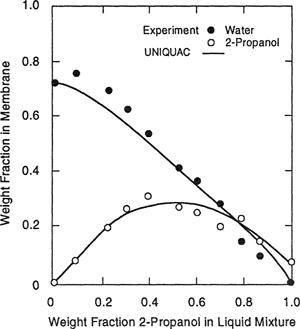
Using solubilities calculated from UNIQUAC, and using the Maxwell-Stefan theory to account for coupling of the diffusion of the two components, Heintz and Stephan (1994) calculated the separation diagram for the mixture 2-propanoI/water with the poly(vinyl alcohol) membrane. Figure 8-35 compares the vapor-liquid equilibrium (VLE) curve at 333 K with the pervaporation curves at permeate pressures of 30 and 130 mbar. This comparison shows that water can be removed with high selectivity at feed weight fractions of 0.8-0.9. Within this composition range, the VLE curve shows the azeotropic point, i.e. pervaporation is effective where distillation is not. As Fig. 8-35 shows, lowering the permeate pressure increases the selectivity for water. The selective poly(vinyl alcohol) top layer of the composite membrane has a thickness of 0.13 µm. Transroembrane fluxes of 0.5-1.0 kg m^-2 h^-1 are obtained at feed weight fractions 0.8-0.9, providing a yield high enough for possible practical application.

Figure 8-35 Separation diagram for the system 2-propanol/water/poly(vinyl alcohol) at 333 K. O, Pervaporation data (Wesslein et al., 1990) at two permeate pressures;—,- - - extended sofution-diffusion (SD) model (Heintz and Stephan, 1994); -.-.- vapor-liquid equilibrium (VLE) for 2-propanol/water.

This section has presented the essential thermodynamics for nonporous-membrane separation processes. Extension of the simple solution-diffusion model presented above can describe more complex cases with coupling effects and concentration polarization.

Membrane-separation processes are sometimes more economical than conventional methods; the equipment is usually less spacious and in some cases membrane processes are “;cleaner” from the environmental point of view. In practical applications, it is sometimes advantageous to use hybrid processes that combine membrane techniques with conventional methods such as distillation (Meckl, 1996; Staudt-Bickel, 1996; Pressly and Ng, 1998). An important task is the synthesis of suitable membranes especially tailored for particular separation problems, having long operation times and high chemical stability in addition to high selectivity and high transmembrane fluxes.

Polymer Gels

Polymer gels are three-dimensional elastic-network materials. In some respects, a gel is similar to a sponge. Brought into contact with a liquid (pure component or solution), a gel may swell or shrink, depending on its initial state and on its interaction with the molecules of the surrounding fluid; if the gel is dry, swelling is likely. Gel swelling depends on the type and concentration of the network-forming polymers (nonionic or ionic homo- and/or copolymers), on the network structure (cross-linking density) and on the composition of the surrounding solution. For ionic systems, swelling also depends on the degree of gel ionization (density of charged groups in the network chains) and on the ionic strength of the surrounding solution.³⁹

³⁹ The ionic strength of an electrolyte solution is defined in Sec. 9.7 by Bq. (9-45).

The heterogeneous system containing a gel consists of three different homogeneous phases:

1. The fluid surrounding the gel.

2. The elastic structure forming the gel.

3. The fluid inside the gel.

The gel-fluid phase is assumed to behave like a bulk fluid phase encaged in an elastic, porous structure, the gel itself. Solvent can pass freely back and forth between the gel-fluid phase and the surrounding solution. However, the porous network structure may allow only selected solute molecules to partition between the two fluid phases, while other solute molecules cannot permeate into the gel (e.g., size exclusion in gel permeation chromatography). A hydrogel is gel that likes water.

Gels may exhibit temperature-induced phase transitions (abrupt changes in volume), as observed for some nonionic hydrogels in aqueous solutions (liavsky et at., 1982; Hirokawa and Tanaka, 1984; Marchetti et al, 1990). Figure 8-36 illustrates a hydrogel undergoing such a phase transition. Nonionic poly(AMsopropylacrylamide) hydrogel coexists with pure water in a swollen state at temperatures below 35 °C, while it collapses at higher temperatures. At about 33°C, there is a phase transition between the shrunken (collapsed) and the swollen state associated with a discontinuous change in volume.

Figure 8-36 Effect of temperature on the volume of a poly(N-isopropylacrylamide) hydrogel in pure water. The expanded graph shows that, when the direction of transition is reversed, some hysteresis may be observed (Hirokawa and Tanaka, 1984).

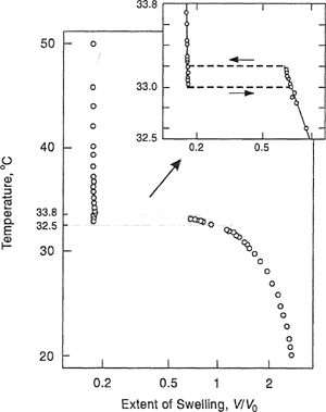
For ionic systems, phase transitions can also be induced by varying the charge density of the gel. If the ionic groups on the polymer correspond to those of a weak acid or base (typically, carboxyl or amino groups), the charge density can be changed by a variation of pH in the surrounding solution (Dušek, 1993).

To illustrate, Fig. 8-37 shows swelling isotherms for four methyl methacrylate (MMA)/dimethyiaminoethyl methacrylate (DMA) copolymers of various comonomer composition as a function of pH at 25°C and a total ionic strength of 0.1 M (Siegel and Firestone, 1988). Whereas MMA is insensitive to pH, the amino group in DMA becomes positively charged when the H⁺ concentration is large (low pH). The data in Fig. 8-37 show that for pH > 6.6, all gels studied here are collapsed, i.e. compact and hydrophobic, regardless of comonomer composition. These collapsed gels contain 10 weight % water or less at swelling equilibrium. Lowering the pH, a critical value of pH is reached where the equilibrium content of water abruptly increases, giving rise to a highly swollen gel. At still lower pH values, the water content continues to increase but at a more gradual rate. The copolymer composition has a strong impact on the equilibrium swelling behavior of the MMA/DMA gels. Changing the MMA/DMA proportion from 70/30 to 86/14 shifts the transition pH from about 6.5 to 4.8, and the water content in the low-pH range changes from about 90 to 40 weight %. The 93/7 mol/mol gel remains compact at all pH; no volume transition occurs.

Figure 8-37 Swelling isotherms for the MMA/DMA copolymers of various cornonomer composition, determined as a function of pH at 25°C and a total ionic strength of 0.1 M. 70/30 mol/mol, º 78/22 mol/mol, 86/14 mol/mol, 93/7 mol/mol (Siegel and Firestone, 1988). MMA = methyl methacrylate (no charge); DMA = dimethylaminoethyl methacrylate (positive charge at low pH).

The abrupt changes ia swelling behavior, induced by changes in external conditions, strongly affect the partitioning of solute species between the gel-fluid phase and the surrounding bulk-fluid phase. Therefore, gels may be suitable for chemical-separation systems (e.g. selective extraction) and as environmentally sensitive barriers for pharmaceutical agents (e.g., physiologically controlled drug delivery devices) (DeRossi et al., 1989; Dušek, 1993; Thiel et al., 1995; Dagani, 1997).

When a gel is in equilibrium with its surroundings, we have not only fluid-phase equilibrium but, in addition, mechanical equilibrium between the elastic, porous network structure, the gel fluid and the surrounding fluid. As the network-forming structure is elastic, its energy depends on its expansion as determined by the volume of the gel-fluid phase. The elastic properties of the network cause the pressure in the gel fluid to be larger than that in the surrounding fluid. This pressure difference may be negligible but for strongly swelling gels it cannot be neglected. In a model describing the phase behavior of polymer gels, therefore, polymer-solution thermodynamics must be combined with the theory of elasticity and, for ionic systems, in addition, with the theory of solutions containing electrolytes. Maurer (1996) gives a comprehensive summary of the fundamental relations that govern not only the phase equilibrium of a gel in contact with a fluid phase but also the equilibrium partitioning of solutes between the gel-fluid phase and the surrounding solution.

For most practical applications, attention has been given to hydrogels, that is, to gels made of hydrophilic polymers. Models for describing aqueous polymer gels may require parameters that are different from those for aqueous polymer solutions (Hirotsu et al., 1987; Inomata et al., 1994) or use too many adjustable parameters (Prange et al, 1989). A simple molecular-thermodynarnic model, developed by Hino (1998), is applicable to polymer solutions as well as to weakly charged polymer gels that can hydrogen bond with the solvent. Hino’s semi-empirical model can be used for predicting the volume-change transition in temperature-sensitive polymer gels, as shown in the following paragraphs.

First we consider a binary polymer solution containing solvent (component 1) and linear polymer (component 2) where solvent molecules are represented by spheres and polymer molecules by freely-jointed chains. We use the extended Flory-Huggins lattice theory discussed in Sec. 8.2 (Qian et al., 1991) to calculate the Helmholtz energy of mixing Δ_mixA:

(8-138)

where k is Boltzmann’s constant, T is the absolute temperature, N_i is the number of molecules of component i, Φ₂ is the volume fraction of the polymer, and g(T, Φ₂) is an empirical function that replaces the customary Flory segmental interaction parameter.

We next consider a polymer gel containing solvent (component 1) and a large cross-linked polymer molecule (component 2) having a small number of ionizable segments. The Helmholtz energy of swelling is given by (Flory, 1953; Tanaka, 1980)

(8-139)⁴⁰

⁴⁰ Equation (8-139) assumes that the three contributions are essentially independent of each other. This equation is often referred to as the FSory-Rehner theory.

(8-139)

where Δ_mixA, ΔA^elas and ΔA^ion represent mixing, elastic, and electrostatic contributions, respectively.

Provided that cross-linking in the gel is modest (i.e. long strands of polymer between cross-link points), the mixing contribution is (Flory, 1953)

(8-140)

For the Helmholtz energy change due to elastic deformation, Hino uses an expression given by Birshtein and Pryamitsyn (1991) and Grosberg and Kuznetsov (1992):

(8-141)

where α is the expansion factor and v is the total number of chains. The expansion factor is given by (Flory, 1976, 1977; Erman and Flory, 1986; Painter and Shenoy, 1993):

(8-142)

where Φ₀ is the volume fraction of polymer in the reference state where the conformation of network chains is closest to that of unperturbed Gaussian chains (Khokhlov, 1980); Φ₀ is usually approximated by the volume fraction of polymer at preparation of the gel.

Finally, for a small charge density, Hino expresses the electrostatic effect using the van’t Hoff equation (Ricka and Tanaka, 1984; Otake et al, 1989):

(8-143)

where m is the number of charged segments per network chain between points of cross-linking, and r_n is the number of segments per network chain.

For phase-equilibrium calculations, we introduce the Flory χ parameter, defined by the product of two empirical functions (Qian et al., 1991; Bae et al., 1993):

(8-144)

where B(Φ) is a function of composition and D(T) is a function of temperature.

We also define reduced temperature and interchange energy ε by

(8-145)

(8-146)

where ε_ij (i, j = 1, 2) is the segmental interaction energy for non-specific interactions between components i and j.

For B(Φ), we use an expression from Bae et al. (1993). For D(T), we use an expression based on the work of ten Brinke and Karasz (1984) and Hino et al. (1993, 1993a):

(8-147)

(8-148)

where z is the lattice coordination number (z = 6 in this work), δε₁₂ is the difference between the segmental interaction energy for specific interactions and that for non-specific interactions, s_l2 is the ratio of degeneracy of non-specific interactions to that of specific interactions, and b is an empirical parameter, all obtained from independent polymer-solution data. Equation (8-147) accounts for specific interactions between unlike molecules. As already discussed in Sec. 8.2, with this expression it is possible to predict lower-criticai-solution temperature (LCST) behavior due to specific interactions such as hydrogen bonding.

At equilibrium, μ₁ (surrounding pure solvent) is equal to μ₁ (in the gel). The chemical potential of the solvent in the gel is found from differentiation of ΔA^swe with respect to N₁. We then have

(8-149)

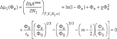
where Δμ₁ is the change in chemical potential of solvent upon mixing, and V is the volume of the gel. For the elastic term in Eq. (8-149), we use Eq. (8-141). For the mixing term, we use the extended Flory-Huggins theory presented above.

Under the specific conditions where two gel phases can coexist at one temperature, a polymer gel exhibits a discontinuous volume change. The conditions for coexistence of the two gel phases are (Marchetti et al., 1990)

(8-150)

and

(8-151)

where superscripts ’and” denote coexisting phases, i.e. the expanded and the collapsed gel. From the Gibbs-Duhem equation, Eq. (8-151) can be replaced by

(8-152)

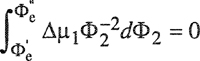
Hino (1998) applied his model to poly(N-isopropylacrylamide) (PNIPAAm) gels in water and to aqueous solutions of non-crosslinked PNIPAAm. The polymer solutions exhibit LCST behavior at about 32°C and from these data the following parameters were obtained: ε = 2.92 kJ mol^-1, δε₁₂/ε=-7, and b = 0.65, with s₁₂ preset to 5000 as discussed in Sec. 8.2. Using the same parameters for the mixing term, Hino’s model can also represent the phase diagram of neutral PNIPAAm gels. As shown in Fig. 8-36, these gels exhibit abrupt volume contractions at about 32.5-33.8°C. Figure 8-38 illustrates that the temperature of this volume transition is represented quantitatively with m = 0 (nonionic gel) and with r_n = 89 in Eq. (8-149) adjusted such that the swelling ratio is 2.5 at 20°C with Φ₀ = 0.07, as indicated by the PNIPAAm gels studied by Hirotsu et al. (1987).

Figure 8-38 Swelling-ratio curve for neutral PNIPAAm gel in water calculated with the model of Hino (1998). Experimental transition temperature range is 32.5-33.8°C (Hirotsu et al., 1987).

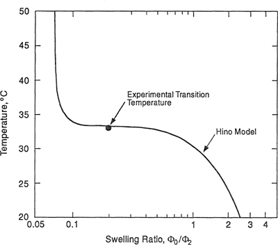
PNIPAAm gels copolymerized with ionizable monomers swell more than aeuttal PNIPAAm gels (Beltran et al, 1990) and exhibit more abrupt volume contractions (Hirotsu et al., 1987; Hino et al., 1993). That observation is predicted by Hino’s model with m > 0, i.e. for gels with ionizable segments in the network-forming polymer chains.

The experimental phase behavior of neutral and ionic gels has been studied extensively. Applications of gels in chemical engineering, medicine, and biotechnology are, as yet, in an early stage (Dagani, 1997).

8.5 Summary

There has been much progress in the thermodynamics of polymer solutions since the initial path-breaking work of Flory and Huggins, more than 50 years ago. That initial work was closely tied to the filled-lattice concept that limited consideration to those mixtures where there is no volume change upon mixing at constant temperature and pressure. To relieve that severe limitation, much attention has been given toward developing an equation of state suitable for polymers, polymer/solvent mixtures and polymer blends.

While the limitation of the constant-volume assumption of filled-lattice thermodynamics was recognized early, a major stimulus to develop an equation of state for polymer-solvent systems was provided over 30 years ago when experimental results indicated the common existence of a lower critical-solution temperature that lies above the upper critical-solution temperature. Classical lattice thermodynamics cannot explain such phase behavior. A first necessary test for any proposed equation of state for mixtures is that it must be able to reproduce phase behavior that includes both lower and upper critical-solution temperatures where the lower critical-solution temperature is larger than the upper critical-solution temperature. All proposed equations of state discussed here can meet that test, at least in principle.

Upon introducing specific attraction between unlike components (e.g. hydrogen bonding), filled-lattice theory can be modified to give a lower critical-solution temperature that lies below the upper critical-solution temperature. Such modification can also be applied to an equation of state with the same result.

As discussed in this chapter, for fluids containing chain molecules, equations of state can be derived along several lines: lattice-fluid or hole theories, where a lattice contains occupied and unoccupied lattice sites (holes); and free-standing theories, independent of any geometric construct such as cells or lattices, where the volumetric properties of an assembly of chains are described by a statistical mechanical method (the integral theory of fluids) not discussed here. Analytical results can be obtained from the integral theory of fluids for hard non-attracting chains. For attractive chains, it is necessary to use numerical methods or else to introduce attractive forces as a perturbation about results for non-attractive chains.

All these theories can successfully describe the P-V-T properties of pure liquid polymers using (typically) three or four adjustable molecular parameters that, respectively, reflect chain length, segment size, potential energy between two nonbonded segments and (sometimes) chain flexibility or “floppiness” as a measure of external degrees of freedom.

Regrettably, extension to mixtures shows serious deficiencies in all of these theories. First, these theories fail to account for long-range correlation; when one segment of a chain moves, that movement influences the movement of other segments in the same chain. Second, these theories are for simple chains and therefore do not account for the effect of chain branching or of rings within a chain. Third, and perhaps most serious, all of these theories are of the mean-field type that fail to account for the contribution of fluctuations in density and composition. It has been known for many years that the mean-field approximation is valid only at high densities and high temperatures. Therefore, when the theories described here are used in the critical region (where fluctuations are large), poor results are often obtained; if model parameters are fixed using critical data (coordinates of upper or lower critical-solution temperatures), the calculated two-liquid region is too narrow; but if parameters are fixed from LLE data remote from critical, erroneous predictions are obtained for critical temperatures and compositions.

For polymer/solvent mixtures, reliable VLE can be calculated easily (except when the solvent is near its critical temperature) because such calculation requires only the chemical potential of the solvent; the chemical potential of the polymer does not enter the calculation because polymers are nonvolatile. However, VLE calculation may depend on the range of composition considered; binary parameters obtained from dilute polymer-solution VLE are often different from those obtained from concentrated polymer-solution VLE.

Accurate calculation of LLE is much more difficult for polymer/solvent mixtures because typically, the polymer is dilute in one liquid phase and concentrated in the other liquid phase. Mean-field approximations are not good for a dilute phase. If binary parameters are found for a solution dilute in polymer, they are likely to be different from those found for a solution where the polymer concentration is large. Mean-field approximations introduced in most equations of state are not valid for dilute solutions. Distinguishing between intramolecular and intermolecular segment-segment interactions is not as important in concentrated solutions as it is in dilute solutions. Further, unlike VLE, LLE are often sensitive to the polymer’s polydispersity.

It is likely that several reasons may be responsible for the failure of EOS theories to represent liquid-liquid equilibrium with good accuracy. One reason may follow from the conventional procedure for finding EOS constants for the pure polymer. That procedure is based on reduction of P-V-T data for pure liquid polymers; the characteristic energy parameter obtained from perturbed hard-sphere-chain equations is often too large, perhaps because pure liquid polymers have chains with extensive entanglement. The characteristic energy parameter, therefore, includes the energy of disentanglement. However, the calculated free energy of mixing of a polymer with a solvent makes no provision for disentangling the pure polymer prior to dissolution. Better results for liquid-liquid equilibrium may perhaps, be obtained if the mixture calculations include a contribution that reflects the disentanglement of polymer chains upon mixing. That contribution may be important for polymer-solvent mixtures but probably tends to cancel for polymer-polymer blends.

These problems are not readily observed from model calculations but they become clear when calculated results are compared with experiment. Errors introduced by mean-field approximations are evident when the top of the liquid-liquid coexistence curve is insufficiently flat and whenever calculations of phase equilibria are compared with experiment over a large range of polymer concentration, from very dilute to appreciable polymer concentration. Given a set of molecular parameters, it is possible to fit experimental data for one equilibrium liquid phase but, to fit the other equilibrium liquid phase, a different set of molecular parameters is often required. These problems are much reduced when equations of state are used for polymer blends. For mixtures of polymers, good results can often be obtained because errors introduced by mean-field approximations tend to cancel.

In general, two conceptually different mean-field approximations are invoked during the development of equations of state for chain molecules, regardless of their framework. To calculate the entropy of a collection of polymer molecules, even in the absence of attractive forces, the number of available configurations must be properly calculated without neglect of correlations between segments of a chain that are not nearest neighbors along the chain. This neglect is the essence of the first mean-field approximation. A second mean-field approximation is associated with calculating the potential energy; in that approximation, chain connectivity and the correlation between segments are improperly ignored.

The inadequacy of mean-field approximations was recognized many years ago; it is indicated in the classic text by Flory published in 1953. At present we do not have a useful analytical equation of state for mixtures that overcomes this inadequacy. An alternative to an analytical equation is provided by molecular simulation calculations but these are not as yet practical for routine engineering applications. The current literature has reported several simulation calculations for non-attractive mixtures of chains; only very recently have such calculations been made for pure-polymer liquids with attractive forces. It is likely that we will soon see simulation calculations also for mixtures of attractive chains and solvents. Such simulations are likely to provide better agreement with experiment over the entire composition range. As computers become more powerful and as more efficient computing strategies become available, simulation calculations may eventually replace analytical equations of state. However, for the near future, analytical equations of state will remain useful for application provided that their use is restricted to narrow ranges of composition or else, provided that they are modified semi-empirically to overcome limitations imposed by the mean-field approximation.

Finally, there is a geometric consideration that is usually overlooked. In a polymer chain, the distance between bonded segments is probably somewhat smaller than the collision diameter that characterizes the interaction between non-bonded segments. Therefore, the parameter σ used in the reference part of the EOS (i.e. the part for non-attracting chains) is not the same as that used in the perturbation part of the EOS (i.e. the part that corrects for attractive forces). To refrain from using an excessive number of parameters, it is customary to ignore this difference in the two characteristic length parameters. That procedure does not affect the ability of an EOS to fit pure-polymer data but it may have a significant effect on liquid-liquid equilibria for polymer/solvent systems.

While polymers have a multitude of applications in chemical technology, thin films of polymers (nonporous membranes) are particularly useful for separation operations. Design of such operations requires transport properties (diffusivities) in addition to thermodynamic properties.

When a model for polymer solutions is combined with a model for polymer network elasticity, it is possible to construct a theory for the properties of a polymer gel in contact with a swelling solvent. That theory shows the possibility of a first-order ohase transition in response to a change in temperature. If the polymer gel contains groups that are weakly acid (or basic), a similar phase transition can respond to a change in pH of the solvent. As a result, polymer gels have potential as “smart” materials that can exhibit a strong response to a small change of environment. Thanks to thermodynamic analysis, we now have a good understanding of the fundamental properties of gel-solvent systems but many important details must be clarified before this understanding becomes truly quantitative.

References

Amjad, Z., (Ed.), 1993, Reverse Osmosis: Membrane Technology, Water Chemistry, and Industrial Applications. New York: Van Nostrand Reinhold.

Bae, Y. C, J. J. Shim, D. S. Soane, and J. M. Prausnitz, 1993, J. Appl. Polym. Sci, 47: 1193.

Banaszak, M., C. K. Chen, and M. Radosz, 1996, Macromolecules, 29: 6481.

Barbari, T. A. and R. M. Conforti, 1992, J. Polym. Sci., PartB: Polym. Phys., 30: 1261.

Barton, A. F. M., 1990, Handbook of Solubility Parameters. Boca Raton; CRC Press.

Baudot, A. and M. Matin, 1997, Trans. I. Chem. Eng., 75: 117.

Bawendi, M. G., K. F. Freed, and U. Mohanty, 1987, J. Chem. Phys., 87: 5534.

Bawendi, M. G. and K. F. Freed, 1988, J. Chem. Phys., 88: 2741.

Beltran, S., H. H. Hooper, H. W. Blanch, and J. M. Prausnitz, 1990, J. Chem. Phys., 92: 2061.

Berens, A. R., G. S. Huvard, R. W. Korsmeyer, and F. W. Kunig, 1992, J. Appl. Polym. Sci., 46: 231.

Bhattacharya, S. and S.-T. Hwang, 1997, J. Membrane Sci., 132: 73.

Birshtein, T. M. and V. A. Pryamitsyn, 1991, Macromolecules, 24: 1554.

Blanks, R. F. and J. M. Prausnitz, 1964, Ind. Eng. Chem. Fundam., 3: 1.

Böddeker, K.-W. and G. Bengtson, 1991, Selective Pervaporation of Organics from Water. In Pervaporation Membrane Separation Processes, (R. Y. M. Huang, Ed.). Amsterdam: Elsevier.

Bondi, A., 1968, Physical Properties of Molecular Crystals, Liquids and Glasses. New York: John Wiley & Sons.

Bonner, D. C., A. Bellemans, and J. M. Prausnitz, 1972, J. Polym. Sci, Part C, 39: 1.

Burrell, H., 1955, Interchem. Rev., 14: 3, 31.

Chapman, W. G., K. E. Gubbins, G. Jackson, and M. Radosz, 1990, Ind. Eng. Ghent. Res., 29: 1709.

Chen, S.-J. and M. Radosz, 1992, Macromolecules, 25: 3089.

Chen, S.-J., I. G. Economou, and M. Radosz, 1992, Macromolecules, 25: 4987.

Chen, S.-J., I. G. Economou, and M. Radosz, 1993, Fluid Phase Equilibria, 83: 391.

Chen, S.-J., Y. C. Chiew, J. A. Gardecki, S. Nilsen, and M. Radosz, 1994, J. Polym. Sci, Part B: Polym. Phys., 32: 1791.

Chen, S.-J., M. Banaszak, and M. Radosz, 1995, Macromolecules, 28: 1812.

Chiou, J. S., J. W. Barlow, and D. R. Paul, 1985, J. Appl. Polym. Sci, 30: 2633.

Condo, P. D. and K. P. Johnston, 1992, Macromolecules, 25: 6730.

Condo, P. D., I. C. Sanchez, C. G. Panayiotou, and K. P. Johnston, 1992, Macromolecules, 25: 6119.

Condo, P. D. and M. Radosz, 1996, Fluid Phase Equilibria, 117: 1.

Costas, M. and B. C. Sanctuary, 1981, J. Phys. Chem., 85: 3153.

Costas, M. and B. C. Sanctuary, 1984, Fluid Phase Equilibria, 18: 47.

Cotton, N. J., K. D. Bartle, A. A. Clifford, and C. J. Dowle, 1993, J. Appl. Polym. Sci, 48: 1607.

Cowie, J. M., 1991, Polymers: Chemistry and Physics of Modern Materials, 2^nd Ed. London: Chapman &Hall.

Dagani, R., 1997, Chem. Eng. News, 75: 26.

Daneshvar, M., S. Kim, and E. Gulari, 1990, J. Phys. Chem., 94: 2124.

DeRossi, D., K. Kajiwara, Y. Osada, and A. Yamauchi, 1991, Polymer Gels: Fundamentals and Biomedical Applications. New York: Plenum Press.

Di Marzio, E. A. and J. H. Gibbs, 1963, J. Polym. Sci, Part A, 1: 1417.

Dickman, R. and C. K. Hall, 1986, J. Chem. Phys., 85: 4108.

Donohue, M. D. and J. M. Prausnitz, 1975, Can. J. Chem., 53: 1586.

Dudowicz, J. and K. F. Freed, 1991, Macromolecules, 24: 5112.

Dušek, K., (Ed.), 1993, Responsive Gels: Volume Transitions I and Volume Transitions II, Advances in Polymer Science, Vols. 109 and 110. Heidelberg: Springer.

Eichinger, B. E. and P. J. Flory, 1968, Trans. Faraday Soc., 64: 2053.

Eichinger, B. E. and P. J. Flory, 1968a, Trans. Faraday Soc., 64: 2035.

Enneking, L., W. Stephan, and A. Heintz, 1993, Ber. Bunsenges. Phys. Chem., 97: 912.

Enneking, L., A. Heintz, and R. N. Lichtenthaler, 1996, J. Membrane Sci, 115: 561.

Erman, B. and P. J. Flory, 1986, Macromolecules, 19: 2342.

Fast, J. D., 1962, Entropy, Philips Technical Library. Eindhoven: Centrex Publishing.

Feng, X. and R. Y. M. Huang, 1994, J. Membrane Sci, 92: 201.

Feng, X. and R. Y. M. Huang, 1997, Ind. Eng. Chem. Res., 36: 1048.

Flory, P. J., 1941, J. Chem. Phys., 9: 660.

Flory, P. J., 1942, J. Chem. Phys., 10: 51.

Flory, P. J., 1953, Principles of Polymer Chemistry. Ithaca: Cornell University Press.

Flory, P. J., R. A. Orwoll, and A. Vrij, 1964, J. Am. Chem. Soc., 86: 3507, 3515.

Flory, P. J., 1965, J. Am. Chem. Soc., 87: 1833.

Flory, P. J. and R. A. Orwoll, 1967, J. Am. Chem. Soc., 89: 6814, 6822.

Flory, P. J., J. L. Ellenson, and B. E. Eichiager, 1968, Macromolecules, 1: 279.

Flory, P. J., 1970, Discuss. Faraday Soc., 49: 7.

Flory, P. J., 1976, Proc. Roy. Soc. London, Ser. A., 351: 351.

Flory, P. J., 1977, J. Chem. Phys., 66: 5720.

Freed, K. F., 1985, J. Phys. A: Math. Gen., 18: 871.

Gibbs, J. H. and E. A. Di Marzio, 1958, J. Chem. Phys., 28: 373.

Gregg, C. J., S.-J. Chen, F. P. Stein, and M. Radosz, 1993, Fluid Phase Equilibria, 83: 375.

Grosberg, A. Y. and D. V. Kuzmtsov, 1992, Macromolecules, 25: 1970.

Grulke, E. A., 1989, Solubility Parameter Values. In Polymer Handbook, 3^rd Ed., (J. Brandrup and E. H. Immergut, Eds.). New York: John Wiley & Sons.

Guggenheim, E. A., 1944, Proc. Roy. Soc. A, 183: 203.

Guggenheim, E. A., 1952, Mixtures. Oxford: Clarendon Press.

Gupta, R. B. and J. M. Prausnitz, 1995, J. Chem. Eng. Data, 40: 784.

Gupta, R. B. and J. M. Prausnitz, 1996, Ind. Eng. Chem. Res., 35: 1225.

Hansen, C. M., 1967, J. Paint Technol, 39:104, 505.

Hansen, C. M. and K. Skaarup, 1967a, J. Paint Technol., 39: 511.

Hansen, C. M. and A. Beerbower, 1971, Solubility Parameters. In Encyclopedia of Chemical Technology (Kirk-Othmer), 2^nd Ed., Suppl. Vol. (H. F. Mark, J. J. McKetta, and D. F. Othmer, Eds.). New York: Wiley-Interscience.

Harismiadis, V. I, G. M. Kontogeorgis, Aa. Fredenslund, and D. P. Tassios, 1994, Fluid Phase Equilibria, 96: 93.

Heintz, A. and R. N. Lichtenthaler, 1977, Ber. Bunsenges. Phys. Chem., 81: 921.

Heintz, A. and R, N. Lichtenthaler, 1980, Ber. Bunsenges. Phys. Chem.., 84: 727.

Heintz, A., H. Funke, and R. N. Lichtenthaler, 1991, Sorption and Diffusion in Pervaporation Membranes. In Pervaporation Membrane Separation Processes, (R. Y. M. Huang, Ed.). Amsterdam: Elsevier.

Heintz, A. and W. Stephan, 1994, J. Membrane Sci, 89: 143,153.

Henderson, D., 1974, Ann. Rev. Phys. Chem., 25: 461.

Hildebrand, J. H., 1947, J. Chem. Phys., 15: 225.

Hino, T., S. M. Lambert, D. S, Soaae, and J. M. Prausnitz, 1993, AIChE J., 39: 837.

Hino, T., S. M. Lambert, D. S. Soane, and J. M. Prausnitz, 1993a, Polymer, 34: 4756.

Hino, T., Y. Song, and J. M. Prausaitz, 1994, Macromolecules, 27: 5681.

Hino, T., Y. Song, and J. M. Prausnitz, 1995, Macromolecules, 28: 5709,5717, 5725.

Hino.T. and J. M. Prausnitz, 1998, Polymer, 39: 3279.

Hirokawa, Y. and T. Tanaka, 1984, J. Chem. Phys., 81: 6379.

Hirotsu, S., Y. Hirokawa and T. Tanaka, 1987, J. Chem. Phys., 87: 1392.

Hirschfelder, J., D. Stevenson, and H. Eyring, 1937, J. Chem. Phys., 5: 896.

Honnell, K. G. and C. K. Hall, 1989, J. Chem. Phys., 90: 1841.

Hu, Y., S. M. Lambert, D. S. Soane, and J. M. Prausnitz, 1991, Macromolecules, 24: 4356.

Huang, R. Y. M., (Ed.), 1991, Pervaporation Membrane Separation Processes. Amsterdam: Elsevier.

Huggins, M. L., 1941, J. Phys. Chem., 9: 440.

Huggins, M. L., 1942, Ann. N. Y. Acad. Sci., 43: 1.

Ilavsky, M., J. Hrouz and K. Ulbrich, 1982, Polym. Bull, 7: 107.

Inomata, H., K. Nagahama and S. Saito, 1994, Macromolecules, 27: 6459.

Inui, K., H. Okumura, T. Miyata, and T. Uragami, 1997, J. Membrane Sci., 132: 193.

Iwai, Y. and Y. Arai, 1991, J Japan Petrol. Inst., 34: 416.

Kalospiros, N. S. and M. E. Paulaitis, 1994, Chem. Eng. Sci., 49: 659.

Kammer, H.-W., T. Inoue, and T. Ouginawa, 1989, Polymer, 30: 888.

Kaul, B. K., M. D. Donohue, and J. M. Prausnitz, 1980, Fluid Phase Equilibria, 4: 171.

Khokhlov, A. R., 1980, Polymer, 21: 376.

Kim, C. K. and D. R. Paul, 1992, Polymer, 33: 1630, 2089, 4941.

Kleintjens, L. A. and R. Koningsveld, 1980, Colloid Polym. Sci., 258: 711.

Kleintjens, L. A. and R. Koningsveld, 1982, Sep. Sci. Tech., 17: 215.

Koningsveld, R. and A. J. Staverman, 1968, J. Polym. Sci. Part A-2, 6: 305, 325, 349.

Koningsveld, R., L. A. Kleintjens, and A. R. Shultz, 1970, J. Polym. Sci. Part A-2, 8: 1261.

Koningsveld, R. and L. A. Kleintjens, 1971, Macromolecules, 4: 637.

Kontogeorgis, G. M., V. I. Harismiadis, Aa. Fredenslund, and D. P. Tassios, 1994, Fluid Phase Equilibria, 96: 65.

Lambert, S. M., D. Soane, and J. M. Prausnitz, 1993, Fluid Phase Equilibria, 83: 59.

Lambert, S. M., Y. Song, and J. M. Prausnitz, 1995, Macromolecules, 28: 4866.

Lambert, S. M., Y. Song, and J. M. Prausnitz, 1998, Equations of State for Polymer Systems. In Equations of State for Fluids and Fluid Mixtures (J. V. Sengers, M. B. Ewing, R. F. Kayser, C. J. Peters, and H. J. White, Jr., Eds.). Oxford: Blackwell Scientific.

Lichtenthaler, R. N., D. S. Abrams, and J. M. Prausnitz, 1973, Can. J. Chem., 51: 3071.

Lichtenthaler, R. N., D. D. Liu, and J. M. Prausnitz, 1974, Ber. Bunsenges. Phys. Chem., 78: 470.

Lichtenthaler, R. N., D. D. Liu, and J. M. Prausnitz, 1978, Macromolecules, 11: 192.

Madden, W. G., A. I. Pesci, and K. F. Freed, 1990, Macromolecules, 23: 1181.

Madden, W. G., J. Dudowicz, and K. F. Freed, 1990a, Macromolecules, 23: 4803.

Marchetti, M., S. Prager, and E. L. Cussler, 1990, Macromolecules, 25: 1760, 3445.

Maurer G. and J. M. Prausnitz, S996, Fluid Phase Equilibria, 115:113.

McMaster, L. P., 1973, Macromolecules, 6: 760.

Meckl, K. and R. N. Lichtenthaler, 1996, J. Membrane Sci., 113:81.

Mulder, M., 1996, Basic Principles of Membrane Technology, 2^nd Ed. Dordrecht: Kluwer Academic Publishers.

Myrat, C. D. and J. S. Rowlinson, 1965, Polymer, 6: 645.

Neogi, P., (Ed.), 1996, Diffusion in Polymers. New York: Marcel Dekker.

Nguyen, Q. T., C. Léger, P. Billard, and P. Lochon, 1997, Polymers Adv. Techn., 8: 487.

Noble, R. D. and S. A. Stern, (Eds.), 1995, Membrane Separation Technology: Principles and Applications, Membrane Science and Technology, Vol. 2. Amsterdam: Elsevier.

Ohzono, M., Y. Iwai, and Y. Arai, 1984, J Chem. Eng. Japan, 17: 550.

Orwoll, R. J., 1977, Rubber Chem. Technol., 50: 452.

Otake, K., H. Inomata, M. Konno, and S. Saito, 1989, J. Chem. Phys., 91: 1345.

Painter, P. C. and S. L. Shenoy, 1993, J. Chem. Phys., 99: 1409.

Panayiotou, C. and J. H. Vera, 1981, Can. J. Chem. Eng., 59: 501.

Panayiotou, C. and J. H. Vera, 1982, Polym. J., 14: 681.

Panayiotou, C., 1987, Macromolecules, 20: 861.

Panayiotou, C. and I. C. Sanchez, 1991, Macromolecules, 24: 6231.

Park, D.-W. and R.-J. Roe, 1991, Macromolecules, 24: 5324.

Patterson, D., 1969, Macromolecules, 2: 672.

Patterson, D. and G. Delmas, 1970, Discuss. Faraday Soc., 49: 98.

Pope, D. S., I. C. Sanchez, W. J. Koros, and G. K. Fleming, 1991, Macromolecules, 24: 1779.

Pouchly, J. and D. Patterson, 1976, Macromolecules, 9: 574.

Prange, M. M., H. H. Hooper and J. M. Prausnitz, 1989, AIChE J., 35: 803.

Pressly, T. G. and K. M. Ng, 1998, AIChE J., 44: 93.

Prigogine, I., 1957, The Molecular Theory of Solutions. Amsterdam: North-Holland.

Qian, C., S. J. Mumby, and B. E. Eichinger, 1991, J. Polym. Sci, Part B: Polymer Physics, 29: 635.

Qian, C., S. J. Mumby, and B. E. Eichinger, 1991a, Macromolecules, 24: 1655.

Rave, A., 1995, Principles of Polymer Chemistry. New York: Plenum Press.

Ricka, J. and T. Tanaka, 1984, Macromolecules, 17: 2916.

Rodgers, P. A. and I. C. Sanchez, 1993, J. Polym. Sci Part B: Polym. Phys., 31: 273.

Roe, R.-J. and W.-C. Zin, 1980, Macromolecules, 13: 1221.

Rostami, S and D. J. Walsh, 1985, Macromolecules, 18: 1228.

Sanchez, I. C. and R. H. Lacombe, 1976, J. Phys. Chem., 80: 2352, 2568.

Sanchez, I. C. and R. H. Lacombe, 1977, J. Polym. Sci, Polym. Lett. Ed., 15: 71.

Sanchez, I. C. and R. H. Lacombe, 1978, Macromolecules, 11:1145.

Sanchez, I. C., 1987, Encyclopedia of Physical Science and Technology, Vol. XL New York: Academic Press.

Sanchez, I. C. and A. C. Balazs, 1989, Macromolecules, 22: 2325.

Sanchez, I. C. and P. A. Rodgers, 1990, Pure & Appl. Chem., 62: 2107.

Sanchez, I. C. and C. Panayiotou, 1994, Equation of State Thermodynamics of Polymer and Related Solutions. In Models for Thermodynamic and Phase Equilibria Calculations, (S. I. Sandler, Ed.). New York: Marcel Dekker.

Scott, R. L. and P. H. van Konynenburg, 1970, Discuss. Faraday Soc., 49: 87.

Siegel, R. A. and B. A. Firestone, 1988, Macromolecules, 21: 3254.

Simha, R. and T. Somcynsky, 1969, Macromolecules, 2: 342.

Siow, K. S., G. Delmas, and D. Patterson, 1972, Macromolecules, 5: 29.

Smith, S. W., C. K. Hall, and B. D. Freeman, 1995, Phys. Rev. Lett., 75: 1316.

Somcynsky, T. and R. Simha, 1971, J. Appl. Phys., 42: 4545.

Song, Y., S. M. Lambert, and J. M. Prausnitz, 1994, Ind. Eng. Chem. Res., 33: 1047.

Song, Y., S. M. Lambert, and J. M. Prausnitz, 1994a, Chem. Eng. Sci, 49: 2765.

Staudt-Bickel, C. and R. N. Lichtenthaler, 1996, J. Membrane Sci., 111: 135.

Staverman, A. J., 1950, Recl. Trav. Chim. Pays-Bas, 69: 163.

Streicher, C., L. Asselineau, and A. Forestière, 1995, Pure & Appl. Chem., 67: 985.

Swinton, F. L., 1976, Ann. Rev. Phys. Chem., 27: 153.

Tanaka, T., 1980, Phys. Rev. Lett., 45: 1636.

ten Brinke, G. and F. E. Karasz, 1984, Macromolecules, 17: 815.

Thiel, J., G. Maurer, and J. M. Prausnitz, 1995, Chem.-lng.-Tech., 67: 1567.

Tompa, H., 1952, Trans. Farad. Soc., 48: 363.

Wesslein, M., A. Heintz, and R. N. Lichtenthaler, 1990, J. Membrane Set., 51: 169.

Wijmans, J. G. and R. W. Baker, 1995, J. Membrane Sci, 107: 1.

Wissinger, R. G. and M. E. Paulaitis, 1991, Ind. Eng. Chem. Res., 30: 842.

Wissinger, R. G. and M. E. Paulaitis, 199la, J. Polym. Sci., Part B: Polym. Phys., 29: 631.

Wu, C.-S. and Y.-P. Chen, 1994, Fluid Phase Equilibria, 100: 103.

Yoshikawa, M., S. Takeuchi, and T. Kitao, 1997, Angew. Makromol. Chem., 245: 193.

Young, R. J. and P. A. Lovell, 1991, Introduction to Polymers, 2^nd Ed. London: Chapman & Hall.

Zeman, L. and D. Patterson, 1972, J. Phys. Chem., 76: 1214.

Problems

1. In polymer solutions, it is convenient to define an activity coefficient Γ₁ = a₁/Φ₁, where a is the activity, Φ is the volume fraction, and subscript 1 refers to the volatile component. When Φ₁ is very small, ; the Flory-Huggins equation gives

where χ is the Flory interaction parameter and r = υ₂/υ₁; υ₂ is the molar volume of the polymer and υ₁ is that of the solvent. For high-molecular-weight polymers, r >> 1.

A film of poly(vinyl acetate) contains traces of isopropyl alcohol. For health reasons, the alcohol content of the film must be reduced to a very low value; government regulations require that Φ₁ < 10^-4. To remove the alcohol, it is proposed to evaporate it at 125°C. At this temperature, chromatographic experiments give χ = 0.44 and the vapor pressure of isopropyl alcohol is 4.49 bar. Calculate the low pressure that must be maintained in the evaporator to achieve the required purity of the film. Under the conditions prevailing here, the activity is given by the ratio of partial pressure to vapor pressure. The polymer is involatile.

2. Estimate the total pressure of a liquid solution containing 50 wt% poly(vinyl acetate) and 50 wt% vinyl acetate at 125°C.

Data (all at 125°C) are as follows:

The molecular weight of the polymer is 8.34x10⁴. From chromatographic measurements at 125°C, Henry’s constant (partial pressure/weight fraction) for vinyl acetate in poly(vinyl acetate) is 18.3 bar. In your calculation, what is the most important simplifying assumption?

3. (a) Derive Flory equation of state [Eq. (8-45)] from the generalized van der Waals partition function given by Eq. (8-39).

(b) Derive Sanchez-Lacombe equation of state [Eq. (8-84)] from the configurational partition function given by Eq. (8-82).

4. In a binary system solvent (l)/polymer (2), the composition at which the UCST occurs depends on polymer molecular weight (see Fig. 8-8). According to the Flory-Huggins theory, the critical segment fraction is Derive this expression.

5. The characteristic parameters of Flory equation of state for hexamethyl disiloxane (HMDS) and poly(dimethyl slloxanes) (PDMS) of various molecular weights are listed in Table 8-5. For mixtures of HMDS (1)/PDMS (2), Flory parameter χ = 0 is a good approximation. Calculate In γ₁ for the various binary mixtures at and discuss the dependence on molecular weight.

6. The solubility coefficient (S) and diffusion coefficient (D) of oxygen and nitrogen in silicone rubber at 20°C are:

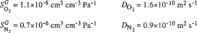
Calculate the separation factor and the fluxes of oxygen and nitrogen through a 5 μm thick membrane of silicone rubber with air at 2 bar as feed and vacuum on the permeate side.

7. A polymeric membrane, mechanically supported by a metal screen, is used to separate a gaseous mixture of carbon dioxide (1) and methane (2) at 300 K, as illustrated below.

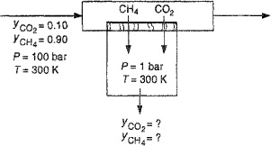
On the upstream side, in contact with the membrane, is a gaseous mixture at 100 bar containing 10 mol % carbon dioxide and 90 mol % methane. The fluxes of carbon dioxide and methane through the membrane follow Pick’s law. Diffusion coefficients (cm² s^-1) are 5x10^-6 for carbon dioxide and 50x10^-6 for methane. The membrane’s thickness is 1 mm. Downstream preessure is 1 bar. Calculate the composition of the gas downstream from the membrane.

Second virial coefficients (cm³ mol^-1) at 300 K: B₁₁ = -121; B₁₂ = -55; B₂₂ = -41.

At 1 bar and 300 K, the partial molar volumes at infinite dilution and Henry’s constants (based on the molar concentration) of component i dissolved in the polymeric membrane are:

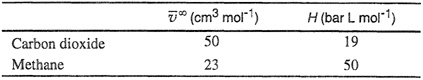
8. Consider a reverse-osmosis process for producing fresh water from seawater at 25°C. Assume that a perfectly selective membrane is available, i.e., the membrane passes water but no salts.

(a) To achieve a water flux of 7.2x10^-4 g cm^-2 s^-1, what upstream pressure must be used to operate this process?

(b) How many square feet of membrane area will be required to produce one million gallons of fresh water per day?

The specific permeability of the membrane is 2.6x10^-5 g cm cm^-2 s^-1. The thickness of the supported membrane is 10 microns. At 25°C, the vapor pressure of pure water is 0.0312 atm and its mass density is 0.997 g cm^-3. At the same temperature, the vapor pressure of seawater is 1.84% less than that of pure water.