Appendix E
Liquid-Liquid Equilibria in Binary and Multicomponent Systems

M any liquids are only partially miscible. In this appendix we briefly discuss the thermodynamics of partially miscible liquid systems with particular emphasis on the relation between excess Gibbs energy and mutual solubilities.¹

¹ For a more detailed review, see J. M. Sørensen, T. Magnussen, P. Rasmussen, and Aa. Fredenslund, 1979, Fluid Phase Equilibria, 2: 297; ibid., 3: 47; ibid., 1980, 4: 351; and J. P. Novak, J. Matous, and J. Pick, 1987, Liquid-Liquid Equilibria, Amsterdam: Elsevier. For a general discussion of thermodynamic stability in muiticomponent systems, see J. W. Tester and M. Modell, 1997, Thermodynamics and Its Applications, 3^rd Ed., Englewood Cliffs: Prentice-Hall.

At a fixed temperature and pressure, we consider a binary system containing two liquid phases at equilibrium. Let ′(prime) designate one phase and let ″(double prime) designate the other phase. For component 1, the equation of equilibrium is

(E-1)

Because both phases are liquids, it is convenient to use the same standard-state fugacity for both phases. Equation (1) can then be rewritten

(E-2)

(E-3)

where and are equilibrium mole fractions of component 1 in the two phases. Similarly, for component 2,

(E-4)

where and are equilibrium mole fractions of component 2 in the two phases.

For a given binary system at a fixed temperature and pressure, we can calculate mutual solubilities if we have information concerning activity coefficients. Suppose we have such information in the form

(E-5)

where g^E, the molar excess Gibbs energy, is a function of composition, with parameters A, B,… depending only on temperature (and to a lesser extent, on pressure). From Eq. (6-25) we can readily obtain activity coefficients of both components. Upon substitution, Eqs. (E-3) and (E-4) are of the form

(E-6)

(E-7)

where functions F₁ and F₂ are obtained upon differentiating Eq. (E-5) as indicated by Eq. (6-25). There are two unknowns: and ² These can be found from the two equations of equilibrium, Eqs. (E-6) and (E-7). For example, suppose we use a two-suffix Margules equation [Eq. (6-46)] for the excess Gibbs energy in Eq. (E-5). We then have for our two equations of equilibrium:

² By stoichiomefry, + = 1 and + = 1. If phase ′ is rich in component 1 and phase ″ is rich in component 2, then and are the two mutual solubilities.

(E-8)

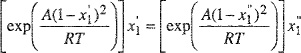
(E-9)

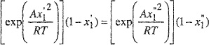
For a given A/RT, Eqs. (E-8) and (E-9) give a solution for and . (To be sure that and fall into the interval between zero and one, it is necessary that A/RT ≥ 2.)

We have just described how mutual solubilities may be found if the excess Gibbs energy is known. Frequently, however, it is desirable to reverse the procedure (i.e., to calculate excess Gibbs energy from known mutual solubilities) because it is often a relatively simple matter to obtain mutual solubilities experimentally.

To calculate excess Gibbs energy from measured and we must first choose a particular function for the excess Gibbs energy [Eq. (E-5)] containing no more than two unknown parameters, A and B. We can then find A and B by simultaneous solution of Eqs. (E-6) and (E-7). Once A and B are known, we can then calculate activity coefficients for both components in the two miscible regions. Therefore, mutual solubility data may be used to calculate vapor-liquid equilibria.³

³ However, A and B are functions of temperature.

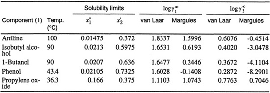
Calculation of excess Gibbs energies from mutual-solubility data is tedious but straightforward. The accuracy of such calculation is sensitive to the accuracy of the mutual solubility data but, even if these are highly accurate, the results obtained are likely to be only approximate because, without additional information, the estimated excess Gibbs energy function may contain no more than two parameters. Further, the results obtained depend strongly on the arbitrary algebraic function chosen to represent the excess Gibbs energy. This sensitivity is illustrated by calculations reported by Brian (1965)⁴ for five partially miscible binary systems shown in Table E-l. Using experimental mutual-solubility data, excess Gibbs energy parameters A and B were calculated once using the van Laar equation and once using the three-suffix Margules equation (see Sec. 6.10). With these parameters, Brian calculated activity coefficients at infinite dilution for both components. Although the same experimental data were used, results obtained with the van Laar equation differ markedly from those obtained with the Margules equation. Brian found that the differences are especially large in strongly asymmetric systems, i.e., in systems where the ratio / is far removed from unity. In the last system (propylene oxide/water), where this ratio is approximately 2, results obtained with the van Laar equation are close to those obtained with the Margules equation; however, for the system phenol/water, where the ratio is approximately 35, the limiting activity coefficient for water obtained with the van Laar equation is several orders of magnitude larger than that obtained with the Margules equation. Brian found that when predicted limiting activity coefficients were compared with experimental results, the Margules equation frequently gave poor results. The van Laar equation gave reasonable results but quantitative agreement with experiment was at best fair.

⁴ Similar calculations for aqueous systems are presented by D. L. Bergmaisn and C. E. Eckert, 1991, Fluid Phase Equilibria, 63: 141.

Table E-1 Limiting activity coefficients as calculated from mutual solubilities in five binary aqueous systems.

Renon found that the NRTL equation may be useful for calculating excess Gibbs energies from mutual solubility data. The NRTL equation [Eq. (6.11-6)] contains three parameters, but one of them, the nonrandomness parameter α₁₂, can often be estimated for a given binary mixture from experimental results for other mixtures of the same class. Once a value of aα₁₂ has been chosen,⁵ the two remaining parameters can be obtained from simultaneous solution of Eqs. (E-6) and (E-7).

⁵ Because these calculations are tedious, Renon (1969) has computer-programmed the equations of equilibrium and has presented the calculated results in graphical form.

For phase separation, α₁₂ may not exceed α_acrit that depends on mole fraction x₁ where splitting occurs and on β, the ratio of NRTL parameters τ₂₁ and τ₁₂. For several values of x₁ and β, α_crit has been calculated⁶ as shown in Table E-2.

⁶ Debenedetti and Reid (MIT), persona! communication.

Table E-2 Calculated α_crit for different values of x₁ and β

In mixtures with miscibility gaps, it is difficult to find an expression for the molar excess Gibbs energy g^E that yields simultaneously correct activity coefficients in the miscible region and correct activity coefficients at the solubility limits. To illustrate, Table E-3 compares observed solubility limits with those calculated from a two-parameter expression for g^E, where the parameters are evaluated from experimental data for activity coefficients at infinite dilution at the same temperature. Solubilities calculated with the van Laar equation or the UNIQUAC equation are in poor agreement with experiment. Table E-4 shows the reverse calculation: Experimental solubilities are used to determine two parameters in an expression for g^E that then yields limiting activity coefficients at the same temperature. Again, agreement with experiment is not good.

Table E-3 Solubility limits calculated from activity coefficients at infinite dilution using van Laar or UNIQUAC (Lobien, 1980, 1982).

Table E-4 Activity coefficients at infinite dilution calculated from solubility data using van Laar or UNIQUAC (Lobien, 1980, 1982)

It appears that, at present, for complex systems it is not possible to describe accurately both vapor-liquid and liquid-liquid equilibria using a simple expression for g^E containing only two adjustable binary parameters. To describe both kinds of equilibria, we probably need an expression for g^E that contains more than two binary parameters and, more important, some experimental data for both kinds of equilibria for evaluating these binary parameters.

Ternary (and higher) liquid-liquid equilibria. If an expression is available for relating molar excess Gibbs energy g^E to composition, the activity coefficient of every component is readily calculated as discussed in Sec. 6.3. For liquid-liquid equilibria in a system containing m components, there are m equations of equilibrium. Assuming that the standard-state fugacity for every component i in phase ′ is the same as that in phase ″, these equations are of the form indicated by Eq. (E-6), written m times, once for each component.

If an appropriate expression for g^E is available, it is not immediately obvious how to solve these m equations simultaneously when m > 2. To fix ideas, consider a ternary system at a fixed temperature and pressure. We want to know coordinates and on the binodal curve that are in equilibrium with coordinates and also on the connodal curve. (The line joining these two sets of coordinates is a tie line.) Therefore, we have four unknowns.⁷ However, there are only three equations of equilibrium. To find the desired coordinates, therefore, it is not sufficient to consider only the three equations indicated by Eq. (E-6). To obtain the coordinates, we must use a material balance by performing what is commonly known as an isothermal flash calculation.8

⁷ and are not independent unknowns because and .

⁸ For a discussion of adiabatic or isothermal flash calculations, see Praissnitz et al. (1980).

One mole of a liquid stream with overall composition x₁, x₂ is introduced into a flash chamber where that stream isothermally separates into two liquid phases ′ and ″. The number of rnoles of phases ′ and ″ are designated by L′ and L″. We can write three independent material balances:

(E-10)

(E-11)

(E-12)

We now have six equations that must be solved simultaneously: Three equations of equilibrium and three material balances. We also have six unknowns; they are , , , , L′, and L″. In principle, therefore, the problem is solved, although the numerical procedure for doing so efficiently is not necessarily easy. This flash calculation for a ternary system is readily generalized to systems containing any number of components. When m components are present, we have a total of 2m unknowns: 2(m – 1) compositions and two mole numbers, L′ and L″. These are found from m independent equations of equilibrium and m independent material balances.

To calculate ternary liquid-liquid equilibria at a fixed temperature, we require an expression for the molar excess Gibbs energy g^E as a function of composition;⁹ this expression requires binary parameters characterizing 1-2, 1-3, and 2-3 interactions. Calculated ternary equilibria are strongly sensitive to the choice of these parameters. The success of the calculation depends directly on the care exercised in choosing these binary parameters from data reduction.

⁹ At ordinary pressures and at conditions remote from critical, liquid-liquid equilibria are insensitive to the effect of pressure.

Unfortunately, realistic data reduction for a typical binary system cannot yield a unique set of binary parameters. To illustrate, consider data reduction for the system acetone (l)/methanol (2) reported by Anderson et al. (1978). Isobaric vapor-liquid equilibrium data have been obtained by Othmer at 1.006 bar; the variation in temperature is not large, from about 55 to 65°C. Using a statistical technique (the principle of maximum likelihood), Anderson fit Othmer’s data to the van Laar equation [Eq. (7-13)] and obtains

In his analysis of the data, Anderson took experimental error into account; for each measured quantity he assigned a variance: 0.003 bar for pressure, 0.2°C for temperature, 0.005 for liquid-phase mole fraction x, and 0.01 for vapor-phase mole fraction y.

In view of the experimental uncertainties and possible unsuitability of the van Laar model for representing the data, how much confidence can we have in the values A′ and B′? Are there other sets of parameters that can equally well represent the experimental data? Indeed there are, as was shown by Anderson; his calculations are summarized in Fig. E-l that shows permissible deviations in A′ and B′ at two confidence levels. The smaller ellipse (87% confidence limit) gives a region in the A′B′ plane wherein any point gives an “acceptable” set of A′ and B′ parameters; in this context, “acceptable” means that the vapor-liquid equilibria calculated with an acceptable A′, B′ set reproduce at least 87% of the experimental data to within the estimated experimental uncertainty.

Figure E-1 Data reduction for the system acetone (1)/methanol (2). Confidence ellipses for van Laar constants.

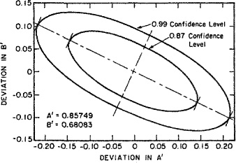
The elliptical form of the deviation plot indicates that the two parameters are correlated; i.e., parameters A′ and B′ are partially coupled. Having decided on one of the parameters, only a small variation is then permissible in the other.

In this example, the confidence ellipses are large because the data indicate appreciable random experimental error. The ellipses become smaller as the quality and/or quantity of the experimental data rises and as the suitability of the model for g^E increases. However, in practice, regardless of how good and plentiful the data are, and regardless of how suitable the model for g^E may be, there is always some ambiguity in the binary parameters. In practice, no set of binary data is completely free of error and no model is perfectly suitable. Therefore, it is not possible to specify a unique set of binary parameters.

To calculate phase equilibria for a ternary mixture, it is necessary to estimate binary parameters for each of the three binaries that constitute the ternary. Even if good experimental data are available for each of the binaries, there is always some uncertainty in the three sets of binary parameters. To obtain reliable calculated ternary liquid-liquid equilibria, the most important task is to choose the best set of binary parameters. This choice can only be made if a few ternary liquid-liquid data are available, as discussed, for example, by Bender and Block (1975), who used the NRTL equation, and by Anderson (1978a), who used the UNIQUAC equation.

To illustrate, consider the ternary system water (1)/TCE (2)/acetone (3)¹⁰ at 25°C. Water and TCE are only partially miscible, but the other two pairs are completely miscible. For the first pair, binary parameters are obtained from mutual solubilities and for the other pairs, from vapor-liquid equilibria. For the two completely miscible pairs, Bender and Block set NRTL parameters α₁₃ = α₂₃ = 0.3

¹⁰ TCE = 1,1,2-trichloroethane.

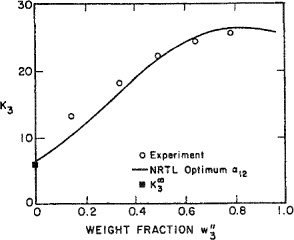
To optimize the fit of the ternary data, Bender and Block first adjusted τ₁₃, τ₃₁ and τ₂₃, τ₃₂, the NRTL parameters for the two miscible pairs. The adjustment was based on fitting the distribution coefficient of acetone at infinite dilution. Then Bender and Block adjusted α₁₂ to give good ternary tie lines. (Once α₁₂ is fixed, τ₁₂ and τ₂₁ immediately follow from the binary mutual solubility data.) Table E-5 gives NRTL parameters and Fig. E-2 compares calculated and experimental distribution coefficients for acetone.

Table E-5 Binary NRTL parameters used to calculate ternary liquid-liquid equilibria (Bender and Block, 1975).

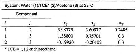
Figure E-2 Calculated and experimental distribution coefficients for acetone in the system water (1)/1,1,2-trichloroethane (2)/acetone (3). The distribution coefficient is defined with weight fractions.

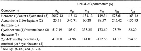
Anderson(1978) used the principle of maximum likelihood to obtain UNIQUAC binary parameters from data reduction; he used mutual-solubility data for partially miscible pairs and vapor-liquid equilibrium data for completely miscible pairs. In addition, he used a few (typically, one or two) ternary tie-line data. Figure E-3 shows calculated and experimental results for four ternary systems; the corresponding binary parameters are shown in Table E-6. No ternary (or higher) parameters are required because binary parameters were chosen with care, that is, with consideration of a few ternary data.

Figure E-3 Distribution of third component in four ternary systems.

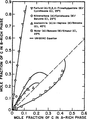
Table E-6 Binary UNIQUAC parameters used to calculate ternary liquid-liquid equilibria (Anderson, 1978a).

Anderson (1978a) also presented a procedure for calculating liquid-liquid equilibria in systems containing four (or more) components. When all binary parameters are chosen with care, it is often possible to calculate multicomponent liquid-liquid equilibria in good agreement with experiment.

An alternate procedure, presented by Cha (1985), includes a ternary correction factor in the expression for g^E, Like Anderson′s method, Cha′s requires some ternary liquid-liquid equilibrium data but because it includes ternary constants, calculated results are no longer highly sensitive to the choice of binary parameters.

References

Anderson, T. F., D. S. Abrams, and E. A. Grens, 1978, AIChE J., 24: 20.

Anderson, T. F. and J. M. Prausnitz, 1978a, Ind. Eng. Chem. Process Des. Dev., 17: 561.

Bender, E. and U. Block, 1975, Verfahrenstechnik, 9: 106.

Brian, P. L. T., 1965, Ind. Eng. Chem. Fundam., 4: 101.

Cha, H. and J. M. Prausnitz, 1985, Ind. Eng. Chem. Process Des. Dev,. 24: 551.

Lobien, G., 1980, Dissertation, University of California.

Lobien, G. and J. M. Prausnitz, 1982, Ind. Eng. Chem. Fundam,. 21: 109.

Prausnitz, J. M., T. F. Anderson, E. A. Grens, C. A. Eckert, R. Hsieh, and J. P. O’Connell, 1980, Computer Calculations for Multicomponent Vapor-Liquid and Liquid-Liquid Equilibria. Englewood Cliffs: Prentice-Hall.

Renon, H. and J. M. Prausnitz, 1969, Ind. Eng. Chem. Process Des. Dev,. 8: 413.