Chapter 10
Solubilities of Gases in Liquids

Numerous examples in nature illustrate the ability of liquids to dissolve gases; indeed, human life would not be possible if blood could not dissolve oxygen, nor could marine life exist if oxygen did not dissolve in water. Gas mixtures can be separated by absorption because different gases dissolve in a liquid in different amounts and therefore, most gaseous mixtures can be separated by contact with a suitable solvent that dissolves one gaseous component more than another. Further, knowledge of gas solubilities in water is important for describing processes that control the environmental distribution and ultimate fate of contaminants such as halogenated hydrocarbons (e.g. freons).

The solubility of a gas in a liquid is determined by the equations of phase equilibrium. If a gaseous phase and a liquid phase are in equilibrium, then for any component i the fugacities in both phases must be the same:

(10-1)

Equation (10-1) is of little use unless something can be said about how the fugacity of component i in each phase is related to the temperature, pressure, and composition of that phase. In Chap. 5 we discussed the fugacity of a component in the gaseous phase. In this chapter we consider the fugacity of a component i, normally a gas at the temperature under consideration, when it is dissolved in a liquid solvent.

10.1 The Ideal Solubility of a Gas

The simplest way to reduce Eq. (10-1) to a more useful form is to rewrite it in a manner suggested by Raoult’s law. In doing so, we introduce several drastic but convenient assumptions. Neglecting all gas-phase nonidealities as well as the effect of pressure on the condensed phase (Poynting correction),¹ and also neglecting any nonidealities due to solute-solvent interactions, the equation of equilibrium can be much simplified by writing

¹ see Sec. 3.3.

(10-2)

where p_i is the partial pressure of component i in the gas phase,² x_i is the solubility (mole fraction) of i in the liquid, and P_i^s is the saturation (vapor) pressure of pure (possibly hypothetical) liquid i at the temperature of the solution. The solubility x_i, as given in Eq. (10-2), is called the ideal solubility of the gas.

² The partial pressure p_i is, by definition, equal to the product of the gas-phase mole fraction and the total pressure: p_i = y_iP.

Aside from the severe simplifying assumptions made in obtaining Eq. (10.2), an obvious difficulty presents itself in finding a value for P_i^s, whenever (as is often the case) the solution temperature is above the critical temperature of pure i. In that case it has been customary to extrapolate the saturation pressure of pure liquid i beyond its critical temperature to the solution temperature; the saturation pressure of the hypothetical liquid is usually found from a straight-line extrapolation on a semilogarithmic plot of saturation pressure versus reciprocal absolute temperature as shown in Fig. 10-1. The use of these particular coordinates does not have any sound theoretical basis but is dictated by convenience.

The ideal solubility, as calculated by Eq. (10-2) and the extrapolation scheme indicated in Fig. 10-1, usually gives correct order-of-magnitude results provided the partial pressure of the gas is not large and provided the solution temperature is well below the critical temperature of the solvent and not excessively above the critical temperature of the gaseous solute. In some cases, where the physical properties of solute and solvent are similar (e.g., chlorine in carbon tetrachloride), the ideal solubility is remarkably close to the experimental value.

Figure 10-1 Convenient but arbitrary extrapolation of liquid saturation pressure into the hypothetical liquid region.

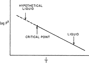
Table 10-1 compares ideal and observed solubilities of four gases in a number of solvents at 25°C and 1.013 bar partial gas pressure. The ideal solubility is significantly different from observed solubilities, but it is of the right order of magnitude.

Table 10-1 Solubilities (mole fraction × 10⁴) of gases in several liquid solvents at 25°C and 1.013 bar partial pressure.

The ideal solubility given by Eq. (10-2) suffers from two serious defects. First, it is independent of the nature of the solvent; Eq. (10-2) says that a given gas, at a fixed temperature and partial pressure, has the same solubility in all solvents. This conclusion is contrary to observation as illustrated by the data in Table 10-1. Second, Eq. (10-2), coupled with the extrapolation scheme shown in Fig. 10-1, predicts that at constant partial pressure, the solubility of a gas always decreases with rising temperature. This prediction is frequently correct but not always; near room temperature the solubilities of the light gases helium, hydrogen, and neon increase with rising temperature in most solvents, and at somewhat higher temperatures the solubilities of gases like nitrogen, oxygen, argon, and methane also increase with rising temperature in many common solvents. Because of these two defects, the ideal-solubility equation has severely limited applicability, it should be used only whenever no more is desired than a rough estimate of gas solubility.

10.2 Henry’s Law and Its Thermodynamic Significance

It was observed many years ago that the solubility of a gas in a liquid is often proportional to its partial pressure in the gas phase, provided that the partial pressure is not large. The equation that describes this observation is commonly known as Henry’s law:

(10-3)

where, for any given solute and solvent, k is a constant of proportionality depending only on temperature.³ Equation (10-3) always provides an excellent approximation when the solubility and the partial pressure of the solute are small and when the temperature is well below the critical of the solvent. Just how small the partial pressure and solubility have to be for Eq. (10-3) to hold, varies from one system to another, and the reasons for this variation will become apparent later. In general, however, as a rough rule for many common systems, the partial pressure should not exceed 5 or 10 bar and the solubility should not exceed about 3 mol %; however, in those systems where solute and solvent are chemically highly dissimilar (e.g., systems containing helium or hydrogen) large deviations from Eq. (10-3) are frequently observed at much lower solubilities. On the other hand, in some systems (e.g., carbon dioxide/benzene near room temperature), Eq. (10-3) appears to hold to large partial pressures and solubilities, but such cases are rare; the apparent validity of Eq. (10-3) at large solubilities is usually fortuitous due to cancellation of two (or more) factors that, taken separately, would cause that equation to fail.

³ For a given binary system, Henry’s constant H_2,1 depends on temperature and, to a lesser degree, on total pressure, as discussed in Sec. 10.3. A precise definition of H_2,1 is given by Eq. (6-31) or Eq. (10-9).

The assumptions leading to Eq. (10-3) can readily be recognized by comparing it with Eq. (10-1). A comparison of the left-hand sides shows that in Henry’s law the gas phase is assumed to be ideal and thus the fugacity is replaced by the partial pressure; this simplification can be avoided by the methods discussed in Chap. 5. A comparison of the right-hand sides shows that the fugacity in the liquid phase is assumed to be proportional to the mole fraction and that the constant of proportionality is taken as an empirical factor that depends on the natures of solute and solvent and on the temperature. The thermodynamic significance of this constant can be established by comparing the liquid fugacity as given by Henry’s law with that obtained in the more conventional manner using the concept of an activity coefficient γ and some standard-state fugacity f⁰:

(10-4)

Thus,

(10-5)

where 1 stands for solvent and 2 stands for solute.

At a given temperature and pressure, the standard-state fugacity is a constant and does not depend on the solute mole fraction in the liquid phase. Since k does not depend on x₂, it follows from Eq. (10-5) that the activity coefficient γ₂ must also be independent of x₂; it is this feature, the constancy of the activity coefficient, which contains the essential assumption of Henry’s law.

The activity coefficient of a solute is nearly independent of the solute’s mole fraction provided the latter is sufficiently small. This can be shown from simple mathematical considerations. To fix ideas, take the case where γ₂ is normalized to approach unity as the mole fraction of 2 goes to unity. As shown in Chap. 6, it is convenient to express In γ₂ as a power series in (1 -x₂):

(10-6)

where A, B,… are constants depending on temperature and on intermolecular forces between solute and solvent. Equation (10-6) shows at once that if x₂ << 1, then γ₂ is only weakly dependent on x₂ and Henry’s law provides a good approximation.

Equation (10-6) gives some insight into the well-known observation that Henry’s law is a good approximation to relatively large solubilities for some systems but fails for relatively small solubilities in other systems. Consider the case where only the first term in the series is retained, while higher terms are neglected. Coefficient A is a measure of nonideality; if A is positive, it indicates the “dislike” between solute and solvent, whereas if it is negative, its absolute value may be a measure of the tendency between solute and solvent to form a complex. In any case, it is the absolute value of A/RT that determines the range of validity of Henry’s law; in the limit, if A/RT = 0 (ideal solution), Henry’s law holds for the entire range of composition 0 ≤ x₂ ≤ 1. If A/RT is small compared to unity, then activity coefficient γ₂ does not change much even for appreciable x₂, but if it is large, then even a small x₂ can produce a significant change in the activity coefficient with composition. In the limit as x₂ approaches zero, the logarithm of the activity coefficient approaches the constant value A/RT, and therefore Henry’s law is valid as a limiting relation.

As indicated by Eq. (10-3), Henry’s law assumes that the gas-phase fugacity is equal to the partial pressure. This assumption is not necessary and is easily removed by including the gas-phase fugacity coefficient φ as discussed in detail earlier; more properly, therefore, Henry’s law for solute i is

(10-7)

Table 10-2 presents experimental Henry’s constants for four gases in ethylene oxide at three temperatures. These results were calculated from experimental solubility data and from volumetric data shown in Table 10-3. The second virial coefficients are needed to calculate vapor-phase fugacity coefficients and the liquid-phase partial molar volumes of the solutes at infinite dilution are needed to correct for the effect of pressure, as discussed in the next section.

Table 10-2 Henry’s constants (bar) for four gases in ethylene oxide.*

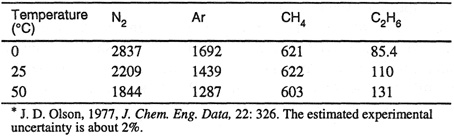
Table 10-3 Some volumetric properties of four ethylene oxide (1)/gas (2) systems.*

10.3 Effect of Pressure on Gas Solubility

In the preceding section we discussed the essential assumption in Henry’s law, i.e., that at constant temperature, the fugacity of solute i is proportional to the mole fraction x_i. The constant of proportionality H_{i, solvent} is not a function of composition but depends on temperature and, to a lesser degree, pressure. The pressure dependence can be neglected as long as the pressure is not large. At high pressures, however, the effect is not negligible and therefore it is necessary to consider how Henry’s constant depends on pressure. This dependence is easily obtained by using the exact equation

(10-8)

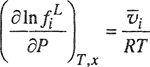
where is the partial molar volume of i in the liquid phase. The thermodynamic definition of Henry’s constant is

(10-9)

Substitution of Eq. (10-9) into Eq. (10-8) gives

(10-10)

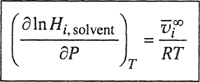
where ^∞ is the partial molar volume of solute i in the liquid phase at infinite dilution.⁴ Integrating Eq. (10-10) and assuming, as before, that the fugacity of i at constant temperature and pressure is proportional to x_i, we obtain a more general form of Henry’s law:

⁴ see Sec. 12.4 for a discussion of liquid-phase partial molar volumes.

(10-11)

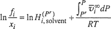
where is Henry’s constant evaluated at an arbitrary reference pressure P^r. As x_i → 0, the total pressure is P₁^s, the saturation (vapor) pressure of the solvent; it is often convenient, therefore, to set P^r = P^s₁.

If the solution temperature is well below the critical temperature of the solvent, it is reasonable to assume that ^∞ is independent of pressure. Letting subscript 1 refer to the solvent and subscript 2 to the solute, Eq. (10-11) becomes

(10-12)

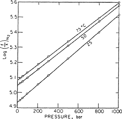
Equation (10-12) is the Krichevsky-Kasarnovsky equation (1935), although its first clear derivation was given by Dodge and Newton (1937). This equation is remarkably useful for representing solubilities of sparingly soluble gases to very high pressures. Figures 10-2 and 10-3 show that solubility data for hydrogen and nitrogen in water to 1000 bar are accurately reproduced by the Krichevsky-Kasarnovsky equation; in this case, the vapor pressure of the solvent is negligible in comparison to the total pressure and therefore the abscissa reads P rather than P-P₁^s. The intercepts of these plots give , and the slopes yield the partial molar volumes of the gaseous solutes in the liquid phase. At 25°C, Figs. 10-2 and 10-3 give partial molar volumes; that for hydrogen is 19.5 and that for nitrogen is 32.8 cm³ mol^-1. These results are in fair agreement with partial molar volumes for these gases in water obtained from dilatometric measurements. In his detailed studies of gas solubilities in amines and in alcohols, Brunner (1978, 1979) has shown that Eq. (10-12) gives an excellent representation of the experimental data at high pressures.

Figure 10-2 Solubility of hydrogen in water at high pressures.

Figure 10-3 Solubility of nitrogen in water at high pressures.

Equation (10-12) can be expected to hold for all those cases that conform to the two assumptions on which the equation rests. One of these is that the activity coefficient of the solute does not change noticeably over the range of x₂ considered; in other words, x₂ must be small, as discussed in the preceding section. The other assumption states that the infinitely dilute liquid solution must be essentially incompressible, very nearly correct at temperatures far removed from the critical temperature of the solution.

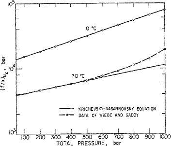
To illustrate the use and limitation of the Krichevsky-Kasarnovsky equation, consider the high-pressure solubility data (Wiebe and Gaddy, 1937) for nitrogen in liquid ammonia. These are shown in Fig. 10-4 plotted in the manner indicated by Eq. (10-12). At 0°C, the Krichevsky-Kasarnovsky equation holds to 1000 bar, but at 70°C it breaks down after about 600 bar. This striking difference is readily explained upon considering the two assumptions just mentioned; at 0°C liquid ammonia is an unexpanded liquid solvent (the critical temperature of ammonia is 132.3°C) and the solubility of nitrogen is small throughout, only 2.2 mol % at 1000 bar. At 0°C, therefore, the assumptions of Eq. (10-12) are reasonably satisfied. However, at 70°C liquid ammonia is already quite expanded (and compressible) aad the solubility of nitrogen is no longer small, 12.9 mol % at 1000 bar. Under these conditions, it is not reasonable to expect that the activity coefficient of nitrogen in the liquid phase is independent of composition, nor is it likely that the partial molar volume is constant. As a result, it is not surprising that the Krichevsky-Kasaraovsky equation gives an excellent representation of the data for the entire pressure range at 0°C but fails at higher pressures for the data at 70°C.

Figure 10-4 Success and failure of the Krichevsky-Kasarnovsky equation. Solubility of nitrogen in liquid ammonia.

Variation of the activity coefficient of the solute with mole fraction can be taken into account by one of the methods discussed in Chap. 6. In the simplest case we may assume that the activity coefficient of the solvent is given by a two-suffix Margules equation:

(10-13)

where A is an empirical constant determined by intermolecular forces in the solution. Typically, A is a weak function of temperature.

The activity coefficient γ₂^* of the solute, normalized according to the unsymmetric convention (see Sec. 6.4), is then found from the Gibbs-Duhem equation; it is given by

(10-14)

The fugacity of component 2 at pressure P^s₁ is

(10-15)

and instead of Eq. (10-12) we obtain:⁵

⁵ Equation (10-16) assumes that the partial molar volume of the solute is independent of pressure and composition over the pressure and composition ranges under consideration.

(10-16)

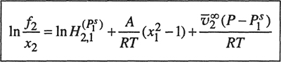
Equation (10-16) is the Krichevsky-Ilinskaya equation (1945). Because of the additional parameter, it has a wider applicability than does Eq. (10-12). It is especially useful for solutions of light gases (such as helium and hydrogen) in liquid solvents where the solubility is appreciable. For example, Orentlicher (1964) found that Eq. (10-16) could be used to correlate solubility data for hydrogen in a variety of solvents at low temperatures and at pressures to about 100 bar. Table 10-4 gives parameters reported by Orentlicher, In the systems studied, the solubility of hydrogen may be as large as 20 mol % and therefore the data could not be adequately represented by the simpler Krichevsky-Kasarnovsky equation.

Table 10-4 Thermodynamic parameters for correlating hydrogen solubilities.*

When, for a given temperature, gas-solubility data alone are available as a function of pressure, it is difficult to obtain three isothermal parameters (, , and A) from data reduction. When ln(f₂/x₂) is plotted versus (P-P^s₁), the intercept can give a good value for but, since the slope depends on both correction terms in Eq. (10-16), it is often not possible to obtain unique values for and A from gas-solubility data alone. Some other information is needed to establish all three parameters in Eq. (10-16). In the absence of pertinent experimental information, it is possible to use an equation of state as discussed below.

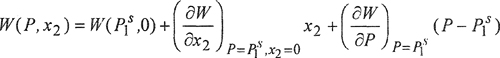
Let W = ln(f₂/x₂) and consider isothermal changes in W in the region P = P^s₁ and x₂ = 0. At a constant temperature T, we write a Taylor series:

(10-17)

Comparison with Eq. (10-16) shows that

(10-18)

(10-19)

and

(10-20)

We can calculate parameters , and A from an equation of state. First,

(10-21)

where is the fugacity coefficient of solute 2 in the liquid phase at temperature T, at infinite dilution (x₂ = 0), and at liquid molar volume , the saturated molar volume of the solvent at T,

Second, from elementary calculus,

(10-22)

where n is the number of moles and V is the total volume (see Chap. 3). Finally,

(10-23)

If a reliable equation of state is available for the dilute mixture, the three Krichevsky-Ilinskaya parameters can be calculated. To do so, it is necessary that the equation of state be valid for the entire density range, from zero to ()^-1, because (see Chap. 3) fugacity coefficients depend on an integral of the equation of state.

As discussed in other chapters, calculated thermodynamic properties of mixtures often depend strongly on the mixing rules and especially on the cross term for the characteristic energy parameter. For example, in equations of the van der Waals form, the constant a (for a binary mixture) is usually written

(10-24)

where k₁₂ is a binary parameter that has a large effect on , especially when x₂ is small.

For some given equation of state, the important binary parameter k₁₂ can be found from the experimentally determined Henry’s constant or vapor-liquid equilibrium data, using Eq. (10-21); parameter k₁₂ is adjusted until the calculated fugacity coefficient satisfies Eq. (10-21). Once k₁₂ is known, it may also be used to calculate parameters and A. Therefore, with the help of an equation of state, gas-solubility data at low pressures () may be used to calculate gas solubilities at higher pressures. While such calculations can be done directly (see Chaps. 3 and 12) without an equation such as that of Krichevsky-Ilinskaya, the procedure outlined here shows the direct correspondence between one method, based on an activity coefficient, and another, based on an equation of state. Bender et al. (1984) have presented some examples of this correspondence. Using the Redlich-Kwong (or Peng-Robinson) equation of state, Bender et al. showed that calculated and observed high-pressure gas solubilities are in good agreement for hydrogen in ethylene diamine and for methane in n-hexane.

Another example of this procedure is provided by solubility data for carbon dioxide in phenol (Yau et al., 1992) at 75, 100, 125, and 150°C shown in Fig. 10-5. The equation of state used was that of Redlich-Kwong-Soave (see Sec. 12.8); for each isotherm, interaction parameter k₁₂ was obtained from regression of vapor-liquid equilibrium data for the same binary system. Table 10-5 gives the resulting thermodynamic parameters for carbon-dioxide solubility in phenol, , , and A, as obtained from Eqs. (10-21), (10-22), and (10-23), respectively. As Fig. 10-5 shows, with the parameters listed in Table 10-5, the Krichevsky-Ilinskaya equation [Eq. (10-16)] represents well the experimental data over the entire temperature and pressure range studied.

Figure 10-5 Solubility of carbon dioxide in phenol. Solid lines are calculated from the Krichevsky-ilinskaya equation [Eq. (10-16)] with the parameters feted in Table 10-5 for the Redlich-Kwong-Soave equation of state. Experimental data from Yau et al. (1992).

Table 10-5 Thermodynamic parameters for correlating carbon dioxide solubility in phenol. Parameter k₁₂ was obtained from regression of vapor-liquid equilibrium data for the carbon dioxide/phenol system at each isotherm.

10.4 Effect of Temperature on Gas Solubility

Many elementary textbooks on chemistry state, without qualification, that as the temperature rises, gas solubility falls. While this statement is often correct, there are many cases where it is not, especially at high temperatures where it is more common for gas solubility to increase with rising temperature.

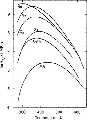
No simple generalizations can be made concerning the effect of temperature on solubility as indicated by Fig. 10-6 that shows Henry’s constants as a function of temperature for nine binary systems. Not only does Henry’s constant vary significantly from one system to another but, equally striking, the effect of temperature depends strongly on the properties of the particular system and also on the temperature.

Figure 10-6 Henry’s constants (bar) for typical gases range over five orders of magnitude. The effect of temperature differs qualitatively from one system to another.

The temperature derivative of the solubility, as calculated from the Gibbs-Helmholtz equation,⁶ is directly related to either the partial molar enthalpy or the partial molar entropy of the gaseous solute in the liquid phase. Therefore, if something can be said about the enthalpy or entropy change of solution, insight can be gained on the effect of temperature on solubility. A general derivation of the thermodynamic relations is given elsewhere (Hildebrand and Scott, 1962; Sherwood, 1962); we consider here only the relatively simple case where the solvent is essentially nonvolatile and where the solubility is sufficiently small to make the activity coefficient of the solute independent of the mole fraction. With these restrictions, it can be shown that

⁶ See Eq. (6-12).

(10-25)

and

(10-26)

where x₂ is the mole fraction of gaseous solute at saturation and

where and are, respectively, the enthalpy and the entropy of pure 2 gas, at system temperature and pressure.

First, we consider Eq. (10-26); if the partial molar entropy change of the solute is positive, then the solubility increases with rising temperature; otherwise, it falls. To understand the significance of the entropy change, it is convenient to divide it into two parts:

(10-27)

where is the entropy of the (hypothetical) pure liquid at the temperature of the solution. The first term OB the right-hand side of Eq. (10-27) is (essentially) the entropy of condensation of the pure gas and, in general, we expect this term to be negative because the entropy (disorder) of a liquid is lower than that of a saturated gas at the same temperature. The second term is the partial molar entropy of solution of the condensed solute and, assuming ideal entropy of mixing for the two liquids, we can write

(10-28)

Because x₂ < 1, the second term in Eq. (10-27) is positive and the smaller the solubility, the larger this term. It therefore follows that should be positive for those gases that have very small solubilities and negative for the others; this result leads to the expectation that sparingly soluble gases (very small x₂) show positive temperature coefficients of solubility, whereas readily soluble gases (relatively large x₂) show negative temperature coefficients. This expectation is observed. This semiquantitative interpretation of the sign of is in good agreement with observed behavior of gas-liquid solutions as shown in Fig. 10-7 where the observed partial molar entropy change [Eq. (10-26)] is related to the ideal partial molar entropy of the condensed solute [Eq. (10-28)]. The plot gives experimental results at 25°C for 14 gases in six solvents at 1.013 bar partial pressure. The figure can be divided into two parts: the upper part corresponds to a positive, and the lower to a negative temperature coefficient of solubility.

Figure 10-7 Entropy of solution of gases in liquids as a function of gas solubility (mote fraction) x₂ at 25°C and 1.013 bar (Hildebrand and Scott, 1962). Units of entropy and gas constant R are J mol^-1 K^-1.

As suggested by the foregoing discussion, Fig. 10-7 shows that, as a general rule, the solubility of a gas rises with increasing temperature whenever x₂ is small (–Rlnx₂ is large), and it falls with increasing temperature whenever x₂ is large (–Rlnx₂ is small). This is only a general rule, and there are differences in behavior between different gases and different solvents. For example, consider the solubility that a gas must have to exhibit a zero temperature coefficient of solubility (no change in solubility with temperature). In perfluoroheptane (C₇F₁₆), is zero when –Rlnx₂ = 47.3 J mol^-1 K^-1; therefore, in this solvent the temperature coefficient of solubility changes sign when x₂ = 3.43×10^-3. In carbon disulfide, however, the corresponding value is x₂ = 0.76×l0^-3. Going from left to right, the solvents in Fig. 10-7 are arranged in order of decreasing solubility parameters. At constant solubility (i.e., constant x₂), the temperature coefficient of solubility for a given gas has a tendency to increase (algebraically) as the solubility parameter of the solvent falls.

Some qualitative insight into the effect of temperature on gas solubility can also be obtained from the partial molar enthalpy change [Eq. (10-25)]. It is useful to divide this change into two parts:

(10-29)

where is the enthalpy of the (hypothetical) pure liquid at the temperature of the solution.

The first term in Eq. (10-29) is (essentially) the enthalpy of condensation of pure solute and, because the enthalpy of a liquid is generally lower than that of a gas at the same temperature, we expect this quantity to be negative.⁷ The second quantity is the partial enthalpy of mixing for the liquid solute; in the absence of solvation between solute and solvent, this quantity tends to be positive (endothermic) and the theory of regular solutions (Chap. 7) tells us that the larger the difference between the cohesive energy density of the solute and that of the solvent, the larger the enthalpy of mixing. If this difference is very large (e.g., hydrogen and benzene), the second term in Eq. (10-29) dominates; is then positive and the solubility increases with rising temperature. However, if the difference in cohesive energy densities is small (e.g., chlorine in carbon tetrachloride), the first term in Eq. (10-29) dominates; is then negative and the solubility falls as temperature increases.

⁷ At T/T_c2 >> 1, ( – ) may be positive. See, for example, G. J. F. Breedveld and J. M. Prausnitz, 1973, AIChE J., 19: 783, where it is shown that, at very high reduced temperatures, an isothermal increase in the volume of a Said may lower its enthalpy.

If there are specific chemical interactions between solute and solvent (e.g., ammonia and water), then both terms in Eq. (10-29) are negative (exothermic) and the solubility decreases rapidly as the temperature rises.

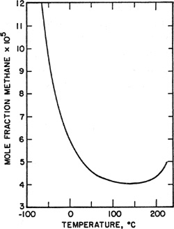
The effect of temperature on solubility is sensitive to the intermolecular forces of the solute-solvent system. When the partial pressure of the solute is small, the solubility typically decreases with temperature, goes through a minimum, and then rises. To illustrate, Fig. 10-8 shows the solubility of methane in n-heptane over a wide temperature range. For most common systems the temperature corresponding to minimum solubility lies well above room temperature but for light gases, minimum solubility is often observed at low temperatures.

Figure 10-8 Solubility of methane in n-heptane when the vapor-phase fugacity of methane is 0.01 bar.

A thorough study of the solubilities of simple gases in water from 0 to 50°C has been reported by Benson and Krause (1976). Theoretical and empirical evidence show that, although other expressions may provide reasonable approximations, the effect of temperature on Henry’s constant over narrow temperature ranges is best given by an equation of the form

(10-30)

Here, H_2,1 is Henry’s constant (in bar) for solute 2 in solvent 1 (water); α₂ and T₂ are constants specific to the solute. For simple gases, β is a universal constant. Equation (10-30) is based primarily on experimental data in the region 0 to 50°C.

Table 10-6 reports constants α₂ and T₂ for seven solutes; these, in turn, can be related to physical properties of the solute. It is clear from Eq. (10-30) that T₂ is the temperature where H_2,1 is 1 atm. When H_2,1 is expressed in atmospheres, T₂ is the normal boiling point of a hypothetical liquid, a condensed solute where each solute molecule is completely surrounded by water. Equation (10-30) gives good results for the partial entropy and enthalpy of solution and, most impressive, for the partial heat capacity of the solute. Therefore, while Eq. (10-30) appears, in essence, to be little more than a concise summary of a large body of high-quality experimental data, it may be useful as a guide toward theoretical understanding of dilute aqueous solutions of nonelectrolytes. To appreciate the possible theoretical significance of this equation, it is necessary to consult the detailed paper by Benson and Krause. It is nevertheless quoted here to point out once again that phase-equilibrium thermodynamics progresses most rapidly when good experimental data are analyzed with attention to primary as well as derivative thermodynamic properties⁸ and with ever-open eyes toward establishing connections between theory and experiment.

⁸ In this case, the primary property is Henry’s constant; the derivative properties are partial molar enthalpy and entropy (first derivative) and partial molar heat capacity (second derivative).

Table 10-6 Parameters for Eq. (10-30) (with β = 36.855) giving Henry’s constants (in bar) for seven gaseous solutes in water in the region 0 to 50°C (Benson and Krause, 1976).

Over a wider range of temperatures, simple equations such as Eq. (10-30) are unable to describe Henry’s constant. Harvey (1996) developed a semiempirical correlation of Henry’s constants over large temperature ranges. To illustrate, Fig. 10-9 shows Henry’s constants for six nonpolar gases in water as a function of temperature obtained from Harvey’s correlation. In addition to the maximum (corresponding to the minimum solubility), a striking feature is the significant decrease in Henry’s constant as the critical temperature of water (647.1 K) is approached.

Figure 10-9 Henry’s constants H_2,1 for several gases In water. Curves represent data fitted by the correlation of Harvey (1996).

The behavior of Henry’s constant near the solvent critical point has been a source of confusion (for example, erroneous suggestions that H _2,1 approaches zero or a constant for al! solutes in this limit), but it is now understood well. Beutier and Renon (1978) showed that, at the critical point of solvent 1, Henry’s constant for solute 2 is given by H _2,1=P_c1φ^∞₂ where P_c1 is the solvent’s critical pressure and φ₂^∞ is the solute fugacity coefficient at infinite dilution at the critical temperature and pressure of the solvent. The derivative dH_2,1/dT diverges to negative infinity (or positive infinity for some solute/solvent pairs) due to the diverging compressibility of the solvent.

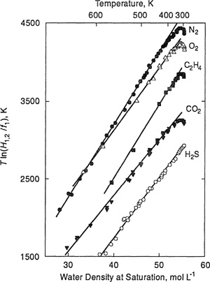
Japas and Levelt Sengers (1989) derived the correct functional form for this divergence. Near the solvent’s critical point, a function of Henry’s constant is linear in density:

(10-31)

where f₁ and ρ₁ are, respectively, the fugacity and the density of the pure solvent and ρ_c1 is the solvent’s critical density. In Eq. (10-31), constant A is related to H_2,1 at the solvent’s critical-point as determined by φ₂^∞; and constant B is related to a thermodynamic derivative called the Krichevsky parameter (see, e.g. Levelt Sengers, 1991), the key quantity describing dilute mixtures near the solvent’s critical point. Japas and Levelt Sengers have also derived a linear relationship for the infinite dil ution partition coefficient K^∞,

(10-32)

where is the saturated liquid density of the solvent and K^∞ is defined along the solvent’s coexistence curve by

(10-33)

While Eqs. (10-31) and (10-31) are only asymptotic results, they describe experimental data over a wide range of conditions. Figure 10-10 shows Henry’s-constant data for several solutes in water plotted according to Eq. (10-31). The data display striking linearity (more than one has a right to expect from a result derived only near the critical point) from near-critical temperatures to approximately 100°C.

Figure 10-10 Henry’s constants for several gases in water plotted according to Eq. (10-31).

Although we do not fully understand the reason for such extended linear behavior, it can be used to develop correlations, for example, for Henry’s constants (Harvey and Levelt Sengers, 1990; Harvey, 1996) and for infinite-dilution partition coefficients (Alvarez et al., 1994). Because these correlations are "anchored" with the correct near-critical functional form, they can be extrapolated to high temperatures with more confidence than empirical fitting equations. These results demonstrate how we can improve correlations by choosing the proper independent variable (here solvent density) and making reasonable use of theoretical boundary conditions.

10.5 Estimation of Gas Solubility

Reliable data on the solubility of gases in liquids are not plentiful, especially at temperatures well removed from 25 °C. Hildebrand and coworkers have obtained a large amount of accurate data in the vicinity of room temperature and therefore we consider first the semiempirical correlations they have established.

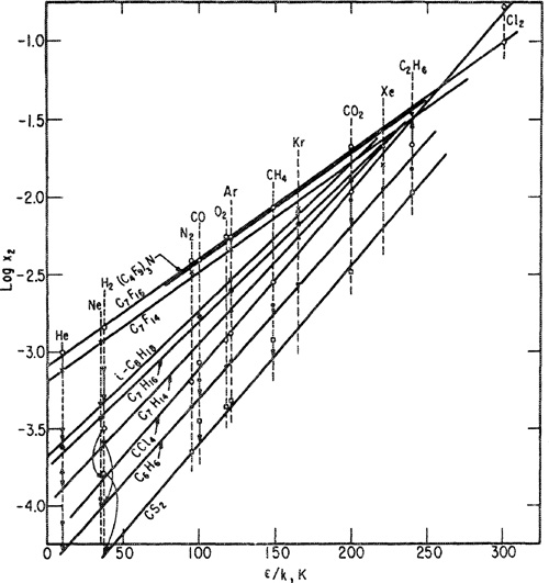
Figure 10-11 shows solubilities of 12 gases (at 25°C and 1.013 bar partial pressure) as a function of the solubility parameter of the solvent, and Fig. 10-12 shows solubilities of 13 gases (at the same conditions) in nine solvents as a function of Lennard-Jones energy parameters (ε/K) determined from second-virial-coefficient data for the solutes. These plots, presented by Hildebrand and Scott (1962), indicate that the solubilities of nonpolar gases in nonpolar solvents can be correlated in terms of two parameters: the solubility parameter of the solvent and the Lennard-Jones energy parameter for the solute. Figures 10-11 and 10-12, therefore, may be used with some confidence to predict solubilities in nonpolar systems where no experimental data are available; these predictions are necessarily limited to systems at 25°C, but with the help of Eq. (10-26) and the entropy data shown In Fig. 10-7, it is possible to predict solubilities at other temperatures not far removed from 25°C.

Figure 10-11 Solubilities of gases in liquids at 25°C and at a partial pressure of 1.013 bar as a function of solvent solubility parameter δ1 (Hildebrand and Scott, 1962).

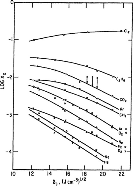
Figures 10-11 and 10-12 are useful, but in addition to their utility we must recognize that even for nonpolar systems at one temperature there are significant deviations from "regular" behavior; the straight lines correlate most of the experimental results but there are notable exceptions. In Fig. 10-11 the solubilities of carbon dioxide in benzene, toluene, and carbon tetrachloride are somewhat larger than those predicted from results obtained in other solvents. The high solubility in aromatic hydrocarbons can probably be attributed to a Lewis acid-base interaction between acidic carbon dioxide and the basic aromatic; apparently there is also some specific chemical interaction between carbon dioxide and carbon tetrachloride that may be related to carbon dioxide’s quadrupole moment. In Fig. 10-12 the solubilities of the quantum gases, helium, hydrogen, and neon, are a little higher than expected, the discrepancies becoming larger as the solubility parameter of the solvent increases. These anomalies are not yet fully understood.⁹

⁹ Refinements in regular-solution theory for correlating gas solubilities are discussed by J. H. Hildebrand and R. H. Lamoreaux, 1974, Ind. Eng. Chem. Fundam., 13: 110 and by R. G. Linford and D. G. T. Thomhill, 1977J. Appl Chem. Bioteclwol., 27: 479. Unfortunately, these refinements are confined to temperatures near 25°C.

Figure 10-12 Solubilities of gases in liquids at 25°C and at a partiai pressure of 1.013 bar as a function of solute characteristic ε/k (Lennard-Jones 6-12-potential) (Hirschfelder et al., 1954).

Hildebrand’s correlations provide a good basis for estimating gas solubilities in nonpolar systems at temperatures near 25°C but, since the entropy of solution is temperature-dependent, these correlations are not helpful at temperatures well removed from 25°C. Unfortunately, solubility data at temperatures much larger or smaller than room temperature are scarce and therefore, strictly empirical correlations cannot be used; rather, it is necessary to resort to whatever theoretical methods might be available and appropriate.

A rigorous method for the prediction of gas solubilities requires a valid theory of solutions. While efforts toward such a theory are progressing,¹⁰ they have not yet reached a stage for practical applications. For a semitheoretical description of nonpolar systems, the theory of regular solutions and the theorem of corresponding states can serve as the basis for a correlating scheme (Prausnitz and Shair, 1961) that we now describe.

¹⁰ See, for example, L. Lue and D. Blankschtein, 1992, J. Pkys. Chem., 96: 8582, who use the integral-equation theory of fluids for describing the solubilities of gases in water.

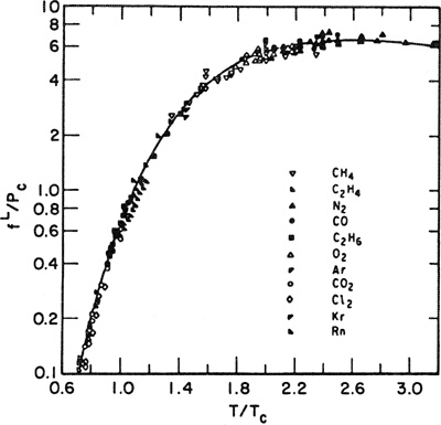
Consider a gaseous component at fugacity f^G₂ dissolved isothermally in a liquid not near its critical temperature. The solution process is accompanied by a change in enthalpy and in entropy, as occurs when two liquids are mixed. However, in addition, the solution process for the gas is accompanied by a large decrease in volume because the partial molar volume of the solute in the condensed phase is much smaller than that in the gas phase. This large decrease in volume distinguishes solution of a gas in a liquid from solution of another liquid or of a solid. Therefore, to apply regular solution theory (that assumes no volume change), it is necessary first to “condense” the gas to a volume close to the partial molar volume that it has as a solute in a liquid solvent. The isothermal solution process of the gaseous solute is then considered in two steps, I and II:

(10-34)

(10-35)

(10-36)

where is the fugacity of (hypothetical) pure liquid solute and γ2 is the symmetrically normalized activity coefficient of the solute referred to the (hypothetical) pure liquid (γ₂ → 1 as x₂ → 1)

In the first step, the gas isothermally “condenses” to a hypothetical state having a liquid-like volume. In the second step, the hypothetical, liquid-like fluid dissolves in the solvent. Since the solute in the liquid solution is in equilibrium with the gas that is at fugacity f₂^G, the equation of equilibrium is

(10-37)

We assume that the regular-solution equation gives the activity coefficient for the gaseous solute:¹¹

¹¹ see Sec. 7.2 for a discussion of the tegular-solution equation. A list of liquid molar volumes and solubility parameters for some common solvents is given in Table 7-1.

(10-38)

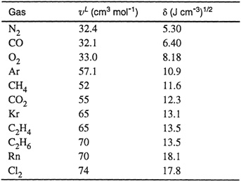
where δ₁ is the solubility parameter of solvent, δ₂ is the solubility parameter of solute, is the molar “liquid” volume of solute, and Φ₁ is the volume fraction of solvent.

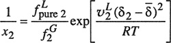
Substitution of Eqs. (10-34), (10-35), (10-36), and (10-38) into Eq. (10-37) gives the solubility:

(10-39)

Equation (10-39) forms the basis of the correlating scheme; it requires three parameters for the gaseous component as a hypothetical liquid: the pure liquid fugacity, the liquid volume, and the solubility parameter. These parameters are all temperature dependent; however, the theory of regular solutions assumes that at constant composition

(10-40)

and therefore, the quantity (δ₁-δ₂)²Φ²₁; is not temperature-dependent. As a result, any convenient temperature may be used for and δ₂ provided that the same temperature is also used for δ₁ and (The most convenient temperature, that used here, is 25°C.) The fugacity of the hypothetical liquid, however, must be a function of temperature.

The three correlating parameters for the gaseous solutes were calculated (Prausnitz and Shair, 1961) from experimental solubility data. The molar volume and the solubility parameter δ₂, both at 25°C, are given for 11 gases in Table 10-7. However, as explained above, Eq. (10-39) is not restricted to 25°C; in principle, it may be used at any temperature provided that it is well removed from the critical temperature of the solvent. A correlation similar to that of Shair has been given by Yen and McKetta (1962).

Table 10-7 “Liquid” volumes and solubility parameters for gaseous solutes at 25°C.

For nonpolar systems, where the molecular size ratio is far removed from unity, it is necessary to add a Flory-Huggins entropy term to the regular-solution equation for representing gas solubility, as shown by King and coworkers (1977), who correlated solubility data for carbon dioxide, hydrogen sulfide, and propane in a series of alkane solvents (hexane to hexadecane).

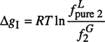
The fugacity of the hypothetical pure liquid has been correlated in a corresponding-states plot shown in Fig. 10-13; the fugacity of the solute, divided by its critical pressure, is shown as a function of the ratio of the solution temperature to the solute’s critical temperature. The fugacities in Fig. 10-13 are for a total pressure of 1.013 bar. If the solution under consideration is at a considerably higher pressure, the Poynting correction should be applied to the fugacity as read from Fig. 10-13; thus

(10-41)

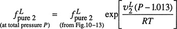
Figure 10-13 Fugacity of hypothetical liquid at 1.013 bar.

where P is in bar.

Equation (10-39) contains Φ₁ the volume fraction of the solvent and, therefore, solving for x₂ requires a trial-and-error calculation; however, the calculation converges rapidly. If the partial pressure of the gas is not large, x₂ is usually very small, and thus setting Φ₁ equal to unity in Eq. (10-39) provides an excellent first approximation.

Shair’s technique for correlating gas solubilities with regular-solution theory can readily be extended to mixed solvents. To estimate the solubility of a gas in a mixture of two or more solvents, Eq. (10-39) should be replaced by

(10-42)

where is an average solubility parameter for the entire solution:

The summation in the definition above is over all components, including the solute.

Table 10-7 and Fig. 10-13 do not include information for the light gases, helium, hydrogen, and neon. For these gases, Hildebrand’s correlations are useful near room temperature and for low temperatures, a separate correlation for hydrogen is available.¹² Good solubility data for hydrogen, helium, and neon are rare at higher temperatures.

¹² see Table 10-4

The correlation given by Eq. (10-39), Table 10-7, and Fig. 10-13 gives fair estimates of gas solubilities over a moderate temperature range for nonpolar gases and liquids. It is not to be expected that this simple correlation should give highly accurate results but, in view of the poor accuracy of many of the experimental solubility data reported in the literature, the estimated solubilities may, in some cases, be more reliable than the experimental ones. Whenever really good experimental data are available, they should be given priority, but whenever there is serious disagreement between observed results and those calculated from a pertinent correlation, one must not, without further study, immediately give preference to the experimental value.

Gas solubilities can also be calculated from an equation of state using the methods discussed in Chaps. 3 and 12. The essential requirement is that the equation of state must be valid for the solute-solvent mixture from zero density to the density of the liquid. The equation of state gives fugacity coefficients; Henry’s constant for solute 2 in solvent 1 is given by

(10-43)

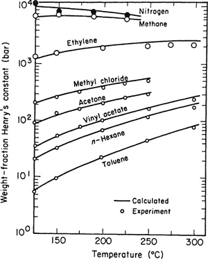
where is the fugacity coefficient of the solute in the liquid solvent at infinite dilution. For example, Plocker et al. (1978) calculated Henry’s constants for hydrogen in hydrocarbons using Lee and Kesler’s form of the Benedict-Webb-Rubin equation (see Sec. 4.14) with results¹³ shown in Fig. 10-14. Another example is provided by Liu (1979), who calculated Henry’s constants for a variety of solutes in low-density polyethylene using an equation of state based on perturbed-hard-chain theory (see Sec. 12.10); Liu’s results are shown in Fig. 10-15. Calculations for Henry’s constants based on an equation of state inevitably require at least one adjustable binary parameter.

¹³ Similar calculations can be made using the corresponding-states tables of Lee and Kesler (see Chap. 4) as shown by Yorizane and Miyano, 1978, AIChEJ., 24: 181.

Figure 10-14 Henry’s constants for hydrogen calculated from the Lee-Kesler extension of the Benedict-Webb-Rubin equation of state. Each binary system requires one adjustable binary parameter. Experimental data from Cukor (1972).

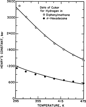
Figure 10-15 Henry’s constants in polyethylene calculated from the perturbed-hard chain equation of state. Each binary system requires one adjustable parameter. Here Henry’s constant is defined as the ratio of fugacity to weight fraction of the solute in the approaches zero.

Gas Solubilities from Scaled-Particle Theory. A statistical-mechanical theory of dense fluids developed by Reiss and coworkers (1960) yields an approximate expression for the reversible work required to introduce a spherical particle of species 2 into a dense fluid containing spherical particles of species 1. This theory, called scaled particle theory, serves as a convenient point of departure for correlating gas solubilities, as shown, for example, by Pierotti (1976), Wilhelm and Battino (1971), and Gel-Isretal. (1976).

Consider a very dilute solution of nonpolar solute 2 in nonpolar solvent 1 at low pressure and at a temperature well below the critical of the solvent. Henry’s constant is given by

(10-44)

where ν₁ is the molar volume of the solvent. Equation (10-44) assumes that the dissolution process can be broken into two steps: in the first step, a cavity is made in the solvent to allow introduction of a solute molecule; in the second step, the solute molecule interacts with surrounding solvent. For the solute, the partial molar Gibbs energies _c and _i stand, respectively, for the first step (cavity formation) and for the second step (interaction).

Let a₁ be the hard-sphere diameter for solvent and a₂ that for solute. If the total pressure is low, scaled-particle theory gives for g_c,

(10-45)

where (N_A is Avogadro’s constant)

(10-45a)

To obtain an expression for _i we assume first that there are no entropic contributions to the interaction; in other words, we assume that all changes in entropy that result from dissolution of a gas in a solvent are given by the cavity-formation calculation. Second, we assume some potential function for describing solute-solvent intermolecular forces. When the Lennard- Jones- 12,6 potential is used, Wilhelm and Battino obtain

(10-46)

where σ₁₂ and ε₁₂ are parameters in the Lennard- Jones potential, k is Boltzmann’s constant and R is the universal gas constant.

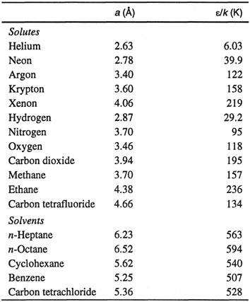
Equations (10-44), (10-45), and (10-46) provide the basis for a correlation of gas solubilities in simple nonpolar systems. Within the approximations used here, it is reasonable to set σ₁₂= l/2(a₁+a₂). The adjustable parameters, then, are a₁, a₂, and ε₁₂/k. Making the further (drastic) simplification ε₁₂= (ε₁ε₂)^1/2, Wilhelrn and Battino correlate solubilities in terms of pure-component parameters only, as shown in Table 10-8. In this correlation, the parameters for the solutes were determined independently (primarily from second-virial-coefficient data) and those for the solvents were adjusted to give the best fit for the gas-solubility data at 25°C. The adjustable parameters are in reasonable agreement with those obtained from other physical properties.

Table 10-8 Correlating parameters for gas solubilities in nonpolar systems at 25°C using scaled-particle theory (Wiihelm and Battino, 1971).

It is possible to extend the scaled-particle method to systems containing polar solutes by adding an induction term to Eq. (10-46), as shown by Wilhelm and Battino (1971) and Geller et al. (1976). Extension to aqueous systems is discussed by Pierroti (1976).

Scaled-particle theory is a particular form of perturbation theory, i.e., a theory that uses theoretical results for hard-sphere systems (no attractive forces) as a point of departure. Application of perturbation theory to gas solubilities is discussed, for example, by Gubbins and coworkers (Shoor, 1969; Tiepel, 1973), Masterson et al. (1969), and Boublik and Lu (1978).

Scaled-particle theory, and most similar perturbation theories, assume that all molecules are rigid, and that the so-called “internal” molecular degrees of freedom (rotation and vibration) are not changed by the dissolution process. This assumption is reasonable only for small spherical molecules. For nonspherical molecules it is likely that, contrary to assumption, solute-solvent interaction forces contribute to the entropy.

When correlating solubility data, failure to take into account changes in the “internal” degrees of freedom is often not important when attention is confined to solubilities at one temperature because the errors are absorbed in the adjustable parameters. However, when solubilities are to be correlated for an appreciable range of temperature, neglecting the entropy of interaction [as was done in deriving Eq. (10-46)] may produce a temperature dependence for adjustable parameters r and ε2. An example of such a correlation is provided by Schulze (1981), who used scaled-particle theory to correlate solubilities of simple gases in water from 0 to (about) 300°C.

10.6 Gas Solubility in Mixed Solvents

Good solubility data for gases in pure liquids are not plentiful, while solubility data in mixed solvents are scarce. With the aid of a simple molecular-thermodynamic model, however, it is often possible to make a fair estimate of the solubility of a gas in a simple solvent mixture, provided that the solubility of the gas is known in each of the pure solvents that comprise the mixture. The procedure for making such an estimate is, essentially, based on Wohl’s expansion (Secs. 6.10 and 6.14), as discussed by O’Connell (1964).

Let subscript 2 stand for the gas as before, and let subscripts 1 and 3 stand for the two (miscible) solvents. To simplify matters, we confine attention to low or moderate pressures where the effect of pressure on liquid-phase properties can be neglected. For the ternary liquid phase, we write the simplest (two-suffix Margules) expansion of Wohl for the excess Gibbs energy at constant temperature

(10-47)

where each a_ij is a constant characteristic of the ij binary pair.

From Eq. (10-47) we can compute the symmetrically normalized activity coefficient γ₂ of the gaseous solute using Eq. (6-25). The unsymmetrically normalized activity coefficient can then be found by

(10-48)

where the definition of is

(10-49)

As in previous sections, H_2,1 i stands for Henry’s constant of component 2 in solvent 1 at system temperature. O’Connell also has shown that for this simple model, parameters a₂₃ and; a₁₂ are related to the two Henry’s constants:

(10-50)

where H_2,3 is Henry’s constant for the solute in solvent 3 at system temperature.

From Eqs. (10-47) and (10-48), utilizing Eq. (6-25), we obtain

(10-51)

We now use Eqs. (10-50) and (10-50) to obtain an expression for H_2,mixture, Henry’s constant for the solute in the mixed solvent. For some fixed ratio of solvents 1 and 3,

(10-52)

From Eq. (10-51),

(10-53)

Substitution of Eqs. (10-50) and (10-50) into Eq. (10-52) gives the desired result:

(10-54)

Equation (10-54) says that the logarithm of Henry’s constant in a binary solvent mixture is a linear function of the solvent composition whenever the two solvents (without solute) form an ideal mixture (a₁₃=0). If the solute-free mixture exhibits positive deviations from Raoult’s law (a₁₃>0), Henry’s constant in the mixture is smaller (or solubility is larger) than that corresponding to an ideal mixture of the same composition. Similarly, if a₁₃<0, the solubility of the gas is lower than what it would be if the solvents formed an ideal mixture. Constant a₁₃ must be estimated from vapor-liquid equilibrium data for the solvent mixture.¹⁴

¹⁴ For nonpolar solvents an estimate can sometimes be made using the theory of reguiar solutions:

where δ is the solubility parameter and V^L the liquid molar volume. see Sec. 7.2.

According to Eq. (10-54), the effect of nonideal mixing of the solvents is not large. To illustrate, two calculated examples at 25°C are shown in Fig. 10-16. The first one considers Henry’s constants for hydrogen in mixtures of toluene and heptane. Since toluene and heptane show only modest positive deviations from Raoult’s law (g^E-=1380 mol^-1 for the equimolar mixture), a₁₃ is small and, as shown in Fig. 10-16, Henry’s constant calculated from Eq. (10-54) differs little from that calculated assuming an ideal solvent mixture. The second example considers Henry’s constants for oxygen in mixtures of isooctane and perfluoroheptane, a system that exhibits large deviations from Raoult’s law; for the equimolar mixture of these solvents g^E- 1380 J mol^-1 and at temperatures only slightly below 25°C, these two liquids are no longer completely miscible. In this case there is a more significant difference between Henry’s constants calculated with and without nonideality of the solvent mixture. For an equimolar mixture of the two solvents, the calculated solubility of oxygen is enhanced by nearly 20% as a result of the solvent mixture’s nonideality.

Figure 10-16 Calculated Henry’s constants in solvent mixtures at 25°C.

Equation (10-54) is readily generalized to solvent mixtures containing any desired number of solvents. For an m-component system where the gas is designated by subscript 2, Henry’s constant for the gaseous solute is given by

(10-55)

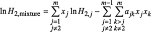
Equation (10-55), like Eq. (10-54), follows directly from the simplest form of Wohl’s expansion as given by Eq. (10-47) for a ternary mixture.

Table 10-9 shows results obtained for the solubility of carbon dioxide in an aqueous solution of diglyme (diethylene glycol dimethyl ether with molar mass of 134.2 g mol^-1

Table 10-9 Parameter a₁₃ of Eq. (10-54) (with volume fractions instead of mole fractions) for the solubility of carbon dioxide in aqueous digiyme at 25°C (Sciamanna and Lynn, 1988). Henry’s constants in bar. Values of H_2,mixture for ideal solutions were obtained from Eq. (10-54) (with mole fractions replaced by volume fractions) and with a₁₃ = 0. When the indicated values of a₁₃ are used, calculated Henry’s constants are identical to those obtained from experiment.

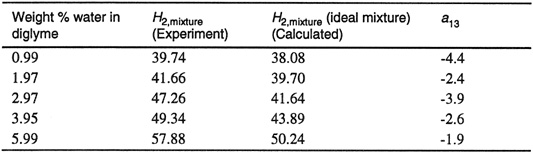
The negative values for a₁₃ indicate that the water-solvent mixture exhibits negative deviations from Raoult’s law, probably due to hydrogen bonding between water and solvent molecules. However, for the particular case shown in Table 10-9, the ideal-solution mixing rule [Eq. (10-54) with a₁₃ = 0] is adequate as a first approximation.

In these calculations, the important assumption is that Eq. (10-47) (or a similar relation using volume fractions) gives a valid description of the excess Gibbs energy of the ternary mixture. This assumption provides a reasonable approximation for some solutions of simple fluids, but for mixtures containing polar or hydrogen-bonded liquids a better model is required. For such cases, binary data may not be sufficient; a ternary constant may be necessary.

Nitta et al. (1973) have also used Wohl’s expansion to obtain an expression for the solubility of a gas in a mixed solvent. As shown below, this expression takes into account the effect of self-association of one of the solvents.

We define a residual quantity by

(10-56)

where H_i,mixture is Henry’s constant for solute i in the solvent mixture containing m solvents; H_i,j is Henry’s constant for solute i in solvent j and Φ_j is the volume fraction of solvent j in the solvent mixture on a solute-free basis.¹⁵

¹⁵ It is sometimes customary to define an excess Henry’s constant

where x is the mole fraction.

If the solvents form an ideal mixture over the entire range of solvent compositions, in = 0. In a binary mixture containing solvents a and b, the residual quantity is related to by

where r is the ratio of liquid molar volumes v_b/v_a. We see that In vanishes only when both ()_size and ()_{physical interaction} go to zero.

We can obtain an expression for using Wohl’s expansion for the excess Gibbs energy; for all binary pairs i-j, i-k, j-k,…, we assume the Flory-Huggins equation. Omitting algebraic details, we obtain

(10-57)

where

(10-58)

(10-59)

where v, the molar volume of the solute-free solvent mixture, is given by,

(10-60)

with x denoting the mole fraction. In Eq. (10-59), v_i is the molar “liquid” volume of solute i and x_jk is a Flory interaction parameter for solvents j and k, here expressed in units of energy per unit volume.

If one of the solvents (say, solvent k) is an alcohol (or amine) that associates continuously, then an additional term appears in Eq. (10-57):

(10-61)

The association term is given by

(10-62)

where the association constant for solvent k is defined by

(10-63)

Here, c₁ stands for the concentration (moles per unit volume) of monomer and c_n for the concentration of polymer of degree n.

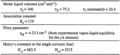
To illustrate this discussion of gas solubility in a mixed solvent, Nitta et al. (1973) reduced experimental solubility data for nitrogen in the mixed solvent isooctane (j)/n-propanol (k) at 25°C. Parameters are given in Table 10-10 and results are shown in Fig. 10-17.

Table 10-10 Parameters for calculating Henry’s constant for nitrogen (/) in the mixed solvent system isooctane (/)/n-propanol (k) at 25°C (Nitta et al., 1973).

For positive x_jk, the physical interaction contribution to is negative; the association contribution is also negative. These contributions, therefore, tend to increase gas solubility. However, the size contribution is positive, tending to lower gas solubility.

As indicated in Fig. 10-17, agreement between calculated and observed Henry’s constants is remarkable, considering that only binary and single-component data were used in the calculation. In this example, if Henry’s constants had been calculated assuming that a plot of ln H_i,mixture versus x_k is a straight line, the calculated Henry’s constants at x_k = 0.5 would be about 30% too large. In this case that error is not as large as it might be because of partial cancellation in Eq. (10-61), where the first term on the left is positive while the other two are negative.

Figure 10-17 Solubility of nitrogen in a mixed solvent containing isooctane and n-propanol at 25°C. See Eq. (10-56).

In general it is not possible, without strong simplifying assumptions, to calculate the solubility of a gas in a mixed solvent using only binary data. A more rigorous discussion, based on the direct correlation function of liquids, has been presented by O’Connell (1971) and an extension of perturbation theory to multisolvent systems has been presented by Tiepel and Gubbins (1973).

10.7 Chemical Effects on Gas Solubility

The gas-solubility correlations of Hildebrand and Scott and of Shair, discussed in Sec. 10.5, are based on a consideration of physical forces between solute and solvent; they are not useful for those cases where chemical forces are significant. Sometimes these chemical effects are not large and therefore a physical theory is a good approximation. But frequently chemical forces are dominant; in that case, correlations cannot easily be established because specific chemical forces are not subject to simple generalizations. An extreme example of a chemical effect in a gas-liquid solution is provided by the interaction between sulfur trioxide and water (to form sulfuric acid); somewhat milder examples are the interaction between acetylene and acetone (hydrogen bonding) or that between ethylene and an aqueous solution of silver nitrate (Lewis acid-base complex formation); a still weaker case of the effect of chemical forces was mentioned earlier in connection with Fig. 10-11, where the solubility of (acidic) carbon dioxide in (basic) benzene and toluene is larger than that predicted by a physical correlation. In each of these cases the solubility of the gas is enhanced as a result of a specific affinity between solute and solvent.

Systematic studies of the effect of chemical forces on gas solubility are rare, primarily because it is difficult to characterize chemical forces in a quantitative way; the chemical affinity of a solvent (unlike its solubility parameter) depends on the nature of the solute, and therefore a measure of chemical effects in solution is necessarily relative rather than absolute.¹⁶ A few examples, given below, illustrate how the effect of chemical forces on gas solubility can be studied in at least a semiquantitative way.

¹⁶ As shown later, a potentially useful method for characterizing specific solute-solvent interactions is provided by donor-acceptor numbers. See, for example, Viktor Gutmann, 1978, The Donor-Acceptor Approach to Molecular Interactions, New York: Plenum Press.

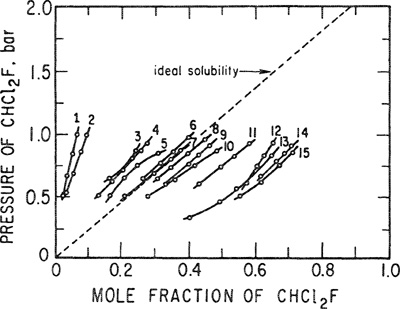
The importance of chemical effects is shown by the solubilities of dichlorofluoromethane (Freon-21) at 32.2°C in a variety of solvents. Solubility data in 15 solvents, obtained by Zellhoefer et al. (1938) are shown in Fig. 10-18 as a function of pressure. Because the critical temperature of Freon-21 (178.5°C) is well above 32.2°C, it is possible to calculate an ideal solubility [Eq. (10-2)] without extrapolation of the vapor-pressure data; this ideal solubility is shown in Fig. 10-18 by a dashed line. Figure 10-18 indicates that the solvents fall roughly into three groups: In the first group, the solubility is less than ideal (positive deviations from Raoult’s law); in the second group, deviations from Raoult’s law are very small; and in the third group, the solubility is larger than ideal (negative deviations from Raoult’s law). These data can be explained qualitatively by the concept of hydrogen bonding; Freon-21 has an active hydrogen atom and whenever the solvent can act as a proton acceptor, it is a relatively good solvent. The stronger the proton affinity (Brönsted basicity) of the solvent, the better that solvent is, provided that the proton-accepting atom of the solvent molecule is not already “taken” by a proton from a neighboring solvent molecule. In other words, if the solvent molecules are strongly self-associated, they will not be available to form hydrogen bonds with the solute. As a result, strongly associated substances are poor solvents for solutes such as Freon-21 that can form only weak hydrogen bonds and thus cannot compete successfully for proton acceptors. It is for this reason that the glycols are poor solvents for Freon-21; while no data for alcohols are given in Fig. 10-18, it is likely that methanol and ethanol would also be poor solvents for Freon 21.

Figure 10-18 Solubility of Freon-21 in liquid solvents at 32.2°C. Solvents are: 1. Ethylene giycoi; 2. Trimethylene giycol; 3. Decaiin; 4. Aniline; 5. Benzotrifluoride; 6. Nitrobenzene; 7. Tetralin; 8. Bis-p methyithioethy! sulfide; 9. Dimethylaniline; 10. Dioxan; 11. Diethyl oxaiate; 12. Diethyl acetate; 13. TetrahydrofurfuryS iaurate; 14. Tetraethy! oxamide; 15. Dimethyl ether of tetraethylene giycol.

Aromatic solvents aniline, benzotrifluoride, and nitrobenzene are weak proton acceptors and it appears that for these solvents, chemical forces (causing negative deviations from Raoult’s law) are just strong enough to overcome physical forces (that usually cause positive deviations from Raoult’s law), with the result that the observed solubilities are close to ideal. Finally, those solvents that are powerful proton acceptors – and whose molecules are free to accept protons – are excellent solvents for Freon-21. Dimethylaniline, for example, is a much stronger base and hence a better solvent than aniline. The oxygen atoms in ethers and the nitrogen atoms in amides are also good proton acceptors for solute molecules because ethers and amides do not self-associate to an appreciable extent.

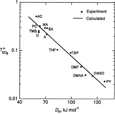
Figure 10-19 presents a correlation that provides Henry’s constants in terms of “chemical” thermodynamic parameters.¹⁷ This figure shows an empirical correlation of a macroscopic thermodynamic property (infinite-dilution activity coefficients for sulfur dioxide in organic solvents) with specific solvent molecular characteristics (the Gutmann donor¹⁸ number, a basicity scale). As discussed earlier, Henry’s constant is directly related to the activity coefficient at infinite dilution; see Eq, (6-43). In this case, Henry’s constant is the product of and the vapor pressure of pure SO₂ liquid at 25°C.

Figure 10-19 Correlation of infinite-dilution activity coefficients of SO₂ with solvent Gutmann donor number at 25°C. The solvents shown are: A - Acetone; AC - Acetonitrile; D - 1,4-Dioxane; DMAA - N,N-Dimethylacetamide; DMF - N,N-Dimethylformamide; DMSO - Dimethyl sulfoxide; EA - Ethyl acetate; MA - Methyl acetate; PC - Propylene carbonate; PY- Pyridine; TBP - Tributy! phosphate; THF - Tetrahydrofuran; TMS - Tetramethylene suifone. ——Calculated from Eq. (10-64); • Experiment.

¹⁷ R. J. Demyanovich and S. Lynn, 1991, J. Sol. Chem., 20: 693.

¹⁸ We follow here the Lewis definition of acids (electron-pair acceptors) and bases (electron-pair donors) to distinguish between acceptors and donors.

To characterize the electron-donor ability of a molecule, Gutinann defines the donor number D_N (or donicity) as the molar enthalpy value (-Δh) for the reaction of the donor (D) with SbCl₅ as a reference acceptor in a 10^-3 M solution of SbCl₅ in dichioroethane:

The molar enthalpy of the 1:1 adduct formed is taken as an approximate measure of the energy of the coordinate bond between donor and acceptor. However, the stability of the adduct is a function of Δg⁰, the Gibbs energy of adduct formation. If a linear relation exists between Δg⁰ and -Δh, then the enthalpy values (or donor numbers) can be used as a guide to the relative complex stabilities. Gutmann observed a linear relation between -Δh and In K for the adduct formed by SbCl₅ and various donors; here K is the equilibrium constant for adduct formation, related to Δg⁰ by –RT ln K = Δg⁰. Table 10.11 lists the donor numbers for several solvents obtained from calorimetric measurements.

Table 10-11 Donor numbers (D_N) for several solvents obtained from calorimetric measurements in 10^-3 M solutions of SbCl₅ in dichloroethane (SbCl₅ is the reference acceptor).

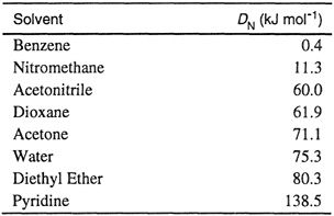
As Fig. 10.19 shows, in the region 60 ≤ D_N ≤ 150 kJ mol^-1, there is a linear relation between the logarithm of the activity coefficient of SO₂ at infinite dilution and the Gutmann donor number (in kJ mol^-1):

(10-64)

Using this linear relation, it is possible to estimate Henry’s constants for sulfur dioxide in a variety of “chemical” organic solvents.

While the chemical characteristics of solvents can be used to correlate gas solubilities, it is also possible to use gas-solubility data to characterize solvents as illustrated by solubility data for hydrogen chloride gas in heptane solutions of aromatic hydrocarbons at a low temperature. The solubility data of Brown and Brady (1952) are shown in Fig. 10-20. Because the pressure of hydrogen chloride gas was kept very low, Henry’s law holds; Henry’s constants (the slopes of the lines in Fig. 10-20) are shown in Table 10-12.

Figure 10-20 Solubility of hydrogen chloride at -78.51°C in n-heptane and in 5 mol % solutions of aromatics in n-heptane.

Table 10-12 Henry’s constants for solubility of HCl in 5 mol % solutions of aromatics in n-heptane, and dissociation constants K for complex formation (all at -78.51°C).

The solubility data show that addition of small amounts of aromatics to heptane increases the solubility of hydrogen chloride. This increase is a result of the electron-donating properties of aromatic molecules that, because of their π-electrons, can act as Lewis bases. The solubility data, therefore, can be explained by postulating the formation of a complex between hydrogen chloride and aromatics; the stability of the complex depends on the ability of the aromatic to donate electrons and this, in turn, is determined by the nature of the substituent on the benzene ring. Halide groups such as CF3 and Cl withdraw electrons and decrease the electron density on the benzene ring, while methyl groups donate electrons and increase the electron density on the ring. Therefore, relative to benzene, toluene is a stronger Lewis base while chlorobenzene is weaker.

The abilities of substituents on benzene to donate or withdraw electrons have also been determined from theoretical calculations, from ionization potentials, and from chemical-kinetic data (Hine, 1962; Hamrnett, 1970); the results are in excellent agreement with those obtained from solubility studies. Further evidence that hydrogen chloride and aromatics form stable complexes at low temperatures is given by the freezing-point data of Cook et al. (1956) for mixtures of hydrogen chloride and mesitylene shown in Fig. 10-21. The maximum at a mole fraction of one-half shows that the stoichiometric ratio of hydrogen chloride to aromatic in the complex is 1:1.

Figure 10-21 Evidence for complex formation: freezing points for hydrochloric acid/mesitylene mixtures.

Brown and Brady reduced their solubility data by calculating dissociation equilibrium constants for the complexes; the dissociation constant is defined by

(10-65)

where x stands for mole fraction and p for partial pressure. According to this definition, the stability of a complex falls as the dissociation constant rises. By simple stoichiometry and by assuming that the complex is nonvolatile, Brown and Brady were able to calculate K from the change in Henry’s constant in heptane that results when aromatic molecules are added to the solvent. Their results are shown in Table 10-12. The aromatic components are listed in order of rising basicity. As basicity increases, the solubility also increases and Henry’s constant falls. Although the concentration of the aromatic solvent is only 5 mol % in an excess of “inert” heptane, the effect of the aromatic component on the solubility of HCl is pronounced; the presence of 5 mol % mesitylene almost doubles the solubility.

In the preceding paragraphs, we showed the effect of chemical forces on Henry’s constant. In the final example, we show how chemical forces can account for deviations from Henry’s law; as an illustration we consider the solubility of a gas that dissociates in solution.

Deviations from Henry’s law may result from chemical effects even at very low solute concentrations. In Secs. 10.2 and 10.3 we discussed how departures from Henry’s law may be due to advanced pressures, to large dissimilarity between solvent and solute, or both. However, whenever the gaseous solute experiences a chemical change such as association or dissociation in the solvent, Henry’s law fails because the equilibrium between the vapor phase and the liquid phase is then coupled with an additional (chemical) equilibrium in the liquid phase. We briefly discuss such a case here by analyzing data for the solubility of sulfur dioxide in water at 25°C, shown in Table 10-13.

Table 10-13 Solubility of sulfur dioxide in water at 25°C.*

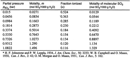
The first column in Table 10-13 gives the partial pressure of sulfur dioxide that in this case Is essentially equal to the fugacity. The second column gives the molality of sulfur dioxide in aqueous solution that at these very low concentrations is proportional to the solute mole fraction. However, when plotted, these data do not yield a straight line; despite the very low concentrations of sulfur dioxide, Henry’s law is not valid.

The reason for the failure of Henry’s law becomes apparent when we consider that sulfur dioxide plus water produces hydrogen ions and bisulfite ions. When sulfur dioxide gas is in contact with liquid water, we must consider two equilibria:

Henry’s law governs only the (vertical) equilibrium between the two phases; in this case, Henry’s law must be written

(10-66)

where p is the partial pressure of sulfur dioxide, H is a “true” Henry’s constant, and m_M is the molality of molecular (nonionized) sulfur dioxide in aqueous solution.

Johnstone and Leppia (1934) have calculated α, the fractional ionization of sulfur dioxide in water, from electrical conductivity measurements; these are given in the third column of Table 10-13. The fourth column gives m_M given by the product of m, the total molality, and (1 – α). When the partial pressure of sulfur dioxide is plotted against m_M (rather than m), a straight line is obtained.

This case is particularly fortunate because independent conductivity measurements are available and thus it was easily possible quantitatively to reconcile the solubility data with Henry’s law. In a more typical case, independent data on the liquid solution (other than the solubility data themselves) would not be available; however, even then it is possible to linearize the solubility data by construction of a simple but reasonable model, similar to that given in Sec. 7.14.

For equilibrium between sulfur dioxide in the gas phase and molecular sulfur dioxide in the liquid phase we write

(10-67)

For ionization equilibrium in the liquid phase we write

(10-68)

where K is the ionization equilibrium constant. Substituting Eq. (10-67), we have

(10-69)

from which we obtain α:

(10-70)

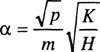
Further substitution and rearrangement finally gives

(10-71)

Equation (10-71) shows the effect of ionization on Henry’s law; if there were no ionization, K = 0 and Henry’s law is recovered. The ability of a solute to ionize in solution increases its solubility; however, as the concentration of solute in the solvent rises, the fraction ionized falls. Therefore, the “effective” Henry’s constant p/m rises with increasing pressure and a plot of p versus m is not linear but convex toward the horizontal axis.

Figure 10-22 presents solubility data for the sulfur dioxide/water system plotted according to Eq. (10-71). A straight line is obtained. A plot such as this is useful for smoothing, interpolating and cautiously extrapolating limited gas-solubility data for any system where the gaseous solute tends to ionize (or dissociate) in the solvent.

Figure 10-22 Effect of ionization on solubility. Linearization of solubility data for sulfur dioxide in water at 25°C.

The effect of ionization on solubility is particularly strong when two volatile, ionizing solutes, one basic and one acidic, are dissolved in an ionizing (high-dielectricconstant) solvent such as water (Edwards et al., 1978; Beutier and Renon, 1978a). To illustrate, consider an aqueous solution containing two volatile weak electrolytes: acidic carbon dioxide and basic ammonia. In this ternary mixture, ionization is more drastic than in either binary aqueous mixture because H⁺ ions (produced by the reaction of carbon dioxide with water) interact with OH^– ions (produced by the interaction of ammonia with water). Since water has only a small tendency to ionize, the equilibrium

lies far to the right. As a result, the presence of carbon dioxide enhances the solubility of ammonia, and vice versa. This enhancement is shown in Fig. 10-23 that presents calculated partial pressures for the two weak volatile electrolytes in water as a function of carbon dioxide/ammonia ratio at 100°C when the total ammonia concentration is 6.75 molal. The indicated values of K are ionization equilibrium constants for the reactions

Figure 10-23 Enhancement of solubilities due to chemical interactions. The system carbon dioxide/ammonia/water contains 6.75 molal ammonia at 100°C.

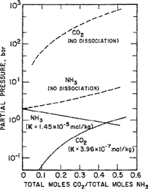
and

The continuous lines take chemical equilibria into account but the dashed lines do not. Because the ordinate is logarithmic, failure to consider chemical equilibria yields partial pressures that are much too large.

These examples illustrate how chemical effects may have a large influence on solubility behavior. It must be remembered that a solvent is never an inert material that merely acts as a cage for the solute, although it is frequently tempting to think of it that way. Solvent and solute always interact and, historically, when the interaction is strong enough to result in a new species, we call it chemical. But, as discussed in Sees. 7.9 to 7.14, this is only a convenience, useful for classification. There is no sharp boundary between physical and chemical forces; all molecules have forces acting between them and it is these forces that determine solubility regardless of whether they fall into a physical or chemical classification. For interpreting solubility behavior, however, it is often worthwhile to utilize these classifications by first taking into account the more easily generalized physical forces and then correcting for specific chemical effects. This is essentially what Brown and Brady did since they assumed that the physical forces between hydrogen chloride and hydrocarbons are the same regardless of the nature of the hydrocarbon and that any excess solubility is due to chemical-complex formation. Such a procedure is both simple and practical but its molecular significance must not be taken too seriously unless there is additional, independent evidence for the existence of a complex.

Similarly, the solubility behavior of sulfur dioxide in water can be explained in terms of a physical Henry’s law coupled with a chemical equilibrium for a dissociation reaction whose existence is supported by physicochemical data other than the solubility data themselves.

A thorough review of gas solubility is given by Fogg and Gerard (1991). This review clearly shows that despite its obvious importance in biology, medicine, and chemical engineering, our fundamental understanding of gas-liquid equilibria is still in a rudimentary stage. Fogg and Gerrard present a comprehensive description of the experimental methods for measuring gas solubilities. They also discuss factors influencing gas solubility, and present gas-solubility data for various industrial gases.

References

Alvarez, J., H. R. Corti, R. Femández-Prini, and M. L. Japas, 1994, Geochim. Cosmochim. Ada, 58: 2789.

Bender, E., U. Klein, W. Schmitt, and J. M. Prausnitz, 1984, Fluid Phase Equilibria, 15: 24.

Benson, B. B. and D. Krause, Jr., 1976, J. Chem. Phys., 64: 689.

Beutier, D. and H. Renon, 1978, AIChE J., 24: 1122.

Beutier, D. and H. Renon, 1978a, Ind. Eng. Chem. Process Des, Dev., 17: 220.

Boublik, T. and B. C.-Y. Lu, 1978, J. Phys. Chem., 82: 2801.

Brown, H. C. and J. O. Brady, 1952, J. Am. Chem. Soc., 74: 3570.

Brunner, E., 1978, Ber. Bunsenges. Phys. Chem., 82: 798.

Brunner, E., 1979, Ber. Bunsenges. Phys. Chem., 83: 715.

Cook, D., Y. Lupien, and W. G. Schneider, 1956, Can. J. Chem., 34: 964.

Cukor, P. M. and J. M. Prausnitz, 1972, J. Phys. Chem., 76: 598.

Dodge, B. F. and R. H. Newton, 1937, Ind. Eng. Chem., 29: 718.

Edwards, T. J., G. Maurer, J. Newman, and J. M. Prausnitz, 1978, AIChE J., 24: 966.

Fogg, G.T. and W. Gerrard, 1991, Solubility of Gases in Liquids. Chichester: John Wiley & Sons, 1991. See also Clever and Battino, 1975, Solutions and Solubilities, Part 1 (M. R. J. Back, Ed.), Techniques of Chemistry, Vol.VIII, New York: Wiley-Interscience; W. Gerrard, 1976, Solubility of Gases and Liquids, New York: Plenum Press; and W. Gerrard, 1980, Gas Solubilities, Oxford: Pergamon Press; IUPAC Solubility Data Series, beginning in 1979, Oxford: Pergamon Press.

Geller, E. B., R. Battino, and E. Wilhelm, 1976, J. Chem. Thermodynamics, 8:197.

Hammett, L. P., 1970, Physical Organic Chemistry, 2^nd Ed. New York: McGraw-Hill.

Harvey, A. H. and J. M. H. Levelt Sengers, 1990, AIChE J., 36: 539.

Harvey, A. H., 1996, AIChE J., 42: 1491.

Hildebrand, J. H. and R. L. Scott, 1962, Regular Solutions. Englewood Cliffs: Prentice-Hall.

Hine, J., 1962, Physical Organic Chemistry, 2^nd Ed. New York: McGraw-Hill.

Hirschfelder, J. O., C. F. Curtiss, and R. B. Bird, 1954, Molecular Theory of Gases and Liquids. New York: John Wiley & Sons.

Japas, M. L. and J. M. H. Levelt Sengers, 1989, AIChE J., 35: 705.

Johnstons, H. F. and P. W. Leppla, 1934, J. Am. Chem. Soc., 56: 2233.

King, M. B., K. Kassim, andH. Al-Najjar, 1977, Chem. Eng. Sci., 32: 1247.

Krichevsky, I. R. and J. S. Kasamovsky, 1935, J. Am. Chem. Soc., 57: 2168.

Krichevsky, I. R. and A. A. Ilinskaya, 1945, Zh. Fit. Khim. USSR, 19: 621.

Levelt Sengers, J. M. H., 1991, Supercritical Fluid Technology: Reviews in Modern Theory and Applications, Chap. 1, (T. J. Bruno and J. F. Ely, Eds.). Boca Raton: CRC Press.

Liu, D. D. and J. M. Prausnitz, 1979, J. Appl. Poly. Sci., 24: 725.

Masterson, W. L., T. P. Lee, and R. L. Boyington, 1969, J. Phys. Chem., 73: 2761.

Nitta, T., A. Tatsuishi, and T. Katayama, 1973, J. Chem. Eng. Jap., 6: 475.

O’Connell, J. P. and J. M. Prausnitz, 1964, Ind. Eng. Chem. Fundam., 3: 347.

O’Connell, J. P., 1971, AIChE J., 17: 658.

Orentlicher, M. and J. M. Prausnitz, 1964, Chem. Eng. Sci., 19: 775.

Pierotti, R. A., 1976, Chem. Rev., 76: 717.

Plöcker, U., H. Knapp, and J. M. Prausnitz, 1978, Ind. Eng. Chem. Process Des. Dev., 17: 324.

Prausnitz, J. M. and F. H. Shair, 1961, AIChE J., 7: 682.

Reiss, H., H. L. Frisch, E. Helfand, and J. L. Lebowitz, 1960, J. Chem. Phys., 32: 119; ibid., 33: 1379.

Schulze, G. and J. M. Prausnitz, 1981, Ind. Eng, Chem. Fundam., 20: 175.

Sciamanna, S.F. and S. Lynn, 1988, Ind. Eng. Chem. Res., 27: 492.

Sherwood, A. E. and J. M. Prausnitz, 1962, AIChE J., 8: 519; Errata, 1963, ibid., 9: 246.

Shoor, S. K. and K. E. Gubbins, 1969, J. Phys. Chem., 73: 408.

Tiepel, E. W. and K. E. Gubbins, 1973, Ind. Eng. Chem. Fundam., 12: 18.

Wiebe, R. and V. L. Gaddy, 1937, J. Am. Chem. Soc., 59: 1984.

Wilhelm, E. and R. Battino, 1971, J. Chem. Thermodynamics, 3: 379.

Yau, J.-S., and F.-N. Tsai, 1992, J. Chem. Eng. Data, 37, 141; ibid., 1992, Fluid Phase Equilibria, 73: 1.

Yen, L. and J. J. McKetta, 1962, AIChE J., 8: 501.

Zellhoefer, G. F., M. J. Copley, and C. S. Marvel, 1938, J. Am. Chem. Soc., 60: 1337.

Problems

1. Compute the K factor for methane at 13.8 bar and 366 K in a hydrocarbon mixture whose composition in mole percent is 20% benzene, 60% m-xylene, and 20% n-hexane. Use Shair’s correlation.

2. At 20°C, the solubility of helium in argyle acetate is x₂ = 1.00×10^-4 at 25 bar and is x₂ = 2.86×10^-4 at 75 bar. Estimate the solubility of helium in this solvent at 20°C and 150 bar. State all assumptions made.

3. Estimate the solubility of hydrogen gas (at 1 bar partial pressure) in liquid air at 90 K. The following experimental information is available, all at 90 K: x_H2 (1 bar partial pressure) in liquid methane is 0.0549×10^-2; x_H2 (1 bar partial pressure) in liquid carbon monoxide is 0.263×10^-2, Pure-component data (at 90 K):

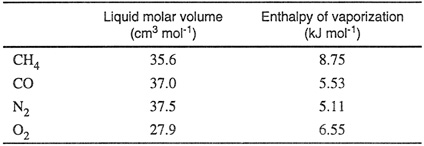
4. The Bunsen coefficient is an experimentally obtainable measure of the solubility of a sparingly soluble gas in a liquid solvent. It is defined as the cubic centimeters of gas, measured at 0°C and 1 atm, that can dissolve in 1 cm³ of liquid, if the partial pressure of the gas above the liquid is 1 atm. Due to its biological importance, the solubility of oxygen in water has been extensively investigated. The following empirical equation gives the Bunsen coefficient (α) of oxygen in water as a function of temperature t(°C):

(a) From the above equation, find Henry’s constant for O₂ in an aqueous system at 1 atm and 20°C.

(b) Find the solubility (in mg dm^-3 or in ppm) of atmospheric oxygen in water at 20°C.

Density of water at 20°C and 1 atm: 0.9982 g cm^-3.
Vapor pressure of water at 20°C: 17.5 mmHg.
Dry air can be taken as 20.95% by volume of oxygen.

5. At 25°C a closed vessel of 3 liter volume contains 180 grams of water, 420 grams of cyclohexane, and 28 grams of nitrogen. Estimate the solubility of nitrogen (mole fraction) in the cyclohexane phase and in the water phase. In this calculation assume that nitrogen behaves as an ideal gas and neglect the mutual solubilities of water and cyclohexane. Data at 25°C:

6. Compute the solubility x₂ of hydrogen in nitrogen at 77 K and 100 bar. At these conditions the vapor-phase fugacity coefficient for pure hydrogen is 0.88 and the saturation pressure of pure liquid nitrogen is i bar. Use Orentlicher’s correlation.

7. Using the gas-solubility correlations of Hildebrand and Scott (not the one of Shair) estimate the solubility of hydrogen in 1-hexene at 0°C when the partial pressure of hydrogen is 2 bar. The solubility parameter of 1-hexene at 25°C is 14.9 (J cm^-3)^1/2.

8. Using experimental and calculated results presented by Olson (Tables 10-2 and 10-3), estimate the solubility of methane in ethylene oxide at 10°C and at a total pressure of 25 bar. State all simplifying assumptions on which your estimate is based.

9. Consider a solution of nitrogen (2) dissolved in n-butane (1) at 250 K. Using the Peng-Robinson equation of state (see Sec. 12.7), calculate:

(a) Henry’s constant H_2,1.

(b) The partial molar volume of nitrogen infinitely dilute in n-butane.

(c) Parameter A of the two-suffix Margules equation.

Data (at 250 K) are as follows:
= 93.035 cm³ mol^-1
= 0.392 bar.
Interaction parameter k₁₂ obtained from VLE data is 0.0867.