Chapter 3
Thermodynamic Properties from Volumetric Data

For any substance, regardless of whether it is pure or a mixture, most thermodynamic properties of interest in phase equilibria can be calculated from thermal and volumetric measurements. For a given phase (solid, liquid, or gas), thermal measurements (heat capacities) give information on how some thermodynamic properties vary with temperature, whereas volumetric measurements give information on how thermodynamic properties vary with pressure or density at constant temperature. Whenever there is a change of phase (e.g., fusion or vaporization), additional thermal and volumetric measurements are required to characterize that change.

Frequently, it is useful to express a selected thermodynamic function of a substance relative to that which the same substance has as an ideal gas at the same temperature and composition and at some specified pressure or density. This relative function is often called a residual function. The fugacity is a relative function because its numerical value is always relative to that of an ideal gas at unit fugacity; in other words, the standard-state fugacity in Eq. (2-38) is arbitrarily set equal to some fixed value, usually 1 bar.¹

¹ Throughout this book we use the pressure unit bar, related to the SI pressure unit (pascal) by 1 bar = 10⁵ pascal = 0.986923 atmosphere.

As indicated in Chap. 2, the thermodynamic function of primary interest is the fugacity that is directly related to the chemical potential; however, the chemical potential is directly related to the Gibbs energy, that, by definition, is found from the enthalpy and entropy. Therefore, a proper discussion of calculation of fugacities from volumetric properties must begin with the question of how enthalpy and entropy, at constant temperature and composition, are related to pressure. On the other hand, as indicated in Chap. 2, the chemical potential may also be expressed in terms of the Helmholtz energy; in that event the first question must be how entropy and energy, at constant temperature and composition, are related to volume. The answers to these questions may readily be found from Maxwell’s relations. We can then obtain exact equations for the thermodynamic functions U, H, S, A, and G; from these we can derive the chemical potential and, finally, the fugacity.

If we consider a homogeneous mixture at some fixed composition, we must specify two additional variables. In practical phase-equilibrium problems, the common additional variables are temperature and pressure, and in Sec. 3.1 we give equations for the thermodynamic properties with T and P as independent variables. However, volumetric data are most commonly expressed by an equation of state that uses temperature and volume as independent variables, and therefore it is a matter of practical importance to have available equations for the thermodynamic properties in terms of T and V; these are given in Sec. 3.4. The equations in Secs. 3.1 and 3.4 contain no simplifying assumptions;² they are exact and are not restricted to the gas phase but, in principle, apply equally to all phases.

² The equations in Secs. 3.1 and 3.4 do, however, assume that surface effects and all body forces due to gravitational, electric, or magnetic fields, etc., can be neglected.

In Sec. 3.3 we discuss the fugacity of a pure liquid or solid, and in Secs. 3.2 and 3.5 we give examples based on the van der Waals equation. Finally, in Sec. 3.6 we consider briefly how the exact equations for the fugacity may, in principle, be used to solve fluid-phase equilibrium problems subject only to the condition that we have available a reliable equation of state, valid for fluid pure substances and their mixtures over a large density range.

3.1 Thermodynamic Properties with Independent Variables P and T

At constant temperature and composition, we can use one of Maxwell’s relations to give the effect of pressure on enthalpy and entropy:

(3-1)

(3-2)

These two relations form the basis of the derivation for the desired equations. We will not present the derivation here; it requires only straightforward integrations clearly given in several publications by Beattie (1942, 1949, 1955). First, expressions for the enthalpy and entropy are found. The other properties are then calculated from the definitions of enthalpy, Helmholtz energy, and Gibbs energy:

(3-3)

(3-4)

(3-5)

(3-6)

(3-7)

The results are given in Eqs. (3-8) to (3-14). It is understood that all integrations are performed at constant temperature and constant composition.

The symbols have the following meanings:

All extensive properties denoted by capital letters (V, U, H, S, A, and G) represent the total property for n_T moles and therefore are not on a molar basis. Extensive properties on a molar basis are denoted by lowercase letters (υ, u, h, s, a, and g). In Eqs. (3-10) to (3-13), pressure P is in bars.

(3-8)

(3-9)

(3-10)

(3-11)

(3-12)

(3-13)

and finally

(3-14)

where is the partial molar volume of i. The dimensionless ratio f_i/y_iP = φ_i is called the fugacity coefficient. For a mixture of ideal gases, φ_i = 1, as shown later.

Equations (3-8) to (3-14) enable us to compute all the desired thermodynamic properties for any substance relative to the ideal-gas state at 1 bar and at the same temperature and composition, provided that we have information on volumetric behavior in the form

(3-15)

To evaluate the integrals in Eqs. (3-8) to (3-14), the volumetric information required in function F must be available not only for pressure P, where the thermodynamic properties are desired, but for the entire pressure range 0 to P.

In Eqs. (3-8) and (3-11), the quantity V appearing in the PV product is the total volume at the system pressure P and at the temperature and composition used throughout. This volume V is found from the equation of state, Eq. (3-15).

For a pure component, and Eq. (3-14) simplifies to

(3-16)

where υ_i is the molar volume of pure i. Equation (3-16) is frequently expressed in the equivalent form

(3-17)

where z, the compressibility factor, is defined by

(3-18)

The fugacity of any component i in a mixture is given by Eq. (3-14) that is not only general and exact but also remarkably simple. One might well wonder, then, why there are any problems at all in calculating fugacities and, subsequently, computing phase-equilibrium relations. The problem is not with Eq. (3-14) but with Eq. (3-15), where we have written the vague symbol F, meaning “some function”. Herein lies the difficulty: What is F? Function F need not be an analytical function; sometimes we have available tabulated volumetric data that may then be differentiated and integrated numerically to yield the desired thermodynamic functions. But this is rarely the case, especially for mixtures. Usually, one must estimate volumetric behavior from limited experimental data. There is, unfortunately, no generally valid equation of state, applicable to a large number of pure substances and their mixtures over a wide range of conditions, including the liquid phase. There are some good equations of state useful for only a limited class of substances and for limited conditions; however, these equations are almost always pressure-explicit rather than volume-explicit. Therefore, it is necessary to express the derived thermodynamic functions in terms of the less convenient independent variables V and T as shown in Sec. 3.4. Before concluding this section, however, let us briefly discuss some of the features of Eq. (3-14).

First, we consider the fugacity of a component i in a mixture of ideal gases. In that case, the equation of state is

(3-19)

and the partial molar volume of i is

(3-20)

Substituting in Eq. (3-14) gives

(3-21)

For a mixture of ideal gases, then, the fugacity of i is equal to its partial pressure, as expected.

Next, let us assume that the gas mixture follows Amagat’s law at all pressures up to the pressure of interest. Amagat’s law states that at fixed temperature and pressure, the volume of the mixture is a linear function of the mole numbers

(3-22)

where υ_i is the molar volume of pure i at the same temperature and pressure and in the same phase.

Another way to state Amagat’s law is to say that at constant temperature and pressure, the components mix isometrically, i.e., with no change in total volume. If there is no volume change, then the partial molar volume of each component must be equal to its molar volume in the pure state. It is this equality which is asserted by Amagat’s law. Differentiating Eq. (3-22), we have

(3-23)

Substitution in Eq. (3-14) yields

(3-24)

Upon comparing Eq. (3-24) with Eq. (3-16), we obtain

(3-25)

Equation (3-25) is the Lewis fugacity rule. In Eq. (3-25), the fugacity of pure i is evaluated at the temperature and pressure of the mixture and for the same phase.

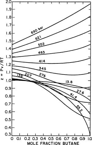
The Lewis fugacity rule is a particularly simple equation and is therefore widely used for evaluating fugacities of components in gas mixtures. However, it is not reliable because it is based on the severe simplification introduced by Amagat’s law. The Lewis fugacity rule is discussed further in Chap. 5; for present purposes it is sufficient to understand clearly how Eq. (3-25) was obtained. The derivation assumes additivity of the volumes of all the components in the mixture at constant temperature and pressure; at high pressures, this is frequently a very good assumption because at liquid-like densities, fluids tend to mix with little or no change in volume. For example, volumetric data for the nitrogen/butane system at 171°C, shown in Fig. 3-1, indicate that at 690 bar the molar volume of the mixture is nearly a straight-line function of the mole fraction (Evans and Watson, 1956). At first glance, therefore, one might be tempted to conclude that for this system, at 690 bar and 171°C the Lewis fugacity rule should give an excellent approximation for the fugacities of the components in the mixture. A second look, however, shows that this conclusion is not justified because the Lewis fugacity rule assumes additivity of volumes not only at the pressure P of interest, but for the entire pressure range 0 to P. Figure 3-1 shows that at pressures lower than about 345 bar, the volumetric behavior deviates markedly from additivity. As indicated by Eq. (3-14), the partial molar volume is part of an integral and, as a result, whatever assumption one wishes to make about must hold not only at the upper limit but also for the entire range of integration.

Figure 3-1 Compressibility factors for nitrogen/butane mixtures at 171°C (Evans and Watson, 1956).

3.2 Fugacity of a Component in a Mixture at Moderate Pressures

In the preceding section we first calculated the fugacity of a component in a mixture of ideal gases and then in an ideal mixture of real gases, i.e., one which obeys Amagat’s law. To illustrate the use of Eq. (3-14) with a realistic example, we compute now the fugacity of a component in a binary mixture at moderate pressures. In this illustrative calculation, we use, for simplicity, a form of the van der Waals equation valid only to moderate pressures:

(3-26)

where a and b are the van der Waals constants for the mixture. To calculate the fugacity with Eq. (3-14), we must first find an expression for the partial molar volume; for this purpose, Eq. (3-26) is rewritten on a total (rather than molar) basis by substituting V = n_Tυ:

(3-27)

We let subscripts 1 and 2 stand for the two components. Differentiating Eq. (3-27) with respect to n₁ gives

(3-28)

We must now specify a mixing rule, i.e., a relation that states how constants a and b for the mixture depend on the composition. We use the mixing rules originally proposed by van der Waals:

(3-29)

(3-30)

To utilize these mixing rules in Eq. (3-28), we rewrite them

(3-31)

(3-32)

The partial molar volume for component 1 is

(3-33)

In performing the differentiation, it is important to remember that n₂ is held constant and that therefore n_T cannot also be constant.

Algebraic rearrangement and subsequent substitution into Eq. (3-14) gives the desired result:

(3-34)

Equation (3-34) contains two exponential factors to correct for nonideality. The first correction is independent of component 2 but the second is not, because it contains a₂ and y₂. We can therefore rewrite Eq. (3-34) by utilizing the boundary condition

(3-35)

Upon substitution, Eq. (3-34) becomes

(3-36)

When written in this form, we see that the exponential in Eq. (3-36) is a correction to the Lewis fugacity rule.

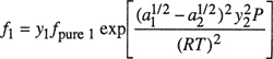
Figure 3-2 presents fugacity coefficients for several hydrocarbons in binary mixtures with nitrogen. In these calculations, Eq. (3-34) was used with y₁ = 0.10 and T = 343 K; in each case, component 2 is nitrogen. For comparison, we also show the fugacity coefficient of butane according to the Lewis fugacity rule; in that calculation, the second exponential in Eq. (3-34) was neglected. From Eq. (3-36) we see that the Lewis rule is poor for butane for two reasons: First, the mole fraction of butane is small (hence near unity), and second, the difference in intermolecular forces between butane and nitrogen (as measured by is large. If the gas in excess were hydrogen or helium instead of nitrogen, the deviations from the Lewis rule for butane would be even larger.

Figure 3-2 Fugacity coefficients of light hydrocarbons in binary mixtures with nitrogen at 343 K. Calculations based on simplified form of van der Waals’ equation.

For a component i, the Lewis fugacity rule is often poor when y_i<<1. However, the Lewis fugacity rule is usually good when y_i is close to unity because it becomes exact when y_i = 1.

3.3 Fugacity of a Pure Liquid or Solid

The derivation of Eq. (3-16) is general and not limited to the vapor phase. It may be used to calculate the fugacity of a pure liquid or that of a pure solid. Such fugacities are of importance in phase-equilibrium thermodynamics because we frequently use a pure condensed phase as the standard state for activity coefficients.

To calculate the fugacity of a pure solid or liquid at given temperature T and pressure P, we separate the integral in Eq. (3-16) into two parts: The first part gives the fugacity of the saturated vapor at T and P^s (the saturation pressure), and the second part gives the correction due to the compression of the condensed phase to pressure P. At saturation pressure P^s, the fugacity of saturated vapor is equal to the fugacity of the saturated liquid (or solid) because the saturated phases are in equilibrium. Let superscript s refer to saturation and superscript c refer to condensed phase. Equation (3-16) for a pure component is now rewritten

(3-37)

The first term on the right-hand side gives the fugacity of the saturated vapor, equal to that of the saturated condensed phase. Equation (3-37) becomes

(3-38)

that can be rearranged to yield

(3-39)

where

Equation (3-39) gives the important result that the fugacity of a pure condensed component i at T and P is, to a first approximation, equal to , the saturation (vapor) pressure at T. Two corrections must be applied. First, the fugacity coefficient corrects for deviations of the saturated vapor from ideal-gas behavior. Second, the exponential correction (often called the Poynting correction) takes into account that the liquid (or solid) is at a pressure P different from . In general, the volume of a liquid (or solid) is a function of both temperature and pressure, but at conditions remote from critical, a condensed phase may often be regarded as incompressible and in that case the Poynting correction takes the simple form

The two corrections are often, but not always, small and sometimes they are negligible. If temperature T is such that the saturation pressure is low (say below 1 bar), then is very close to unity.³

³ There are, however, a few exceptions. Substances that have a strong tendency to polymerize (e.g., acetic acid or hydrogen fluoride) may show significant deviations from ideal-gas behavior even at pressures near or below 1 bar. see Sec. 5.9.

Figure 3-3 gives fugacity coefficients for four liquids at saturation; these coefficients were calculated with Eq. (3-37) using vapor-phase volumetric data. Because the liquids are at saturation conditions, no Poynting correction is required.

Figure 3-3 Fugacity coefficients from vapor-phase volumetric data for four saturated liquids.

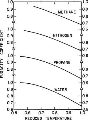
We see that when plotted against reduced temperature, the results for the four liquids are almost (but not quite) superimposable; further, we note that differs considerably from unity as the critical temperature is approached. The correction always tends to decrease the fugacity because for all pure, saturated substances < 1.

The Poynting correction is an exponential function of the pressure; it is small at low pressure but may become large at high pressures or at low temperatures. To illustrate, Table 3-1 gives some numerical values of the Poynting correction for an incompressible component with = 100cm³mol^-1 and T- 300 K.

Table 3-1 The Poynting correction: effect of pressure on fugacity of a pure, condensed and incompressible substance whose molar volume is 100 cm³ mol^-1 (T= 300 K).

Figure 3-4 shows the fugacity of compressed liquid water as a function of pressure for three temperatures; the fugacities were calculated from thermodynamic properties reported by Keenan et al. (1978). The lowest temperature is much less, whereas the highest temperature is just slightly less than the critical temperature, 374°C. The saturation pressures are also indicated in Fig. 3-4. We see that, as indicated by Eq. (3-39), the fugacity of compressed liquid water is more nearly equal to the saturation pressure than to the total pressure. At the highest temperature, liquid water is no longer incompressible and its compressibility cannot be neglected in the Poynting correction.

Figure 3-4 Fugacity of liquid water at three temperatures from saturation pressure to 414 bar. The critical temperature of water is 374°C.

3.4 Thermodynamic Properties with Independent Variables V and T

In Sec. 3.1 we gave expressions for the thermodynamic properties in terms of independent variables P and T. Because volumetric properties of fluids are usually (and more simply) expressed by equations of state that are pressure-explicit,⁴ it is more convenient to calculate thermodynamic properties in terms of independent variables V and T.

⁴ If the equation of state is to hold for both vapor and liquid phases, it must necessarily be pressure-explicit. For example, water at 100°C and 1 atm has two equilibrium phases with much different volumes: saturated steam and liquid water. At a fixed P and T, a volume-explicit equation gives only one value for V. But a pressure-explicit equation, at fixed P and T, can give two or more values for V.

At constant temperature and composition, we use one of Maxwell’s relations to give the effect of volume on energy and entropy:

(3-40)

(3-41)

These two equations form the basis of the derivation for the desired equations. Again, we do not present the derivation but refer to the publications of Beattie.

First, expressions are found for the energy and entropy. The other properties are then calculated from their definitions:

(3-42)

(3-43)

(3-44)

(3-45)

(3-46)

The results are given in Eqs. (3-47) to (3-53). As in Sec. 3.1, it is understood that all integrations are performed at constant temperature and composition. The symbols are the same as those defined after Eq. (3-7) with one addition:

molar energy of pure i as an ideal gas at temperature T.

In Eqs. (3-49) to (3-52), the units of V/n_iRN are bar^-1. Because the independent variable in Eqs. (3-47) to (3-49) is the volume, no additional terms for change of phase (e.g., enthalpy of vaporization) need be added to these equations when they are applied to a condensed phase.

(3-47)

(3-48)

(3-49)

(3-50)

(3-51)

(3-52)

and finally,

(3-53)

where z = Pv/RT Is the compressibility factor of the mixture.

Equation (3-53) gives the fugacity of component i in terms of independent variables V and T; it is similar to Eq. (3-14) that gives the fugacity in terms of independent variables P and T. However, in addition to the difference in the choice of independent variables, there is another, less obvious difference: Whereas in Eq. (3-14) the key term is , the partial molar volume of i, in Eq. (3-53) the key term is and that is not a partial molar quantity.⁵

⁵ The definition of a partial molar property is applicable only to extensive properties differentiated at constant temperature and pressure. The total volume of a mixture is related to the partial molar volumes by a summation: . The analogous equation for the total pressure is not valid: . The derivative should not be regarded as a partial pressure; it does not have a significance analogous to that of the partial molar volume.

For a pare component Eq. (3-53) becomes

(3-54)

Equation (3-54) is not particularly useful; for a pure component, Eq. (3-17) is much more convenient. However, for mixtures, Eq. (3-53) is more useful than Eq. (3-14).

Equations (3-47) to (3-53) enable us to compute all thermodynamic properties relative to the properties of an ideal gas at 1 bar and at the same temperature and composition, provided that we have information on volumetric behavior in the form

(3-55)

Most equations of state are pressure-explicit [Eq. (3-55)] rather than volume-explicit [Eq. (3-15)]. Therefore, for phase-equilibrium problems, Eq. (3-53) is more useful than Eq. (3-14).

To use Eq. (3-53) for calculating the fugacity of a component in a mixture, volumetric data must be available, preferably in the form of an equation of state, at the temperature under consideration and as a function of composition and density, from zero density to the density of interest that corresponds to the lower limit V in the integral. The molar density of the mixture, n_T / V, corresponding to the lower integration limit, must often be found from the equation of state itself; because the specified conditions are usually composition, temperature, and pressure, the density is not ordinarily given. This calculation is tedious because it is usually of the trial-and-error type. However, regardless of the number of components in the mixture, the calculation need only be performed once for any given composition, temperature, and pressure; because the quantity V in Eq. (3-53) is for the entire mixture, it can be used in the calculation of the fugacities for all components. Only if the composition, temperature, or pressure changes must the trial-and-error calculation be repeated. It is probably because of the need for trial-and-error calculations that many authors of classic books on thermodynamics have paid little attention to Eq. (3-53). While trial-and-error calculations were highly undesirable before about 1960, in the age of computers they cause little concern.

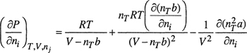
For some applications like those requiring derived properties (e.g. composition derivatives of fugacity coefficients), one can achieve considerable computational simplification (Topliss et al., 1988; Mollerup and Michelsen, 1992) in the calculation of thermodynamic properties when relations for the desired properties are defined in terms of (ρ, T, x_i) instead of (V, T, n_i), as in the equations above. Here, ρ is the molar density corresponding to pressure P, temperature T, and composition of the phase of interest, and x_i = n_i/n_T is the mole fraction of component i.

For a given equation of state, the associated expression for the compressibility factor is

(3-56)

The reduced molar residual Helmholtz energy, Ã = A^r/n_TRT, is given by

(3-57)

The adjective “residual” means that the quantity is defined relative to a mixture of ideal gases at the same density, temperature, and composition as those of the mixture of interest.

The associated expression for the fugacity coefficient of component i becomes

(3-58)

For a mixture with m components, the derivative of à with respect to the number of moles of component i is

(3-59)

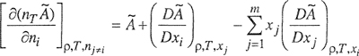
where the differential operator (D/Dx_i) x_i indicates differentiation with respect to x_i while all other x_j are held constant.

Similarly, we can derive equations of the partial derivatives of Inφ_i with respect to pressure (at constant temperature and composition), with respect to temperature (at constant pressure and composition), and with respect to composition (at constant pressure and temperature). Therefore, these equations relate the desired thermodynamic properties to à and derivatives of à with respect to its independent variables.

The main advantage of Eqs. (3-58) and (3-59) is that the fugacities are obtained from à by differentiation [Eq. (3-58)] rather than by integration of terms obtained from the equation of state [Eq. (3-53)]. It is easier to differentiate than to integrate and not every expression is analytically integrable. To use Eqs. (3-58) and (3-59) it is necessary to have a model for à as a function of temperature, density, and composition.

Topliss (1988) and Dimitrelis (1986) give efficient computation methods for phase equilibria using this formalism.

3.5 Fugacity of a Component in a Mixture According to van der Waals’ Equation

To illustrate the applicability of Eq. (3-53), we consider a mixture whose volumetric properties are described by van der Waals’ equation:

(3-60)

In Eq. (3-60), υ is the molar volume of the mixture and a and b are constants that depend on composition.

To substitute Eq. (3-60) into Eq. (3-53), we must first transform it from a molar basis to a total basis by substituting υ = V/n_T, where n_T is the total number of moles. Equation (3-60) then becomes

(3-61)

We want to calculate the fugacity of component i in the mixture at some given temperature, pressure, and composition. Differentiating Eq. (3-61) with respect to n_i, we have

(3-62)

Substituting into Eq. (3-53) and integrating, we obtain

(3-63)

At the upper limit of integration, as V → ∞,

(3-64)

and Eq. (3-63) becomes

(3-65)

Equation (3-65) gives the desired result derived from rigorous thermodynamic relations. To proceed further, it is necessary to make assumptions concerning the composition dependence of constants a and b. These assumptions cannot be based on thermodynamic arguments but must be obtained from molecular considerations. Suppose that we have m components in the mixture. If we interpret constant b as a term proportional to the size of the molecules and if we assume that the molecules are spherical, then we might average the molecular diameters, giving

(3-66)

On the other hand, we may choose to average the molecular volumes directly and obtain the simpler relation

(3-67)

Neither Eq. (3-66) nor Eq. (3-67) is in any sense a “correct” mixing rule; both are based on arbitrary assumptions, and alternative mixing rules could easily be constructed based on different assumptions. Equation (3-67) is commonly used because of its mathematical simplicity.

At moderate densities, for mixtures whose molecules are not too dissimilar in size, the particular mixing rule used for b does not significantly affect the results. However, the fugacity of a component in a mixture is sensitive to the mixing rule used for the constant a. If we interpret a as a term that reflects the strength of attraction between two molecules, then for a mixture we may want to express a by averaging over all molecular pairs. Thus

(3-68)

where a_ij is a measure of the strength of attraction between a molecule i and a molecule j. If i and j are the same chemical species, then a_ij is the van der Waals a for that substance. If i and j are chemically not identical and if we have no experimental data for the i-j mixture, we then need to express a_ij in terms of a_i and a_j. This need constitutes one of the key problems of phase-equilibrium thermodynamics. Given information on the intermolecular forces of each of two pure fluids, how can we predict the intermolecular forces in a mixture of these two fluids? There is no general answer to this question. An introduction to the study of intermolecular forces is given in Chap. 4 where it is shown that only under severe limiting conditions can the forces between molecule i and molecule j be related in a simple way to the forces between two molecules i and two molecules j. Our knowledge of molecular physics is, unfortunately, not sufficient to give generally reliable methods for predicting the properties of mixtures using only knowledge of the properties of pure components.

For i ≠ j, it was suggested many years ago by Berthelot, on strictly empirical grounds, that

(3-69)

This relation, often called the geometric-mean assumption, was used extensively by van der Waals and his followers in their work on mixtures. Since van der Waals’ time, the geometric-mean assumption has been used for other quantities in addition to van der Waals’ a; it is commonly used for those parameters that are a measure of intermolecular attraction. Long after the time of van der Waals and Berthelot, it was shown by London (see Sec. 4.4) that under certain conditions there is some theoretical justification for the geometric-mean assumption.

If we adopt the mixing rules given by Eqs. (3-67), (3-68), and (3-69), the fugacity for component i, given by Eq. (3-65), becomes

(3-70)

where υ is the molar volume and z is the compressibility factor of the mixture.

Equation (3-70) indicates that, to calculate the fugacity of a component in a mixture at a given temperature, pressure, and composition, we must first compute constants a and b for the mixture using some mixing rules, for example, those given by Eqs. (3-67), (3-68), and (3-69). Using these constants and the equation of state, Eq. (3-60), we must then find the molar volume υ of the mixture by Cardan’s method or by trial and error; this step is the only tedious part of the calculation. Once the molar volume is known, the compressibility factor z is easily calculated and the fugacity is readily found from Eq. (3-70).

For a numerical example, consider the fugacity of hydrogen in a ternary mixture at 50°C and 303 bar containing 20 mol % hydrogen, 50 mol % methane, and 30 mol % ethane. Using Eq. (3-70), we find that the fugacity of hydrogen is 114.5 bar.⁶ From the ideal-gas law, the fugacity is 60.8 bar, while the Lewis fugacity rule gives 72.3 bar. These three results are significantly different from one another. No reliable experimental data are available for this mixture at 50°C but in this particular case it is probable that 114.5 bar is much closer to the correct value than the results of either of the two simpler calculations. However, such a conclusion cannot be generalized. The equation of van der Waals gives only an approximate description of gas-phase properties and sometimes, because of cancellation of errors, calculations based on simpler assumptions may give better results.

⁶ Constants a and b for each component were found from critical properties. The molar volume of the mixture, as calculated from van der Waals’ equation, is 62.43 cm³ mol¹.

In deriving Eq. (3-70) we have shown how the rigorous expression, Eq. (3-53), can be used to calculate the fugacity of a component in a mixture once the equation of state for the mixture is given. In this particular calculation, the relatively simple van der Waals equation was used but the same procedure can be applied to any pressure-explicit equation of state, regardless of how complex it may be.

It is frequently said that the more complicated an equation of state, and the more constants it contains, the better representation it gives of volumetric properties. This statement is correct for a pure component if ample data are available to determine the constants with confidence and if the equation is used only under those conditions of temperature and pressure used to determine the constants. However, for predicting the properties of mixtures from pure-component data alone, the more constants one has, the more mixing rules are required and, because these rules are subject to much uncertainty, it frequently happens that a simple equation of state containing only two or three constants is better for predicting mixture properties than a complicated equation of state containing a large number of constants (Ackerman and Redlich, 1963; Shah and Thodos, 1965).

Chapter 5 discusses the use of equations of state for calculating fugacities in gas-phase mixtures and Chap. 12 discusses such use for calculating fugacities in both gas-phase and liquid-phase mixtures.

3.6 Phase Equilibria from Volumetric Properties

In Chap. 1 we indicated that the purpose of phase-equilibrium thermodynamics is to predict conditions (temperature, pressure, composition) which prevail when two or more phases are in equilibrium.

In Chap. 2 we discussed thermodynamic equations that determine the state of equilibrium between phases α and β. These are:⁷

⁷ Note, however, the restrictions indicated in the footnote at the beginning of Sec. 2.3.

Equality of temperatures:	Tα = Tβ
Equality of pressures:	Pα = Pβ
For each component i, equality of fugacities:	fiα = fiβ

To find the conditions that satisfy these equations, it is necessary to have a method for evaluating the fugacity of each component in phase α and in phase β. Such a method is supplied by Eq. (3-14) or (3-53); both are valid for any component in any phase. In principle, therefore, a solution to the phase-equilibrium problem is provided completely by either one of these equations together with an equation of state and the equations of phase equilibrium.

To illustrate these ideas, consider vapor-liquid equilibria⁸ in a system with m components; suppose that we know pressure P and mole fractions x₁, x₂,…,x_m, for the liquid phase. We want to find temperature T and vapor-phase mole fractions y₁, y₂,…, y_m. We assume that we have available a pressure-explicit equation of state applicable to all components and to their mixtures over the entire density range, from zero density to the density of the liquid phase.

⁸ Because the equations relating chemical potential (or fugacity) to volumetric properties use integrals starting from zero density, evaluation of these integrals requires continuity from zero density to the density of interest. While it is possible to go continuously from vapor to liquid, it is not possible to go continuously from either fluid to a crystalline solid. Therefore, the discussion here is not applicable to fluid-solid equilibria.

We can then compute the fugacity of each component, in either phase, by Eq. (3-53).

The number of unknowns is:

⁹ Because Σ_i y_i = 1, the mth mole fraction is fixed once (m - 1) mole fractions are determined.

The number of independent equations is:

Because the number of unknowns is equal to the number of independent equations, the unknown quantities can be found by simultaneous solution of all equations.¹⁰ It is apparent, however, that the computational effort to do so is large, especially if the equation of state is not simple and if the number of components is high.

¹⁰ We have considered here the case where P and x are known and T and y are unknown, but similar reasoning applies to other combinations of known and unknown quantities; the number of intensive variables that must be specified is given by the phase rule.

Calculation of vapor-liquid equilibria, along the lines outlined, was discussed many years ago by van der Waals who made use of the equation bearing his name, and in the period 1940-1952 extensive calculations for hydrocarbon mixtures were reported by Benedict et al. (1940, 1942, 1951) who used an eight-constant equation of state. Since that pioneering work, many others have made similar calculations using a variety of equations of state, as discussed in Chap. 12.

Calculation of phase equilibria from volumetric data alone requires a large computational effort but, thanks to modern computers, the effort does not by itself present a significant difficulty. The major disadvantage of this type of calculation is not computational; the more fundamental difficulty is that we do not have a satisfactory equation of state applicable to mixtures over a density range from zero density to liquid densities. Because of this crucial deficiency, phase-equilibrium calculations based on volumetric data alone are often doubtful. To determine the required volumetric data with the necessary degree of accuracy, a large amount of experimental work is required; rather than make all these volumetric measurements, it is usually more economical to measure the desired phase equilibria directly. For those mixtures where the components are chemically similar (e.g., mixtures of paraffinic and olefinic hydrocarbons) an equation-of-state calculation for vapor-liquid equilibria provides a reasonable possibility because many simplifying assumptions can be made concerning the effect of composition on volumetric behavior. But even in this relatively simple situation, there is much ambiguity when one attempts to predict properties of mixtures using equation-of-state constants determined from pure-component data. Benedict et al. used eight empirical constants to describe the volumetric behavior of each pure hydrocarbon; to fix uniquely eight constants, a very large amount of experimental data is required. Even with the generous amount of data that Benedict had at his disposal, his constants could not be determined without some ambiguity. But the essence of the difficulty arises when one must decide on mixing rules, i.e., on how these constants are to be combined for a mixture. Phase-equilibrium calculations are often sensitive to the mixing rules used, especially to the binary parameters that appear in these rules.

In summary, then, the equation-of-state method to attain a complete determination of phase equilibria is often not promising because we usually do not have sufficiently accurate knowledge of the volumetric properties of mixtures at high densities. Calculation of fugacities by Eq. (3-53) is practical for vapor mixtures but, special cases excepted, may not be practical for condensed mixtures. Even in vapor mixtures, the calculations are often not accurate because of our inadequate knowledge of volumetric properties. The accuracy of the fugacity calculated with Eq. (3-53) depends directly on the validity of the equation of state and, to determine the constants in a good equation of state, one must have either a large amount of reliable experimental data, or else some sound theoretical basis for predicting volumetric properties. For many mixtures we have little of either data or theory. Reliable volumetric data exist for the more common substances but these constitute only a small fraction of the number of listings in a chemical handbook. Reliable volumetric data are scarce for binary mixtures and they are rare for mixtures containing more than two components. Considering the nearly infinite number of ternary (and higher) mixtures possible, it is clear that there will never be sufficient experimental data to give an adequate empirical description of volumetric properties of mixed fluids. A strictly empirical approach to the phase equilibrium problem is, therefore, subject to severe limitations. Progress can be achieved only by generalizing from limited, but reliable, experimental results, utilizing as much as possible techniques based on our theoretical knowledge of molecular behavior. Since the first edition of this book (1969) remarkable progress has been made; based on statistical mechanical derivations, promising equations of state are now available, for example, for polar and for hydrogen-bonded fluids, for electrolytes and colloidal particles in water, and for polymeric systems. Many of these advanced equations of state are beyond the scope of this book.

Significant progress in phase-equilibrium thermodynamics can be achieved only by increased use of the concepts of molecular physics. Therefore, before continuing our discussion of fugacities in Chap. 5, we turn in Chap. 4 to a brief survey of intermolecular forces.

References

Ackerman, F, J. and O. Redlich, 1963, J. Chem. Phys., 38: 2740.

Beattie, J. A. and W. H. Stockmayer, 1942. In Treatise on Physical Chemistry, (H. S. Taylor and S. Glasstone, Eds.), Chap. 2. Princeton: Van Nostrand.

Beattie, J. A., 1949, Chem. Rev., 44: 141.

Beattie, J. A., 1955. In Thermodynamics and Physics of Matter, (F. D. Rossini, Ed.), Chap. 3, Part C. Princeton: Princeton University Press.

Benedict, M., G. B. Webb, and L. C. Rubin, 1940, J. Chem. Phys., 8: 334.

Benedict, M., G. B. Webb, and L. C. Rubin, 1942, J. Chem. Phys., 10: 747.

Benedict, M., G. B. Webb, and L. C. Rubin, 1951, Chem. Eng. Prog., 47: 419.

Dimitrelis, D. and J. M. Prausnitz, 1986, Fluid Phase Equilibria, 31: 1.

Evans, R. B. and G. M. Watson, 1956, Chem. Eng. Data Series, 1: 67.

Keenan, J. H., F. G. Keyes, P. G. Hill, and J. G. Moore, 1978, Steam Tables: Thermodynamic Properties of Water Including Vapor, Liquid and Solid Phases. New York: WiSey-Interscience.

Mollerup, J. M. and M. L. Michelsen, 1992, Fluid Phase Equilibria, 74: 1.

Shah, K. K. and G. Thodos, 1965, Ind. Eng. Chem., 57: 30.

Topliss, R. J., D. Dimitrelis, and J. M. Prausnitz, 1988, Comput. Chem. Engng., 12: 483.

Problems

1. Consider a mixture of m gases and assume that the Lewis fugacity rule is valid for this mixture. For this case, show that the fugacity of the mixture f_mixt is given by where y_i is the mole fraction of component i and f_{pure i} is the fugacity of pure component i at the temperature and total pressure of the mixture.

2. A binary gas mixture contains 25 mol % A and 75 mol % B. At 50 bar total pressure and 100°C the fugacity coefficients of A and B in this mixture are, respectively, 0.65 and 0.90. What is the fugacity of the gaseous mixture?

3. At 25°C and 1 bar partial pressure, the solubility of ethane in water is very small; the equilibrium mole fraction is x_C2H6 = 0.33 × 10^-4. What is the solubility of ethane at 25°C when the partial pressure is 35 bar? At 25°C, the compressibility factor of ethane is given by the empirical relation

z = 1 -7.63 × 10^-3P – 7.22x10^-5P²

where P is in bar. At 25°C, the saturation pressure of ethane is 42.07 bar and that of water is 0.0316 bar.

4. Consider a binary mixture of components 1 and 2. The molar Helmholtz energy change Δa is given by

where υ is the molar volume of the mixture; b is a constant for the mixture, depending only on composition; and Δa is the molar Helmholtz energy change in going isothermally from the standard state (pure, unmixed, ideal gases at 1 bar) to the molar volume υ. The composition dependence of b is given by b =y₁y_b + y₂b₂ Find an expression for the fugacity of component 1 in the mixture.

5. Derive Eq. (3-54). [Hint: Start with Eq. (3-51) or with Eq. (3-53).]

6. Oil reservoirs below ground frequently are in contact with underground water and, in connection with an oil drilling operation, you are asked to compute the solubility of water in a heavy oil at the underground conditions. These conditions are estimated to be 140°C and 410 bar. Experiments at 140°C and 1 bar indicate that the solubility of steam in the oil is x₁ = 35 x 10^-4 (x₁ is the mole fraction of steam). Assume Henry’s law in the form f₁ = H(T) x₁ where H(T) is a constant, dependent only on the temperature, and f₁ is the fugacity of H₂O. Also assume that the vapor pressure of the oil is negligible at 140°C. Data for H2O are given in the steam tables.

7. A gaseous mixture contains 50 mol % A and 50 mol % B. To separate the mixture, it is proposed to cool it sufficiently to condense the mixture; the condensed liquid mixture is then sent to a distillation column operating at 1 bar. Initial cooling to 200 K (without condensation) is to be achieved by Joule-Thomson throttling. If the temperature upstream of the throttling valve is 300 K, what is the required upstream pressure? The volumetric properties of this gaseous mixture are given by

where υ is the volume per mole of mixture in cm³ mol^-1. The ideal-gas specific heats are:

8. Some experimental data for the region from 0 to 50 bar indicate that the fugacity of a pure gas is given by the empirical relation

where P is the pressure (bar) and c and d are constants that depend only on temperature. For the region 60 to 100°C, the data indicate that

where T is in kelvin. At 80°C and 30 bar, what is the molar enthalpy of the gas relative to that of the ideal gas at the same temperature?

9. A certain cryogenic process is concerned with an equimolar mixture of argon (1) and ethane (2) at 110 K. To design a separation process, a rough estimate is required for the enthalpy of mixing for this liquid mixture. Make this estimate using van der Waals’ equation of state with the customary mixing rules, and with . Assume that and because pressure is low, that where U is the internal energy and H is the enthalpy. Data are:

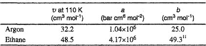
¹¹ This b is obtained from critical volume. The inadequacy of the van der Waals equation is evident because, as shown here, b > υ at 110 K. Fortunately this unrealistic result does not affect the solution to Problem 9.

Second-virial-coefficient data for this mixture indicate that k_ij (i ≠ j) = 0.1.