Appendix H
Brief Introduction to Perturbation Theory of Dense Fluids

Statistical mechanics provides a powerful tool for representing the equilibrium properties of pure and mixed fluids because it provides the link between microscopic and macroscopic properties; if we can establish some quantitative relations concerning the properties of a small assembly of molecules, statistical mechanics provides a method for “scaling up” those relations to apply to a very large number of molecules. These scale-up relations can then be compared with ordinary therrnodynamic properties as measured in typical (macroscopic) experiments.

Because we do not have a satisfactory physical understanding of dense fluids, we cannot establish a truly satisfactory theory of dense fluids (except for very simple cases). This difficulty does not follow from inadequate statistical mechanics but from inadequate knowledge of fluid structure and intermolecular forces. To overcome this difficulty, it has become common practice, first, to focus attention on the properties of some idealized dense fluid, and second, to relate the properties of a real dense fluid to those of the idealized fluid. This procedure is the essence of perturbation theory.

The philosophical basis of perturbation theory is very old; the fundamental ideas can be found in ancient Greek texts (e.g., Plato) and they have had a profound influence on science: Because the properties of nature are not easily understood, it is useful to postulate an idealized nature (whose properties can be specified) and then to establish “corrections” that take into account differences between real and idealized nature. In this context, the words “correction” and “perturbation” are equivalent. If we choose a good idealization, the “corrections” will be small; in that event, first-order perturbations will be sufficient.

In statistical thermodynamics, the best-known perturbation theory is the virial equation for imperfect gases at modest densities. The reference system (idealized fluid) is the ideal gas; compressibility factor z is written as an expansion in density p about Z₀, where subscript 0 stands for the reference system.

For a fluid at constant temperature and composition,

where

(H-1)

where

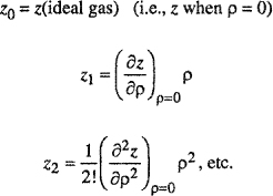
As discussed in Chap. 5, the first perturbation term (z₁) leads to the second virial coefficient, the second perturbation term leads to the third virial coefficient, and so on. Because the reference system is an ideal gas, Eq. (H-l) is useful only for gases not excessively far from the ideal-gas state. The two most important requirements for a good perturbation theory are that the reference system is as close as possible to the real system and that the properties of the reference system are known accurately.

For dense fluids, it is clear that an ideal gas would be a very bad reference system. To describe dense fluids well, the key problem is to choose a suitable (idealized) reference fluid. Much attention has been given to this problem, as discussed in numerous references. Here we give only a short introduction to indicate some basic ideas.

Consider N molecules of a pure fluid at volume V and temperature T. As discussed in any book on statistical mechanics and as briefly reviewed in App. B, the Helmholtz energy A can be divided into two contributions: The first depends only on temperature, while the second depends also on density. It is only the second part,called the configurational Helmholtz energy that is of interest here, because only configurational properties depend on intermolecular forces.

Consistent with the purposes of this introduction, we now limit attention to fluids containing small spherical molecules.¹ The configurational Helmholtz energy of a classical fluid² is written³

(H-2)

where U is the total potential energy of the fluid and r₃ is the position of molecule 1, etc.

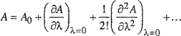
We want to expand A as a power series in some perturbing parameter λ such that at constant temperature and density,

(H-3)

where subscript 0 refers to the reference system and where

(H-4)

(H-5)

The perturbation parameter λ is defined through potential energy U,

(H-6)

where subscript p stands for perturbation. Here U_o is the (total) reference potential and U_p is the total perturbation potential such that when λ= 1, U_λ is the total potential of the real fluid.

When λ= 1, we obtain the desired perturbation expansion,

(H-7)

¹ Ingeneral, perturbation methods are not limited to small spherical molecules; in principle they are applicable to fluids containing molecules of arbitrary complexity.

² A classical fluid is one whose properties are described by classical (as opposed to quantum) mechanics.

³ To simplify notation, we use only a single integral sign to denote multiple integration over all coordinates.

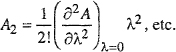
To obtain the first-order perturbation, we first write

(H-8)

where

(H-9)

Differentiating with respect to λ yields

(H-10)

Because ∂Uλ∂λ =U_p Eq. (H-10) can be rewritten

(H-11)

where < > designates an ensemble average:

(H-12)

To find A_t, we set λ= 0 because

(H-13)

Equation (H-13) says that the first-order perturbation term A j can be found by calculating an ensemble average of the perturbation energy U_p where the ensemble average is calculated using properties (U₀ and Z₀) of the reference system. To illustrate this important feature of perturbation theory, consider the case where the total perturbation energy is assumed to be the sum of all pair perturbation energies:

(H-14)

where r_ij is the center-to-center distance between any two molecules i and j. The pair perturbation potential, r_ij is defined in a manner analogous to Eq. (H-6). For any pair of molecules.

(H-15)Γ

When λ= 1,Γ_λ is the pair potential of the real system. It can then be shown (Smith, 1973) that

(H-16)

where p is the number density, p = N/V, and where r is the center-to-center distance between any arbitrary molecule and some other arbitrary fixed molecule whose center is chosen to be the origin of the coordinate system.

To understand the physical meaning of A₁ let us first ignore g0(r), the radial distribution function of the reference system. Imagine a sphere of radius r whose center is the center of an arbitrarily chosen fixed molecule. The area of that sphere is 4 πr ². Now imagine a thin shell of height dr built on that sphere’s surface; the volume of that shell is 4πr₂dr. The number of molecular centers in that shell is the volume of the shell multiplied by p.

Focusing on the molecule at the center, Γ_p(r) is the perturbation contribution of any one molecule at some distance r. The integral gives the contributions of all molecules, at all distances r. The factor 2 (instead of 4) arises in Eq. (H-16) because Γ_p(r) is the perturbation potential for two molecules.

Because molecules have a nonzero size, the number of molecular centers in the shell at distance r is not necessarily Np. For example, suppose r is very small, smaller than molecular diameter CT. In that event, the number of molecular centers in the shell is not Np but zero. For an assembly of molecules whose diameters are σ, where σ >0 the number of molecular centers in a shell at distance r must depend on the dimensioaless distance r/σ

Given that a molecular center is at r = 0, we must ask: What is the number of molecular centers in a shell of thickness dr at position r? This number is related to the radial distribution function g(r):

Number of molecular centers between r and r + dr

Radial distribution function g(r) gives information on the microscopic structure of an assembly of molecules.⁴ For a structureless fluid (e.g., ideal gas), g(r) - 1 and for a lattice g(r) is a periodic function. For real fluids (σ> 0), g(r) is zero at small r, rises to above unity in the vicinity where r is just slightly larger than σ(shell of first neighbors), and then oscillates about unity, asymptotically approaching unity as r >> σ, as illustrated in Fig. H-l.

⁴ More property, for a pare fluid g(r) it should be written g(r, p, T) because it depends not only on r, but also on density p and temperature T. For a mixture, it should be written g(r, p, T, x) because it also depends on composition x.

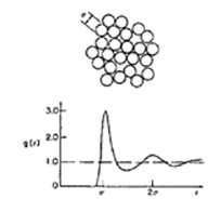
The important feature of Eq. (H-16) is that the radial distribution function in the integral, g₀(r), is not that of the real system, that is not known, but that of the reference system, that is known. This follows directly from Eq. (H-12), where the averaging procedure to find <U_p> is based on properties of the reference system.

Figure H-1 Radial distribution function for a simple dense fluid.

Although this discussion has been limited to pure fluids containing spherical molecules, the same ideas can be applied to pure or mixed fluids containing complex molecules, as discussed elsewhere (Reed and Gubbins, 1973; Gray and Gubbins, 1984; Lucas, 1991). Further, while the discussion here has been limited to first-order perturbation theory, it is possible to construct perturbation theories for second, third, and higher orders. However, when we consider nonspherical molecules and when we consider second-order (or higher) perturbations, not only does mathematical complexity rise but also much more detailed information on fluid structure and intermolecular forces is required.

It is likely that perturbation theories will become increasingly useful in phaseequilibrium thermodynamics. However, when applied to mixtures of real fluids, calculations are not only long but also nonanalytic; numerical integrations are required for every temperature, density, and composition. Further, when applied to real mixtures, considerable ingenuity is required to establish a useful reference system, and intermolecular forces must be characterized through credible potential functions. With increasingly efficient computers and with advances in molecular physics, perturbation theory of fluids is likely to provide an increasingly powerful tool for molecular thermodynamics.

References

Chandler, D., 1987, Introduction to Modem Statistical Mechanics. New York: Oxford University Press.

Gray, C. G. and K. E. Gubbins, 1984, Theory of Molecular Fluids. Oxford: Clarendon Press.

Lucas, K., 1991, Applied Statistical Thermodynamics. Berlin: Springer.

McQuarrie, D. A., 1976, Statistical Mechanics. New York: Harper & Row.

McQuarrie, D. A., 1985, Statistical Thermodynamics. Mill Valley: University Science Books.

Reed, T. M. and K. E. Gubbins, 1973, Applied Statistical Mechanics. New York: McGraw-Hill (Reprinted by Butterworth-Heinemann, 1991).

Smith, W. R., 1973. In Statistical Mechanics, (K. Singer, Ed.), Specialist Periodical Report. London: The Royal Society of Chemistry.